Flow-Level Performance and Capacity
of Wireless Networks with User Mobility
Thomas Bonald∗, Sem Borst†,?, Nidhi Hegde∗, Matthieu Jonckheere?, Alexandre Proutiere‡ ∗Orange Labs, Paris, France
†Bell Labs, Alcatel-Lucent, P.O. Box 636, Murray Hill, NJ 07974, USA
?Department of Mathematics & Computer Science, Eindhoven University of Technology P.O. Box 513, 5600 MB Eindhoven, The Netherlands
‡Microsoft Research, Cambridge, England September 6, 2009
Abstract
The performance evaluation of wireless networks is severely complicated by the specific features of radio communication, such as highly variable channel conditions, interference issues, and possible hand-offs among base stations. The latter elements have no natural counterparts in wireline scenarios, and create a need for novel performance models that account for the impact of these characteristics on the service rates of users.
Motivated by the above issues, we review several models for characterizing the capacity and evaluating the flow-level performance of wireless networks carrying elastic data transfers. We first examine the flow-level performance and stability of a wide family of so-calledα-fair channel-aware scheduling strategies. We establish that these disciplines provide maximum stability, and describe how the special case of the Proportional Fair policy gives rise to a Processor-Sharing model with a state-dependent service rate. Next we turn attention to a network of several base stations with inter-cell interference. We derive both necessary and sufficient stability conditions and construct lower and upper bounds for the flow-level per-formance measures. Lastly we investigate the impact of user mobility that occurs on a slow time scale and causes possible hand-offs of active sessions. We show that the mobility tends to increase the capacity region, both in the case of globally optimal scheduling and local α-fair scheduling. It is additionally demonstrated that the capacity and user throughput improve with lower values of the fairness indexα.
1
Introduction
The performance evaluation of wireless networks centers on similar metrics as in wireline envi-ronments, such as user-perceived throughputs, delay characteristics, and loss rates. However, the evaluation of these performance metrics is severely complicated by the specific features of wireless communications, e.g., uncertain and highly variable channel conditions, interfer-ence issues, and possible hand-offs among base stations (BS’s) associated with long-range user mobility. The latter features have no natural counterparts in wireline scenarios, and create a strong need to develop and analyze novel models for the performance evaluation of wireless networks. In fact, even the characterization of the network capacity, which is straightforward in
wireline systems with fixed link rates, becomes non-trivial in the presence of channel variations, and even mostly intractable in the case of mutual interference.
In order to develop adequate performance models for wireless networks, it is crucial to identify the primary sources of channel variations. First of all, the channel quality may differ widely among spatially distributed users due to distance-related attenuation. In addition, the channel conditions for a given user may vary dramatically over time because of fading effects. Fading is an extremely complex physical phenomenon caused by the interaction between the propagation environment and user mobility. It emerges in diverse forms and typically spans a wide range of time scales. Multi-path fading arises on the level of a wavelength, and occurs on a fast time scale that depends on the carrier frequency and user velocity. Path loss and shadow fading manifest themselves on a more macroscopic level as a result of distance-related attenuation and scattering due to obstacles and terrain conditions, and tend to vary over a longer time scale. Variations in the path loss due to long-range user mobility force hand-offs of active sessions, and cause a dynamic interaction among neighboring BS’s. As a further potential source of complex interaction, transmissions tend to be significantly impacted by activity of surrounding BS’s because of interference issues.
The above-described channel variations have a critical impact on the instantaneous trans-mission rates and long-term throughputs. Specifically, the fast channel fluctuations due to multi-path fading, in combination with the relative delay tolerance of elastic data transfers, open up the possibility of scheduling transmissions to the various users when their channel conditions are relatively favorable [43]. This paradigm has triggered a huge interest in so-called channel-aware scheduling strategies as a means to achieve throughput gains for elastic data users [3, 6, 25, 34, 45, 48, 64]. The most prominent exampe of a channel-aware scheduling strategy is the Proportional Fair (PF) policy, which has been widely adopted in commercial systems [5,27,37,64]. The PF policy in fact belongs to a broader class of so-called utility-based schedulers, which may be implemented via simple gradient-based algorithms [1,4,41,44,52,57]. The achievable throughput gains from channel-aware scheduling vary with the channel statistics of the various users as well as the degree of multi-user diversity. As a result, the service rates of the various users depend on the entire user population in a rather intricate fashion. The latter dependence considerably complicates the evaluation of the relevant performance metrics, and renders even the derivation of stability conditions difficult. The slower channel variations due to long-range user mobility offer less scope for channel-aware scheduling, but also pose a major challenge when it comes to evaluating user-perceived throughputs.
Motivated by the above issues, we review in the present paper several models for determining the capacity and assessing the flow-level performance of wireless networks carrying elastic data transfers. In particular, we survey various results originally reported in [7, 8, 17, 18, 21–23, 39]. In the first part of the paper, we examine the flow-level performance and stability of α-fair channel-aware scheduling strategies. We describe how under certain assumptions the flow-level performance of the PF scheduling policy may be evaluated by means of a multi-class Processor-Sharing (PS) model where the total service rate varies with the total number of users. The state-dependent service rate accounts for the fact that the throughput gains achieved by channel-aware scheduling increase with the degree of multi-user diversity. The PS model provides explicit formulas for the distribution of the number of active users, mean transfer delays, and blocking probabilities. In particular, the performance is insensitive, in the sense that these measures only depend on the statistical characteristics of the system through a readily computed ‘load’ factor. The notion of ‘cell capacity’, critical for dimensioning purposes,
can then be defined independently of the detailed properties of the system [13]. Similar PS-type models have been proposed for various kinds of wireless systems [47, 55]. An early paper developing a PS model for a multi-access system is [63].
For general α-fair channel-aware schedulers, the evaluation of the flow-level performance in-volves a multi-dimensional queueing system that does not seem to be tractable. However, we will show that the stability conditions can still be explicitly characterized, and that the family of α-fair schedulers in fact provide maximum stability.
In the second part of the paper, we consider a network of several BS’s with inter-cell interfer-ence, where BS’s remain on as long as there are any active users in the corresponding cell, and turn off otherwise. The resulting dynamic interaction among interfering BS’s is quite complex and renders an exact analysis elusive in general. In the single-class case, the model reduces to a so-called coupled-processors model, which even for two queues is barely tractable [28, 29, 33], reflecting the complexity of the model in general. Therefore, we focus on the derivation of bounds and approximations. In particular, we derive both necessary and sufficient conditions for stability. We also construct lower and upper bounds for flow-level performance measures, by assuming minimum and maximum interference for either the cell under consideration itself or for all its neighbors.
In the third and final part of the paper, we investigate the impact of user mobility that occurs on a slow time scale and manifests itself in the form of rate variations at flow level. We first consider a scenario where the mobility remains confined to a single cell. Due to these slower rate variations, the above-mentioned insensitivity of the PF strategy is lost, and the performance depends in some complicated fashion on the detailed rate statistics and traffic characteristics. In order to obtain tractable performance estimates, we introduce two limit regimes, termed fluid and quasi-stationary regime, and use stochastic comparison techniques to show that these yield optimistic and conservative performance estimates, respectively. The latter estimates are particularly useful, as the performance in the limit regimes is insensitive, and only depends on appropriately defined load factors, thus providing simple bounds that render the detailed statistical characteristics of the system largely irrelevant.
Next we turn attention to a network of several BS’s where the user mobility extends across cells and forces hand-offs of active sessions. We demonstrate that the mobility tends to increase the capacity region, not only in case of globally optimal scheduling, but also when each of the BS’s adopts a local α-fair discipline. At a qualitative level, the finding that mobility-induced rate variations improve the performance, ties in with the generic rationale for channel-aware scheduling described earlier. It further resonates with the observation in [35] that mobility increases the capacity of ad hoc wireless networks. In the present context, however, the perfor-mance improvement does not rely on channel-aware scheduling, but also occurs for example in the case of channel-oblivious round-robin scheduling. Instead, informally stated, it arises from the fact that flow-level performance measures behave as convex functions of the rate processes. In addition, we establish that the capacity and performance improve with lower values of the fairness indexα. Interestingly enough, in contrast to the situation without user mobility, the overall improvement in capacity and performance is not necessarily at the expense of users in unfavorable conditions.
The remainder of the paper is organized as follows. In Section 2 we present a detailed model description and then proceed to describe how the flow-level performance of the PF scheduling policy may be evaluated by means of a PS model. Next we derive necessary and sufficient conditions for the existence of a scheduling strategy that achieves stability. As a by-product,
we establish that the family of α-fair schedulers provide maximum stability. In Section 3 we consider a network of several BS’s with inter-cell interference. We examine the impact of mutual interference, establish necessary and sufficient conditions for stability, and construct lower and upper bounds for flow-level performance measures. In Section 4 we investigate the impact of rate variations associated with user mobility on a slower time scale. We first focus on a scenario where the mobility remains confined to a single cell, and prove that two limit regimes yield explicit, insensitive performance bounds. Last, we turn attention to a network of several BS’s where the user mobility extends across cells and causes hand-offs of active sessions. We demonstrate that the mobility tends to increase the capacity region, both in case of globally optimal scheduling and in case of a localα-fair discipline. It is further shown that the capacity and performance improve with lower values of the fairness indexα. We make some concluding remarks in Section 5.
2
Flow-level performance of channel-aware scheduling
strate-gies
We consider a wireless system carrying elastic traffic from K classes. Each class represents a category of statistically identical users in terms of flow sizes and rate characteristics. Class-k
users arrive as a Poisson process of rateλk (per time unit), and have generally distributed flow
sizesFk (in bits) with meanξk. Denote by σk:=λkξk the offered traffic of class k(in bits per
time unit), and define σ:= (σ1, . . . , σK).
As mentioned earlier, channel-aware scheduling causes the set of feasible service rate vectors to depend on the active user population in a fairly intricate fashion. In order to capture that dependence, we define R(n) ⊆ RK
+ as the set of all feasible service rate vectors for a given
user population n ∈ NK. The set R(n) has a rather complicated structure in general, but
can be characterized through a linear programming formulation. For further details, we refer to [19, 25, 26].
When the user population isn= (n1, . . . , nK)∈NK, each class-kuser receives service at rate
φk(n)/nk, with φ(n) = (φ1(n), . . . , φK(n))∈R(n) representing the service rate vector for the
various classes as function of the user population. The functionφ(·) will frequently be referred to as the allocation function.
Denote by N(t) = (N1(t), . . . , NK(t)) the user population at time t. Let (N1, . . . , NK) be a
random vector representing the number of users of the various classes at an arbitrary epoch in statistical equilibrium (assuming it exists). Denote byN := N1+· · ·+NK the total number
of users in the system.
2.1 Proportional Fair scheduling
In this subsection, we consider a single-cell-scenario and assume that the allocation function is of the form
φk(n) = ¯RkG(n1+· · ·+nK)
nk
n1+· · ·+nK
. (1)
In this expression, the coefficient ¯Rk may be interpreted as the time-average feasible
transmis-sion rate of a class-k user (if it were allocated the full transmission resources). The function
G(·) captures the throughput gains achieved by channel-aware scheduling, and represents the benefit that each user receives compared to a channel-oblivious round-robin discipline. This
function will be increasing, reflecting the fact that the throughput gains increase with the degree of multi-user diversity. Note that the form of (1) assumes that the relative scheduling gains are identical for all classes and only depend on the user population through the total number of active users. Also, define G∗:= limn→∞G(n).
It may be shown that the allocation function (1) arises in the case of a PF scheduling strategy, assuming the relative rate variations (around the time-average values) of the various user classes to be statistically identical. The latter assumption entails that the instantaneous transmission rate of the i-th class-k user Ri,k is distributed as ¯RkYik, where the Yik’s are independent
and identically distributed copies of some generic random variable Y with unit mean. Now suppose that the system operates in a time-slotted fashion, with rate variations from slot to slot, and that in each time slot we select the user with the highest instantaneous rate relative to its time-average rate, i.e., the user with the maximum value of Yik. Then each user is
equally likely to be selected for service, and given that the i-th class-k user is selected, its expected transmission rate is E{Rik|Yik ≥ Yjl for allj, l} = ¯RkE{Yik|Yik ≥ Yjl for all j, l} =
¯
RkE{maxl=1,...,Kmaxj=1,...,nkYjl}. Thus, the expected rate of each class-k user is exactly given by φk(n)/nk in (1), with G(n) :=E{max{Y1, . . . , Yn}} and Y1, . . . , Yn independent and
identically distributed copies of the random variable Y. The assumption that the relative rate variations are statistically identical (and in fact exponentially distributed), is roughly valid when the users for example have Rayleigh fading channels and the feasible rates are approximately linear in the SNR (signal-to-noise ratio). The latter approximation is reasonably accurate when the SNR is low, and then yields G(M) =PM
m=11/m.
In order to see that the allocation vectorφ(n) in (1) is proportional fair, observe that the set
R(n) of all feasible service rate vectors is still complicated, even under the above symmetry as-sumption. However, each achievable throughput vectorT(n)∈R(n) satisfiesPK
k=1
Pnk
i=1Tik(n)/R¯k ≤
E{maxk=1,...,Kmaxi=1,...,nkRik/R¯k} = E{maxk=1,...,Kmaxi=1,...,nkYik} = G(n1 +· · · +nK). Hence, each achievable throughput vector satisfiesPK
k=1nkPni=1k Tik(n)/φk(n)≤n1+· · ·+nK,
which means that the allocation vector φ(n) is proportional fair. For further details, we refer to [17, 18].
We now proceed to show that in case the allocation function is of the form (1), one can explicitly evaluate the flow-level performance in terms of the number of active users, mean transfer delays, and blocking probabilities. Further to the earlier model description, we include admission control, and assume that at mostM users are admitted in the system simultaneously (possiblyM =∞). Users which initiate service requests when there are alreadyM transfers in progress are denied access and abandon. For convenience, let Bk:=Fk/R¯k be the normalized
service requirement of a class-kuser with meanβk:=ξk/R¯k. Note that the normalized service
requirement encapsulates both the transfer amount (in bits) and the mean transmission rate of a user, and is measured in transmission time rather than data volume. Defineρk:=λkβk=
σk/R¯kas the normalized traffic intensity of class k, and byρ:=PKk=1ρk the total normalized
traffic intensity. LetBkrbe a random variable representing the residual lifetime ofBk andBrk(·)
the corresponding distribution function, i.e., Bkr(x) := P{Brk < x} :=
1 βk x R y=0 P{Bk > y}dy.
Given that there are nk class-k users in the system, let Bk,ir be the remaining normalized
service requirement of thei-th class-kuser,i= 1, . . . , nk,k= 1, . . . , K.
Now observe that the form of the allocation function in (1) implies that the normalized remain-ing service requirement of each user is reduced at rateG(n)/n, which means that the normalized remaining service requirements evolve in a similar probabilistic fashion as the remaining
ser-vice requirements in a multi-class Processor-Sharing (PS) system with arrival ratesλk, generic
service requirements Bk, and service rate G(n) when there are n users in total present. The
next proposition follows from well-known results for such a system [30, 40].
Proposition 2.1 The PF strategy achieves stability for ρ < G∗ or M <∞, in which case
P{Nk=nk, Brk,i≤tk,i;i= 1, . . . , nk, k= 1, . . . , K}=H−1 n!ρn φ(n) K Y k=1 1 nk! ρk ρ nk nk Y i=1 Brk(tk,i), with n := PK k=1nk ≤ M, φ(n) := n Q i=1
G(i), and normalization constant H :=
M P n=0 ρn φ(n). In particular, P{N =n}=H−1 ρ n φ(n), and the blocking probability is given by L=P{N =M}.
Using Little’s law, we find that the mean transfer delay experienced by a class-kuser is given by
E{Sk}=
βk
ρ(1−L)E{N}.
The above formula reflects the celebrated insensitivity property of the PS discipline, which shows that the mean delay of a class-kuser only depends on the service requirement distribution of class kthrough its mean βk. In fact, it may be shown that the conditional expected delay
of any user with actual service requirement bis given by
E{S|B=b}= b
ρ(1−L)E{N}.
Thus, the expected transfer delay incurred by a user is proportional to its normalized service requirement, with factor of proportionality E{N}/(ρ(1−L)). The latter property embodies
a certain fairness principle, which means that users with larger service requirements tend to experience longer delays. Recall that the normalized service requirement encapsulates both the transfer volume and the mean transmission rate of a user, and is expressed in time units rather than data bits.
Remark 2.1 Proposition 2.1 extends to the case where users generate sessions consisting of multiple transfer requests separated by random ‘think times’ as in [16]. In that case, the traffic intensity should be calculated so as to include the mean number of transfer requests per session.
Remark 2.2 We refer to [20] for an extension of the model to an integrated system supporting a mixture of elastic flows and adaptive streaming traffic as considered in [14, 42] in a wireline setting.
2.2 Generic stability conditions
We now examine under what conditions an allocation function φ(·) exists, withφ(n) ∈R(n) for alln∈NK for given setsR(n), such that the system is stable. We borrow from the results
load balancing as an additional control mechanism. In Section 3 we will investigate under what conditions the system is stable for a given allocation function φ(·), which turns out to be a harder problem.
Henceforth we assume exponentially distributed flow sizes with unit mean. (The latter assump-tion does not involve any loss of generality as the setsR(n) can easily be scaled to account for different exponential service rates. While in some cases the stability results are conjectured to hold for general flow size distributions, such an extension entails major technical difficulties in the proofs, and there are also cases where the stability condition is likely to be sensitive to the flow size distribution.) Thus the process N(t) tracking the active user population is a
K-dimensional birth-death process with birth ratesλiand death rates φi(N(t)). In particular,
stability of the system corresponds to positive recurrence of the latter process.
We make two natural assumptions concerning the sets R(n) which will play a crucial role in deriving the stability conditions. First of all, each of the sets R(n) is assumed to be convex. Second, the sets R(n) are assumed to be monotone increasing in the user population i.e., if
m≤n, thenR(m)⊆R(n).
The above two assumptions are satisfied in scenarios with globally scheduled medium access control. In these scenarios any convex combination of rate vectors is achievable through time sharing, and additional users may simply be excluded from service without affecting the feasible service rates of the remaining users, ensuring monotonicity.
Scheduled medium access control is commonly used on the downlink of a cellular system, and is by definition ‘global’ in nature if we restrict attention to a single-cell scenario. However, global scheduling is not always a viable option in multi-cell scenarios where individual BS’s tend to make local scheduling decisions and in particular remain on as long as there are any active users to be served. In that case, the stability conditions become far more complicated and delicate, as we will see in Section 3. Also, in the absence of a centralized control entity, medium access is commonly governed by distributed and possibly randomized mechanisms. In those cases, the convexity property may not be satisfied, and the stability conditions entail major complications [15, 49].
Define R∗ ⊆ RK+ as the closure of
S n∈NK
R(n), which inherits the convexity of the sets R(n). While the set R∗ may have a complicated structure in general, it has a rather simple form in the special case where only a single user is served in each time slot. Denote by R∗k
the maximum possible value of the rate of class-k users (possibly R∗k = ∞). Then R∗ = conv({R∗1e1, . . . , R∗KeK}) = {x ∈ RK+ : PK k=1 xk R∗ k
≤ 1}. If in addition the relative rate varia-tions around the time-average values are statistically identical for all classes, then R∗k= ¯RkG∗
withG∗ := lim
n→∞G(n) as defined in Section 2.1. In that case,R
∗ ={x∈ RK+ : PK k=1 xk ¯ Rk ≤G ∗}.
In this subsection, we allow for load balancing as an additional control mechanism, which is modeled through a function λ(n) ∈ Q describing how the arrival rate vector is governed by the user population, with Q ⊆ RK
+ some given closed convex set. In the absence of load
balancing, the set Q is simply a singleton. Such a load balancing strategy is particularly relevant in networks with several BS’s where flows along the border between two cells may be assigned to either serving BS (with two ‘artificial’ classes representing the two options, and a sum constraint on the two arrival rates). Indeed, all the results in the present section apply for networks with several BS’s. However, they do rely on the assumption that the allocation vectorφ(·) is a function of the entire user population, which requires some global mechanism
that may be harder to implement in a network with a large number of BS’s than in a single isolated cell.
The next proposition states a sufficient as well as a necessary condition for the existence of a combined load balancing strategy λ(·) and allocation function φ(·) that achieve stability.
Proposition 2.2 If there exists a pair(q∗, r∗)∈Q×R∗ such thatq∗< r∗, i.e.,qi∗< r∗i for all
i= 1, . . . , K, then there exist a combined load balancing strategy λ(·) and allocation function
φ(·) that achieve stability. If on the other hand Q∩R∗ =∅, then stability cannot be achieved.
ProofWe start with the proof of the first assertion, which follows along similar lines as in [50] and [23]. Consider the load balancing strategy / allocation function defined by
(λ∗(n), φ∗(n)) = arg max
(q,r)∈Q×R∗hr−q, ni.
The above-mentioned properties of the setsR(n) imply that there exists a sequence (n) such that the load balancing strategy / allocation function (λ(n), φ(n)) = (λ∗, φ∗)(n) −(n) ∈
Q×R(n) for alln∈NK, with(n)→0 as |n| → ∞.
Define the Lyapunov functionF(n) := max(q,r)∈Q×R∗hr−q, ni. Denote by ∆g(n) :=P
pq(n, p)(g(p)−
g(n)) the drift of a functiong(·) of a Markov process with transition ratesq(·,·). Letδ >0 be fixed. Because of the 1-homogeneity of the functionF(·), there exists anm such that|n|> m
implies ∆F(n)≤ hgradF(n),∆ni+δ. Noting thatQ×R∗ is convex, we obtain ∆F(n)≤ harg max
(q,r)∈Q×R∗hr−q, ni, λ(n)−φ(n)i+δ,
and the fact that (n)→0 as |n| → ∞ implies
∆F(n)≤ −|λ∗(n)−φ∗(n)|2+ 2δ ≤ −M,
form large enough andM >0.
It remains to be shown that F(n) diverges to infinity when |n| → ∞. For |n| large enough, if there exists a pair (q∗, r∗) ∈Q×R∗ such that q∗ < r∗, then there exists a constant c such that max(q,r)∈Q×R∗hφ−λ, ni ≥ hr∗−q∗, ni ≥ c|n|, which shows that F(·) is divergent. The
stability then follows from the Lyapunov-Foster criterion.
The converse statement follows from the simple observation that the long-term mean arrival rate vector and long-term mean service rate vector must be contained in conv(Q) = Q and conv(R∗) =R∗, respectively. Thus,Q∩R∗=∅precludes stability.
2
Remark 2.3 Note that if there exists no pair(q∗, r∗)∈Q×R∗ such thatq∗ < r∗, then either
Qonly intersects with the Pareto boundary ofR∗ or Q∩R∗ =∅. Thus the necessary condition established in the above proposition is in fact ‘nearly’ sufficient for the existence of a load balancing strategy and allocation function that achieve stability.
In the absence of load balancing, the set Qis simply a singleton, and we obtain the following corollary.
Corollary 2.1 If λ∈int(R∗), then there exists an allocation function that achieves stability. If on the other hand,λ /∈R∗, then stability cannot be achieved.
The proof of Proposition 2.2 in fact identifies a specific load balancing strategy and allocation function that achieve stability under the sufficient condition (and hence ‘nearly always’ when the necessary condition is satisfied). The rationale for these is that they maximize the drift of the processN(t) towards the origin at all times.
2.3 Maximum stability of α-fair schedulers
Similar arguments may be used to study the stability of a broad range of allocation func-tionsφα(·) that correspond to the family of weightedα-fair utility-based schedulers [1, 41, 52,
57]. Specifically, define (λ∗(n), φ∗α(n)) := arg max(a,b)∈G(Q)×G(R∗)hb−a, wnαi, and F(n) := h1, wn1+α+1αi, with α > 0 and w ∈ RK
+ a positive weight vector, wnα = (w1nα1, . . . , wKnαK),
1= (1, . . . ,1) and G:R+→R an increasing and concave function.
First observe thatF(·) is (α+1)-homogeneous, yielding the upper bound ∆F(n)≤ hgradF(n),∆ni+
o(|nα|) for largen. Then note thathgradF(n),∆ni=−max(a,b)∈G(Q)×G(R∗)hb−a, wnαi ≤ −M
given the stability condition presented in Proposition 2.2, and the proof arguments may be readily extended.
In particular, in the absence of load balancing, taking G(x) = x11−−αα, we obtain
φ∗(n) = arg max b∈G(R∗)hb, wn αi= arg max b∈R∗h b1−α 1−α, wn αi,
which corresponds to weighted α-fair utility functions U(x) = x11−−αα for α > 0, with the convention that U(x) = G(x) = log(x) for α = 1. The latter family of utility functions covers the most common fairness notions, such as proportional fairness (α= 1), and max-min fairness (α = ∞). Thus, we conclude that the family of α-fair utility-based schedulers with
α >0 achieve stability under the sufficient condition (and therefore ‘nearly always’ when the necessary condition is satisfied). This result is in the same spirit as in [11, 12, 46], where the rate region is however fixed and does not depend on the user population.
As described earlier, in the special case where only a single user is served in each time slot, we have R∗ = {x ∈ RK+ : PK k=1 xk R∗ k
≤ 1}, and the sufficient stability condition λ ∈ int(R∗) reduces toPK
k=1λk/R
∗
k<1. Note that this corresponds to the stability condition for a
work-conserving single-server system where class-k users can always be served at rate R∗k. This somewhat surprising fact may be explained by the observation that under a weighted α-fair strategy every class will either be served at the maximum possible rate ionr not at all whenever any of them is unstable.
It is interesting to observe that the above results contrast with the fact that utility-based scheduling strategies generally fail to provide maximum stability guarantees atpacket level, see for instance [2, 54]. Various simple queue-length-based strategies on the other hand do achieve stability at packet level whenever possible [3, 60, 61]. In order to reconcile these paradoxical facts, it is worth observing that while such utility-based strategies operate agnostically of the queue lengths at packet level, they do respond to congestion that occurs at flow level. Thus, from a stability perspective, the behavior of a utility-based strategy at flow level shows resemblance to that of a queue-length-based strategy at packet level. An important related finding in the context of ‘imperfect’ scheduling in multi-hop networks is described in [45]. However, a crucial distinction is that at packet level channel fluctuations give rise to random time-varying service rates for the various users, which areindependentof the number of packets stored in the buffer. In contrast, the feasible service rates for the various classes at flow level aredeterministic as the channel fluctuations ‘average out’, but theyvary with the number of users because the scheduling gains increase with the degree of multi-user diversity as mentioned earlier.
3
Networks with inter-cell interference
In the present section we examine the flow-level stability and performance of networks with several cells subject to interference between BS’s. The dynamics of such systems are quite complex since the activity state of each BS affects the service rates of users in neighboring cells, which in turn influences the activity state of the corresponding BS’s. We model the system as a processor-sharing network where the service rate of each class depends on the number of active users in the other cells. In order to obtain more tractable results, we assume that there is only one class of users per cell.
We first examine under what conditions the system is stable for a given allocation function, which turns out to be a much harder problem than the one considered in the previous section. We mostly borrow from the results originally reported in [24, 38]. Earlier results of this type were obtained by Szpankowski [58, 59]. Similar problems were also recently studied by Hansen et al. [36].
As the stability conditions turn out to be complicated and difficult to calculate in general, we derive bounds that can be easily evaluated and do not depend on detailed statistical character-istics of the system. We then give approximations for key performance metrics like the number of active users, transfer delays and user throughputs.
Throughout the section we continue to assume exponentially distributed flow sizes with unit mean, so that stability corresponds to positive recurrence of the Markov process N(t) rep-resenting the active user population. In case the process N(t) is not positive-recurrent, a restricted version (Nk(t))k∈L, L ⊆ {1, . . . , K}, may still be ‘stable’ in a certain sense. Such a restricted version will however not be a Markov process in general, and the notion of positive recurrence may not readily apply. Therefore the process (Nk(t))k∈L will be called ‘stable’ if for any >0, there exists a finite set S such that
P((Nk(t))k∈L∈/ S)≤ for all t,
and otherwise the process is said to beunstable.
3.1 Partially decreasing service allocations
In wireless networks, the feasible service rates at a given BS typically decrease in a complex way when neighboring BS’s are active due to mutual interference. As a result, the service rate of a given class will usually decrease with the number of active users of competing classes in other cells. Motivated by the above observations, we will assume that the allocation function satisfies a natural monotonicity property. Specifically, the allocation functionφ(·) is said to be partially decreasing if for alli,
φi(n)≥φi(m) for all n≤m such that ni =mi.
Implicitly we assume here that a BS is always on as long as there are any active users in the cell. (The interference between cells in fact provides a potential incentive to turn off BS’s, even when there are users to serve, and coordinate the activity patterns of interfering BS’s, see for instance [9, 10].) We do not make any further assumptions on the specific form of the allocation function, which tends to be quite intricate and strongly depends on the particular properties of the channel-aware scheduling policy, the fading behavior and the propagation characteristics.
Note that any component-wise decreasing function is partially decreasing, and any function
φ(·) such thatφi(n) only depends onni, is also partially decreasing. Importantly, a multi-class
birth-death process with constant birth rates and bounded state-dependent death ratesφi(·) is
monotone if and only if the functionφ(·) is partially decreasing. Recall that a continuous-time Markov process N(t) is said to be monotone if E{f(N(t))|N(0) =n} is increasing for allt in
the initial state nfor any bounded increasing functionf(·).
The fact that the allocation functionφ(·) is partially decreasing, allows us to establish stability by inductively comparing the process with decoupled versions of it, and determining stability conditions for each of the components.
Define the death rates`lφ
i by the lower partial limits
`lφi(n1, . . . , nl) := lim
r→∞nl+1,...,ninfK>r
φi(n1, . . . , nK). (2)
The quantity`lφi(n1, . . . , nl) represents the asymptotically worst-case service rate received by
classiin a partially saturated system where the numbers of users of classesl+ 1, . . . , K tend to infinity. Let Yl(t) be an l-dimensional birth-death process with birth rates λi and death
rates`lφi, which may intuitively be interpreted as a partially saturated version of the process
N(t), where classes 1, . . . , l are allocated the asymptotically worst-case service rates. Also, define
Lli(λ1, . . . , λl;φ) := X
n∈Nl
`lφi(n)πl(n),
ifYl(t) has a unique stationary distribution πl, and set Lli(λ1, . . . , λl;φ) := 0 otherwise. The
quantityLli(λ1, . . . , λl;φ) represents the worst-case average service rate received by classiin a
partially saturated system where the numbers of users of classes l+ 1, . . . , K tend to infinity. For notational convenience, denoteLli(λ1, . . . , λl;φ) :=`0φi forl= 0.
Proposition 3.1 Assume the allocation functionφ(·)is bounded and partially decreasing and that there exists anl such that
λi < Lii−1(λ1, . . . , λi−1;φ) (3)
for alli= 1, . . . , l. Then each of the processesN1(t), . . . , Nl(t)is stable, regardless of the initial
state.
Remark 3.1 Because of the partial monotonicity ofφ(·), the sequencej→Lij(λ1, . . . , λj−1;φ)
is increasing. Hence, if the network is completely symmetric, in the sense that the service rates and the arrival rates of all classes are equal, then the stability region boils down to ¯
λ≡λi < `0φi ≡φ¯for all i.
3.2 Partially decreasing service allocations with uniform limits
In the previous subsection we made the assumption that the allocation functionφ(·) is partially decreasing. In this subsection, we additionally impose the assumption that the allocation function has uniform limits as the numbers of users of some of the classes tend to infinity. Specifically, an allocation functionφ(·) is said to have uniform limits at infinity if for alli:
1. There exists a constantφ0i such that supn∈NK:n
1,...,nK>r|φi(n)−φ
0
2. For any k= 1, . . . , K−1 and any permutation σ on {1, . . . , K}, there exists a function
φl,σi : Nl → R such that supn∈NK:nσ(k+1),...,nσ(K)>r|φi(n)−φ
l,σ
i (nσ(1), . . . , nσ(l))| → 0 as
r→ ∞.
For example, if the allocation functionφ(·) is of the formφi(n) =gi(ni)h(n), wheregi(·) has a
limit at infinity, whileh(·) is a (component-wise) decreasing function accounting for the mutual interference, then φi(·) has a uniform limit. If φ(·) has uniform limits, then the partial lower
limits `lφ defined in (2) become true limits in the sense that φ(n1, . . . , nK)→ `lφ(n1, . . . , nl)
uniformly over n1, . . . , nl as min{nl+1, . . . , nK} → ∞.
Proposition 3.2 Assume the allocation function φ(·) is bounded and partially decreasing with uniform limits at infinity. Assume that there exists an indexl such that
λi < Lii−1(λ1, . . . , λi−1;φ) for alli≤l,
λi > Lli(λ1, . . . , λl;φ) for alli > l.
Then the process (Nl+1(t), . . . , NK(t)) is unstable, regardless of the initial state.
Applying Proposition 3.1 to all possible permutations of the classes yields sufficient conditions for the global stability of the system, i.e., the positive recurrence of the Markov processN(t). Proposition 3.2 demonstrates that these conditions are also ‘nearly’ necessary: the system is unstable outside the closure of the set defined by the sufficient conditions (3).
The above propositions show that the stability of a system withKuser classes can be expressed in terms of the stationary distributions of a reduced system withK−1 classes. These stationary distributions might be sensitive to subtle properties of the allocation function φ(·), which illuminates the difficulty of characterizing the exact stability region for heterogeneous networks. Consider for example a two-cell network with allocation function φi(x) = gi(xi)hi(xj). This
particular form of allocation function arises in case of two interfering BS’s operating according to a channel-aware scheduling discipline. The functionshi(·) capture the interference between
the two BS’s, and the functions gi(·) reflect the scheduling gain, which increases with the
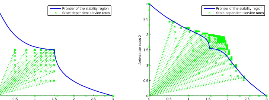
number of users due to multiuser diversity. Figure 1 shows the service rate vectors for various numbers of users in each cell, and the frontier of the stability region for two types of allocation functions φ(·) and ψ(·) given by:
φi(n) = min(3,log(1 +ni))(1nj>0+ 0.5·1nj>0), j6=i,
ψi(n) = min(3,log(1 +ni))
1
2−(1 +j)−0.4, j 6=i.
In the first scenario, the interference reduces the service rates by a factor 2 as soon as the number of users in the interfering cell is strictly positive. In the second case, the interference is smoother and the impact on the service rates increases with the number of active users in the interfering cell.
The resulting stability regions are not convex and depend in a complicated way on the tradeoff between interference and the gain from channel-aware scheduling. Note that operating the network in the most symmetric fashion (equal arrival rates in each cell) is optimal in the first scenario but not in the second case where the arrival rates maximizing the total traffic that the network can support are non-trivial.
0 0.5 1 1.5 2 2.5 3 0 0.5 1 1.5 2 2.5 3
Arrival rate class 1
Arrival rate class 2
Frontier of the stability region State dependent service rates
0 0.5 1 1.5 2 2.5 3 0 0.5 1 1.5 2 2.5 3
Arrival rate class 1
Arrival rate class 2
Frontier of the stability region State dependent service rates
Figure 1: State-dependent service rates and the corresponding stability region.
With an arbitrary number of K user classes, the global stability region involves K! sets of conditions in general. However, depending on the topology and possible symmetries, the number of conditions can possibly be reduced. Consider for example a 3-cell linear network. Suppose that cell 1 is in the middle and interferes with cells 2 and 3, while cells 2 and 3 interfere only with cell 1. To simplify notation, denote byφAi the service rate received by celli
when cells outside A ⊆ {1,2,3} are supposed to be saturated and cells in A are supposed to be stationary. The stability conditions boil down to:
λ1< φ∅1, λ2< φ {1} 2 , λ3 < φ {1} 3 , orλ2< φ∅2, λ1< φ1{2}, λ3 < φ{31}, orλ2 < φ∅1, λ3 < φ3∅, λ1 < φ{12,3}, orλ3< φ∅3, λ1< φ1{3}, λ2 < φ{21}.
The proof of Propositions 3.1 and 3.2 developed in [24] relies both on stochastic comparisons and martingale arguments, and does not involve specific Lyapunov functions. The knowledge of a Lyapunov function provides however valuable insight into the type and speed of convergence of the process to its stationary distribution [51]. Following [39], we now give a construction of a Lyapunov function in the simplest case of two user classes. The construction sheds some light on the difficulty of making such functions explicit, as they should depend on the specific properties of the allocation function φ(·). The construction of the Lyapunov function relies on solving a Poisson equation. For that purpose, suppose without loss of generality that
λi+φi(n)<1,i= 1,2, for alln∈N2 and define P as the kernel of a one-dimensional Markov
process with transition rates
p(n1, n1+ 1) =λ1, p(n1, n1−1) =`1φ1(n1), p(n1, n1) = 1−(λ1+`1φ1(n1)).
Proposition 3.3 If
λ1< `0φ1 and λ2 < L12(λ1),
then a Lyapunov function for the system is given by
F(n) :=ψn1 +γ[n
2+V(n1)].
with ψ > 1, γ > 0 some constants to be chosen and V(·) a bounded function defined as the solution of the Poisson equation (I−P)V =λ2−`1φ2+, with:=L12(λ1)−λ2.
3.3 Bounds for the stability conditions and performance
In this subsection, we use further stochastic comparisons to derive bounds for the stability conditions and the performance that are far simpler to compute. Recall that Yl(t) is the
l-dimensional birth-death process with birth rates λi and death rates `lφi, i= 1, . . . , l. The
partial monotonicity of the allocation function implies that (N1, . . . , Nl)≤st(Y1l, . . . , Yll).
This stochastic comparison has yielded the stability conditions in Proposition 3.1. However, the stability conditions obtained can be difficult to compute, since they involve the calculation of the stationary distribution πl of the l-dimensional process Yl(t), which does not have a
closed form in general unlessl= 1. Using the fact that`lφi is partially decreasing,i= 1, . . . , l,
however, we can derive a looser stochastic comparison, namely (N1, . . . , Nl)≤st (Y1l, . . . , Yll)≤st( ˜Y1l−1, . . . ,Y˜l
−1
l−1,N˜l), (4)
where the process ( ˜Yl−1,N˜l) has death rates φi
i(ni),i= 1, . . . , l−1, and`lφl, with
φii(ni) = lim
r→∞nj>r,jinf6=i
φi(n1, . . . , nK).
Note that with these modified death rates, the processes ˜Yj = ( ˜Y1j, . . . ,Y˜jj) are themselves Markov processes for all j. Moreover, all their components decouple, leading to the following stationary distribution ˜ πj(n1, . . . , nj) := 1 Gj j Y i=1 ni Y mi=1 λi φii(mi) , withGj :=P n1,...,nj∈Nj Qj i=1 Qni mi=1 λi φi i(mi).Defining ˜ Lii−1(λ1, . . . , λi−1;φ) := X n1,...,ni−1 `i−1φi(n1, . . . , ni−1)˜πi−1(n1, . . . , ni−1),
we obtain the following simple sufficient stability condition.
Proposition 3.4 Ifλj <L˜j −1
i (λ1, . . . , λi−1;φ)for allj = 1, . . . , l, then the process(N1(t), . . . , Nl(t))
is stable.
ProofBy virtue of the stochastic dominance and the fact that the allocation function φ(·) is partially decreasing, we obtain
X
n1,...,ni−1
`i−1φi(n1, . . . , ni−1)˜πi−1(n1, . . . , ni−1)≤Lii−1(λ1, . . . , λi−1;φ).
Thus the condition in (3) is implied by the inequalityλi <L˜ii−1(λ1, . . . , λi−1;φ). 2
Remark 3.2 Note that the bounds are insensitive to the flow size distribution. Also, the bounds coincide with the exact stability conditions in case of two user classes.
Remark 3.3 Note that the bounds extend to scenarios with several user classes per cell, as long as the correlations between service rates depend on the total number of users per cell only.
Using (4), the number of users (of classk, say)Nkcan be bounded by a process ˜Nkhaving death
rates`kφk( ˜Yk−1,N˜k), where ˜Yk−1has been defined above and is not influenced by ˜Nk. Here we
would index the classes in such a manner that classkinterferes with classes 1, . . . , k−1, but not with classesk+1, . . . , K. Unfortunately, this does not lead directly to closed-form bounds. The difficulty arises from the fact that ˜Nk behaves as a birth-death process driven by a random
environment ˜Yk−1, which is intractable in general. Hence, we introduce approximations of the bounds along the lines of [14, 32], based on two limit regimes, termed fluid and quasi-stationary, where the process ˜Yk−1 evolves on an infinitely fast and an infinitely slow time scale, respectively. Specifically, we consider a family of systems, parametrized by s∈ (0,∞) and obtained by accelerating the process ˜Yk−1(t) by a factor s, i.e., replacing the process
˜
Yk−1(t) by ˜Yk−1(s×t).
Quasi-stationary regime The quasi-stationary regime is obtained when the acceleration factorstends to 0. In the limit fors→0, the process ˜Yk−1(t) is frozen to its initial state. Thus the quasi-stationary regime corresponds to a scenario where the process ˜Yk−1(t) is constant and equal to (n1, . . . , nk−1) with probability ˜πk−1(n1, . . . , nk−1).
Assuming λk <inf(n1,...,nk−1)∈Nk−1lim infnk→∞` kφ
k(n1, . . . , nk−1, nk), we obtain the
distribu-tion of the number of active class-k flows in the quasi-stationary regime:
pqsk (nk) = X (n1,...,nk−1)∈Nk−1 ˜ πk−1(n1, . . . , nk−1)p qs k (nk|n1, . . . , nk−1), with pqsk (nk|n1, . . . , nk−1) =G qs k (n1, . . . , nk−1) nk Y m=1 λk `kφ k(n1, . . . , nk−1, m) , and Gqsk (n1, . . . , nk−1) := P∞ n=0 Qn m=1 λk `kφ( kn1,...,nk−1,m) −1 .
Fluid regime The fluid regime is obtained when the acceleration factor s tends to ∞. In the limit for s → ∞, the process ˜Yk−1(t) evolves so rapidly that when there are n
k class-k
users, their total service rate is constant and equal to ¯ φflk(nk) = X (n1,...,nk−1)∈Nk−1 ˜ πk−1(n1, . . . , nk−1)`kφk(n1, . . . , nk−1, nk).
Assumingλk<lim infnk→∞φ¯
fl
k(nk), we derive the distribution of the number of active class-k
flows in the fluid regime
pflk(nk) =G fl k nk Y m=1 λk ¯ φflk(m) , withGflk := P∞ n=0 Qn m=1 λk ¯ φflk(m) −1 .
A question of importance is whether these quasi-stationary and fluid regimes provide actual bounds for the orginal upper bounds. From studies on single-class PS queues with time-varying capacity [32], the performance in the quasi-stationary (resp. fluid) regime is worse (resp. better) than that of the actual system. Numerical results in [7] lend further support to that observation. Thus, the quasi-stationary regime of the upper bound ˜Nk is likely to be an upper bound for the actual number of active flows Nk.
4
Intra- and inter-cell mobility
So far we have assumed that the rate variations occur on a fast time scale and average out over the time scale of interest for flow-level performance, only manifesting themselves in the throughput gains obtained from channel-aware scheduling. We now turn attention to a scenario where the fluctuations may have a slowly varying component. This component may correspond to the variations in the channel attenuation between BS’s and users due to user mobility. In order to simplify the presentation, we ignore fast fading unless otherwise specified. The results presented in this section can be readily extended to account for fast fading. We no longer include time-varying inter-cell interference. Finally, we assume that the scheduling strategies operate on a faster time scale (of the order of ms) than that of user mobility (of the order of several seconds). The results presented in this section offer a summary of those in [8, 21, 22].
4.1 Mobility model
In order to model user mobility, it is convenient to adopt a ‘state structure’, with the users moving among several possible states indexed by a finite setI. The states implicitly correspond to geographic subregions of the network. The latter is divided into a set B of cells, and we denote byIb the set of states corresponding to subregions in cellb, i.e., where users are served by BS b. When in state i∈ Ib, a user is served at rate Ci when scheduled by BS b.
We categorize users according to their mobility. Specifically, we consider a system withKtraffic classes. We denote byXkm(t) the state of them-th arriving class-kuser, and by Fkm its flow
size. (For notational convenience, we define Xkm(t) for all values oft. Note however that the
m-th class-k user may not have arrived yet or may already have departed at time t, in which case Xkm(t) is inconsequential.) We assume that Fkm and Xkm(t), m = 1,2, . . ., are i.i.d.
copies of an exponential random variable Fk with mean ξk and a Markovian stationary and
ergodic process Xk(t) with state space I, respectively. Denote by Rk(t) = CXk(t) the generic rate process for classk. Define πi,k :=P{Xk(t) =i} as the stationary probability for a class-k
user to be in state i, and Jk := {i ∈ I : πi,k > 0} as the set of states in which a class-k
user may reside. Define pk,b :=Pi∈Ibπi,k as the stationary probability that a class-k user is in cell b. Finally, denote by Bk := {b ∈ B :pk,b > 0} the set of cells that class-k users may
visit. Users of classes 1, . . . , K generate flows according to independent Poisson processes of intensitiesλ1, . . . , λK, respectively, and we denote by σk:=λkξk the traffic intensity of class-k
users.
We first provide stability conditions that depend on the scheduling strategy, and then derive bounds for the transfer delays using stochastic comparison methods.
4.2 Stability
We now determine the set of all traffic vectors (σ1, . . . , σK) such that the system is stable.
This set depends, as we will see, on the underlying scheduling strategy. We first investigate strategies that maximize the stability region, and then considerα-fair schedulers.
4.2.1 Optimal scheduling strategies
We first determine the capacity region for optimal scheduling strategies. In other words, we characterize the set of all traffic vectors (σ1, . . . , σK) for which there exists a scheduling strategy
that achieves stability. Define:
T := {(τi,k)i∈I,k=1,...,K ∈R+(|I|×K):τi,k = 0 if i6∈ Jk, and K X k=1 X i∈Ib∩Jk τi,k = 1,∀b∈ B}, R := {(r1, . . . , rK)∈RK+ :∃τ ∈ T such that rk≤ X i∈I τi,kCi,∀k= 1, . . . , K}.
The component τi,k,i∈ Ib, may be interpreted as the fraction of resources of BS b allocated
to class-k users in statei. With that interpretation, the quantity P
i∈Iτi,kCi represents the
total service rate received by class-k users. Thus,Rmay be interpreted as the achievable rate region, i.e., the set of all achievable service rates for the various traffic classes.
Note that Ris a convex set and depends on the spatial user distributions through the setsJk
only.
Proposition 4.1 There exists a scheduling strategy that achieves stability if (σ1, . . . , σK) ∈
int(R). Conversely, if (σ1, . . . , σK)6∈ R, then there exists no scheduling strategy that achieves
stability.
Proof Assume (σ1, . . . , σK) ∈ int(R). Then there exists a vector (τi,k)i,k ∈ T such that
σk < P
i∈Iτi,kCi for allk= 1, . . . , K. Now consider a static scheduling strategy that allocates
in cellb a fixed fraction τi,k,i∈ Ib of the resources to class k in that cell. By considering the
system in the fluid limit, it can be shown that this strategy achieves stability. The converse statement follows from the convexity of R. If (σ1, . . . , σK)∈ R/ , then by convexity of R, there
exists a linear hyperplaneHcontaining (σ1, . . . , σK) defined byPKk=1akσk=d, withak, d >0,
such that there exists an >0 with PK
k=1akrk < d−for all rate vectors (r1, . . . , rK) ∈ R.
Thus, in the fluid limit, the quantityPK
k=1akn¯k(t), where ¯nk(t) is the number of active class-k
users at time t in the fluid limit, will continuously grow at least at rate , which implies that
the system is unstable. 2
Example 4.1 (Single traffic class) If there is just a single traffic class, i.e., K = 1, then, dropping the class index k, R = {r ∈ R+ :∃τ ∈ T such that r < P
i∈IτiCi}, which may be
represented in a more compact manner as R= [0, rmax), with rmax:=
P
b∈Bmax i∈Ib
Ci.
Example 4.2 (Intra-cell mobility only) If there is intra-cell mobility only, i.e., each of the setsBk is just a singleton, thenR={(r1, . . . , rK)∈RK+ :
P k:Bk={b}
rk/Ckmax≤1,∀b∈ B}, where
Ckmax:= max
i∈Jk
Ci denotes the highest transmission rate of class-k users.
Note that in both the above two examples the BS only serves classes in their most favorable state within the cell.
4.2.2 α-fair resource sharing
We now assume that each BS implements anα-fair scheduling discipline, independently of the behavior of other BS’s. Thus when there areni,k class-k users in state i,i∈ Ib, each of them
receives service at rate C
1/α i PK l=1 P j∈Ibnj,lC1/α −1 j .
Define Rα := {(r1, . . . , rK)∈RK+ :∃θ∈RK+ such that rk≤ X b∈B P i∈Ibπi,kθkC 1/α i PK l=1 P j∈Ibπj,lθlC 1/α−1 j ,∀k= 1, . . . , K}.
Note that the vector (τi,k) with τi,k =
πi,kθkC1/α −1 i PK l=1 P j∈Ibπj,lθlC1/α −1 j
, i∈ Ib, belongs to the set T, so thatRα ⊆ R.
The components of the vector (θ1, . . . , θK) may be interpreted as the numbers of flows of the
various classes. With that interpretation, the quantity P b∈B P i∈Ibπi,kθkC 1/α i PK l=1 P j∈Ibπj,lθlC 1/α−1 j represents the total service rate received by class-k flows under anα-fair sharing strategy.
The regionRα has a non-linear boundary in general, and may either be convex or non-convex,
depending on the values of the probabilities πi,k and the rates Ci, see Example 4.5 for a
graphical illustration.
The next proposition provides a characterization of the capacity region in case ofα-fair resource sharing, assuming exponential service requirements. It states that the system is stable if and only if there exists a relative distribution of the numbers of flows across the various classes so that the total service rate received by each of the traffic classes is larger than the traffic intensity of that class.
Proposition 4.2 If (σ1, . . . , σK) ∈int(Rα), then the system is stable. If (σ1, . . . , σK) 6∈ Rα,
then the system is unstable.
Proof The proof relies on the consideration of fluid limits [31], where systems with a large population of flows are considered. In such limiting systems, it can be shown that the total service rate received by class-kflows is given by:
rk(t) = X b∈B ¯ nk(t)Aαk,b PK l=1n¯l(t)Bl,bα , (5)
for ¯nk(t)>0, and where
Aαk,b= X i∈Ib πi,kCi1/α, Bk,bα = X i∈Ib πi,kC1/α −1 i .
In the above formula, ¯nk(t) denotes the number of class-k flows at timet. The proof of (5) is
standard when a single cell is considered, but involves a spatial homogeneity property in the case of networks with several cells. Intuitively, one can justify this formula by observing that when the number of class-k flows is very large then at any instant, the number of such flows in stateishould beπi,kn¯k(t). This statement can be formally justified as in [56].
The evolution of the fluid limit is characterized by the following set of differential equations:
∀k, d
dtn¯k(t) =λk−µk×rk(t),
whereµk:= 1/ξk.
Assume that (σ1, . . . , σK)∈int(Rα). Then there exists a vector (θ1, . . . , θK)∈RK+ such that λk< µk P b∈B θkAαk,b PK l=1θlBl,bα
−for >0 sufficiently small for all k= 1, . . . , K. We now consider the quantity y(t) := maxk=1,...,Kn¯k(t)/θk and show that it will continuously decrease at a
strictly negative rate.
Denotek∗:= arg maxk=1,...,Kn¯k(t)/θk, where the implicit dependence ontis suppressed. Then:
d dtn¯k∗(t) =λk∗−µk∗ X b∈B ¯ nk∗(t)Aα k∗,b PK l=1n¯l(t)Bl,bα =λk∗−µk∗ X b∈B Aαk∗,b PK l=1Bl,bαn¯l(t)/n¯k∗(t) < λk∗−µk∗ X b∈B Aαk∗,b PK l=1Bl,bαθl/θk∗ =λk∗−µk∗ X b∈B Aαk∗,bθk∗ PK l=1Bl,bαθl < ,
whenever ¯nk∗(t) >0. We conclude that the fluid limit reaches zero in finite time, and hence
the system is stable [31]. Necessary stability condition
Denote by ∂Rα the boundary of Rα, i.e., r ∈ ∂Rα if r ∈ Rα and there exists a k such that
∀ > 0, r+.ek ∈ R/ α. This boundary is the union of the surfaces ∂RαL over all non-empty subsets Lof {1, . . . , K}, with: ∂RαL= r∈RK+ :∃θ∈R+|L|,∃θ0∈R|+L|¯, ∀k∈ L, θk>0, rk = X b∈B θkAαk,b P l∈LθlBl,bα , ∀k∈L¯, rk≤ X b∈BL θk0Aαk,b P l∈L¯θl0Bl,bα ,
where ¯L={1, . . . , K} \ LandBLdenotes the set of cells that are not visited by users of classes in the set L. The surface ∂Rα
L is the set of points of Rα parametrized by θsuch that ∀k∈ L,
∀l∈L¯, θk θl. It is worth remarking that ∂RαL is part of a cylinder with directions parallel to the components in ¯L, i.e., if r is a point of this surface, thenr0 = (rk, k∈ L, rl0, l∈ L¯) is
also a point of this surface provided that for all l ∈ L¯, 0 ≤ r0l ≤ rl. It is also important to
note that in the definition of ∂Rα
L, we can chooseθ ∈R |L|
+ with strictly positive components;
this is because the points obtained when some of the components of thisθ are equal to 0, are included in some other surfaces with a different setL.
We now prove that the system is unstable by induction on the numberK of flow classes. The result holds forK = 1. Assume that it is true for all systems with at mostK−1 classes. Let us prove it in the case ofK-class systems. Assume thatσ = (σ1, . . . , σK)∈ R/ α. Without loss
of generality, we can assume that σk >0 for all k= 1, . . . , K. Now defineγ as the maximum
real number such that γ×σ ∈ Rα. By assumption, γ <1. Of course, we have γ×σ ∈∂Rα,
and there exists a set of classes L such thatγ×σ ∈∂Rα
(i) If L = {1, . . . , K}, then we deduce that there exists θ ∈ RK
+ such that θk > 0 for all
k= 1, . . . , K and: σk> X b∈B θkAαk,b PK l=1θlBl,bα .
We deduce that the system is unstable. Indeed one can easily show that the fluid limit grows at least linearly to∞.
(ii) Otherwise, we consider the restricted system where the classes in ¯L have no traffic. Note that the restricted system provides a stochastic lower bound of the actual system (this is due to the fact that all the systems considered are monotonic [14]). Hence we just need to prove that the restricted system is unstable. Note that the projection of∂Rα
L on the sub-space ofL components is actually the boundary of the setRα
L defined by: RαL= r∈R|L|+ :∃θ∈R|L|+ ,∀k∈ L, rk≤ X b∈B θkAαk,b P l∈LθlBl,bα . Since ∂Rα
L is a cylinder, we deduce that (σk, k ∈ L) ∈ R/ αL, and finally that the restricted
system is unstable by induction. 2
Example 4.3 (Single traffic class) If there is just a single traffic class, i.e., K = 1, then
Rα= [0, rα
max) with, dropping the class indexk, rαmax:=
P b∈BCb, with Cb:=Pi∈IbπiC 1/α i / P j∈IbπjC 1/α−1 j .
Example 4.4 (Intra-cell mobility only) If there is intra-cell mobility only, i.e., each of the sets Bk is just a singleton, thenRα ={(r
1, . . . , rK) ∈RK+ : P k:Bk={b} rk/Ckave≤1,∀b∈ B}, where Cave k := P
i∈Jkπi,kCi denotes the average rate coefficient of class-k flows.
In both the above two examples it is easily seen that the capacity region Rα decreases when
the value of the fairness indexα increases, which in fact holds in greater generality as will be shown in Proposition 4.3 below.
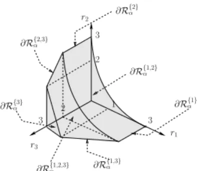
Example 4.5 (A 3-cell 3-class network) In general, the capacity regionRα has non-linear
boundaries and its shape turns out to be rather intricate. We present an example of a three-cell three-class network to illustrate how astonishing this shape can be. There are five states, with
C1 = C4 = C5 = 2, C2 = C3 = 1, I1 = {1,2}, I2 = {3,4}, and I3 = {5}. Class-1 users
oscillate between states 1 and 3 with probability 0.1 to be in state 1, class-2 users between states 2 and 4 with probability 0.9 to be in state 2, and class-3 users between states 2 and 5, with equal probability to be in each state. Figure 2 depictsR1, i.e., the capacity region for the
PF strategy, and indicates the various surfaces ∂RL1 composing the boundary ofR1.
4.2.3 Impact of scheduling
It is worth observing that the stability regionRα depends on the fairness indexα, i.e., on the
scheduling discipline, even in the simple case of single-cell single class systems. This contrasts with the case where users are not moving (see§4.2.4). The next proposition, whose proof can be found in [22], states that the stability region actually grows monotonically as the value ofα
decreases.
r3 3 3 2 2 1 ∂R{1,2} α ∂R{1,3} α ∂R{2,3} α r1 ∂R{α1} ∂R{1,2,3} α ∂R{α3} 3 ∂R{2} α r2
Figure 2: Capacity region R1 of a three-cell three-class network with mobility under the PF
strategy.
4.2.4 Mobility increases stability
Let us first provide the stability region in the case where users are not moving, i.e., the state of a user is assumed to be fixed for the duration of the flow, and the probability that a class-k
user is in stateiisψi,k. Consider systems where the scheduling discipline implemented at each
BS is arbitrary but work-conserving, i.e., each BS is active whenever there is a user in the corresponding cell. It can be easily shown that the stability region without mobility does not depend on the scheduling discipline and simplifies to
Rno :={(r1, . . . , rK)∈RK+ :∃τ ∈ T such that ψi,krk< τi,kCi,∀i∈ I, k= 1, . . . , K},
which may be represented in a more compact manner as
Rno ={(r1, . . . , rK)∈RK+ : K X k=1 X i∈Ib ψi,krk/Ci <1,∀b∈ B}.
To compare the stability regions with and without mobility, it makes sense to assume that for all k, i, πi,k = ψi,k. The next proposition first states that the stability region with mobility
is larger than that without mobility as long as the scheduling discipline is left flexible, which agrees with findings in the context of ad-hoc mobile networks [35]. It further states that this observation also remains valid forα-fair scheduling strategies. Its proof can be found in [22].
Proposition 4.4 We have:
Rno ⊆ R, and for any α >0, Rno ⊆ Rα.
4.3 Transfer delays
With user mobility, the network may be interpreted as a system of (PS) queues with state-dependent and time-varying capacities, and not surprisingly, it proves impossible to obtain exact expressions for the transfer delays (even the average values). In this subsection, we develop a method, based on stochastic comparison techniques, to derive upper and lower bounds for transfer delays. We restrict our attention to intra-cell mobility, and consider the class of schedulers such that the service rate of a class-k user in statei is of the form:
where as before nk denotes the number of active class-k users. For any k, the function
Hk(·) is decreasing in each of the nj’s, j = 1, . . . , K. Note that the above form does not
apply for α-fair schedulers, except the PF strategy (α = 1), for which Hk(n1, . . . , nK) =
G(PK
k=1nk)/( PK
k=1nk). For general α-fair schedulers, we believe that the results remain
valid, but the proof will require a different approach.
4.3.1 Limiting regimes
In order to obtain tractable performance estimates, we introduce two limit regimes, termedfluid and quasi-stationary regime, where the rate processes evolve on an infinitely fast and an in-finitely slow time scale, respectively. Formally, let us consider a family of systems, parametrized by s ∈ (0,∞), where the generic rate process for class k is Rk(s)(t) := Rk(st). Thus the
pa-rametersrepresents the ‘speed’ of the rate process. Or equivalently, the value 1/smodels the time scale of the rate process. In the case whereXk(t) is a Markov process, the processR(ks)(t)
may be obtained by scaling the transition rates with s.
When the parametersgrows large, the rate process approximately averages out over the time scale of the flow dynamics. In the limit fors→ ∞, the variations completely vanish, and the rate process reduces to a constant, giving rise to the ‘fluid’ regime withRfl
k(t) :=R
(∞)
k (t) = ¯Rk,
where ¯Rk := E{Rk(0)}. It is worth observing that the fluid regime is reminiscent of (but
different from) the usual law-of-large-numbers fluid limit. On the other hand, as the value ofsbecomes small, the fading process remains roughly constant over the time scale of the flow dynamics. In the limit fors→0, the changes completely disappear, and the rate process freezes in some initial state, yielding the ‘quasi-stationary’ regime with Rqsk(t) := R(0)k (t) = Rk(0),
whereRk(0) has the stationary marginal distribution of the process Rk(t).
For example, for the PF strategy, the fluid and quasi-stationary regimes yield tractable ex-pressions for the transfer delays. Define the traffic intensities associated with class k in the fluid and quasi-stationary regimes asρflk:=λkξk/R¯k and ρqsk :=λkξkE{1/Rk(0)}, respectively.
Note that these values depend on the rate statistics only through the arithmetic and harmonic means, respectively. By Jensen’s inequality, we have ρflk ≤ρqsk . Denote by ρfl :=PK
k=1ρflk and
ρqs := PK k=1ρ
qs
k the total traffic intensities in the fluid and quasi-stationary regimes,
respec-tively. With the above translation to a multi-class PS system (without time-varying capacities), the performance in the fluid and quasi-stationary regimes may be explicitly evaluated using results of Subsection 2.1. In particular, a necessary and sufficient condition for stability of the fluid (respectively, quasi-stationary) regime is ρfl < G∗ (respectively, ρqs < G∗). When the system is stable, the stationary distributions πfl and πqs of the numbers (n1, . . . , nK) of
active flows of the various classes in the respective regimes depend on the class characteristics through the traffic intensitiesρflk and ρqsk , respectively, only:
πfl(n1, . . . , nK) =πfl(0) n φ(n) K Y k=1 (ρflk)nk nk! , πqs(n1, . . . , nK) =πqs(0) n φ(n) K Y k=1 (ρqsk)nk nk! , wheren:=PK k=1nk,φ(n) := n Q i=1
G(i), andπfl(0) andπqs(0) are determined by the respective normalizing conditions.