Estimating Design Time for System Circuits

Estimating Design Time for System Circuits

Cyrus Bazeghi Francisco J. Mesa-Mart´ınez Brian Greskamp

_{Josep Torrellas}

_{Jose Renau}

Dept. of Computer Engineering, University of California Santa Cruz http://masc.soe.ucsc.edu

†

Dept. of Computer Science, University of Illinois at Urbana-Champaign http://iacoma.cs.uiuc.edu

ABSTRACT

System design complexity is growing rapidly. As a result, cur-rent development costs are constantly increasing. It is becom-ing increasbecom-ingly difficult to estimate how much time it will take to design and verify these designs, which are getting denser and increasingly more complex. To compound this problem, circuit design cost estimation still does not have a quantita-tive approach. Although designing a system is very resource consuming, there is little work invested in measuring, under-standing, and estimating the effort required.

To address part of the current shortcomings, this paper in-troducesµPCBComplexity, a methodology to measure and es-timate PCB (printed circuit board) design effort. PCBs are the central component of many systems and require large amounts of resources to properly design and verify. µPCBComplexity

consists of two main parts; a procedure to account for the contributions of the different elements in the design, and a non-linear statistical regression of experimental measures in order to determine a good design effort metric. We use µPCBComplexity to evaluate a series of design effort es-timators for twelve PCB designs. By using the proposed µPCBComplexitymetric, designers can estimate PCB design effort.

1

Introduction

Printed circuit board (PCB) design effort keeps growing due to such constraints as rising clock frequencies, thermal issues, reduced area, increasing number of layers, mixed signal de-vices, and the ever increasing component count and density. All of these factors combined have led to a steady rate of in-crease in development costs for current systems. As we design ever larger, denser and more complex systems, it is becoming increasingly difficult to estimate how much time would be re-quired to design and verify them. To compound this problem, PCB design effort estimation still does not have a quantitative approach. We present in this paper a first step toward creating a design effort metric that is highly correlated with design ef-fort for PCB layout. We follow a similar approach taken in [1] as the principles that are applicable to microprocessors are also This work was supported in part by the National Science Foundation under grants 0546819 and 720913; Special Research Grant from the University of California, Santa Cruz; and gifts from SUN.

applicable to PCBs. In this paper, design effort corresponds to the number of engineering-hours required for implementation (layout) of a PCB design.

This paper analyzes and proposes various statistics to esti-mate the layout effort required to develop PCBs. We inves-tigate and quantify statistics such as area, component count, pin count and device types and sizes for many PCBs. We ana-lyze several of these statistics, and propose a metric, obtained after applying non-linear regression over the different statis-tics, which we callµPCBComplexity. In addition, we provide insights on the correlation between several statistics and the design effort for many systems with known layout times.

Different designs have different constraints, leading to spe-cific challenges; typical design constraints being area, fre-quency, and manufacturing cost. For example, having area being a primary design constraint, may lead to a requirement for additional layers, more expensive package types, and more complex placement and routing. A design constrained by cost, on the other hand, may require a balance between number of layers, area, drill density, types of packages and possibly the number of different drill sizes. Having clear constraints is nec-essary in estimating layout effort as it can drastically affect complexity.

We define design effort to be the required time in man-months to produce the layout for a given system. Design effort is equivalent to layout time when the project has a single devel-oper, which is frequent even for complex PCBs. Nevertheless, for a given effort requirement, it is possible to reduce the de-sign time by increasing the number of workers. Nevertheless, increasing the number of workers decreases the productivity per worker. The relationship between these two elements has been widely studied in software metrics and business models. Since the conversion between design effort and design time can be approximated, the remainder of this paper focuses only on design effort.

The rest of the paper is organized as follows. Section 2 covers other work in this area; Section 3 describes the sta-tistical techniques that allow us to calibrate and evaluate the µPCBComplexity regression model; Section 4 describes the setup for our evaluation; Section 5 evaluates several statistics for the boards in our analysis; and Section 6 presents conclu-sions and future work.

2

Related Work

The capability to rapidly develop complex PCBs is a tremen-dous competitive advantage, since high development produc-tivity is essential for the success of any design team. Although some companies have used statistical methods to estimate PCB design time, those methods are considered trade secrets [9]. Other companies do not release details because they provide competitive advantage over other companies. As a result, we are unaware of any published work on the topic of predicting the engineering hours required for a PCB design.

[1] focuses on microprocessor design effort. While the work described in this paper focuses on PCB design metrics, [1] uses a similar regression model, but both papers analyze different sets of statistics and targets.

There exists some published work that aids in the layout ef-fort. A useful model for wiring density is called “Rent’s rule”, after an IBM engineer who popularized it [7]. This model at-tempts to calculate the required trace spacing on a board using the dimensions, number of routing layer, and the number of connections (assuming they are distributed according to Rent’s rule).

Another paper that looks at productivity is [6] which iden-tifies the need for standards or infrastructures for measuring and recording the semiconductor design process. They propose improving design technology, time-to-market, and quality-of-result by addressing the Design Productivity Gap and the De-sign ”Technology” Productivity Gap. However, this previous work focused mostly on the problems associated with the in-frastructure and design tools related to the physical implemen-tation of semiconductor designs, while the focus of this paper is layout effort associated with PCB designs.

In [8] a factor similar to the productivity factor is described. They use the “process productivity parameter” to tune the es-timating process for software projects. They contend that if you know the size, time, and the process productivity parame-ter you can use it to make estimates for a new project. So long as the environment, tools, methods, practices, and skills of the people have not changed dramatically from one project to the next.

Much research has been done in Design for Manufacturing (DFM) and Design for Production (DFP) which attempts to improve the production and manufacturing times of PCB as-semblies. This paper seeks to develop a metric that can aid in predicting the layout effort, based on analysis of characteristics of PCBs at a low-level so as to better plan for future generations of systems. In [2] the issue of embedded passive components is discussed as a necessity to the smaller electronic devices re-quiring ever smaller PCBs. They note that board area is be-coming so critical that to keep pace with the size constraints new techniques are required. Our goal would be to eventually develop a set of metrics and a model that estimates design ef-fort by also taking into account manufacturing times.

3

Approach

The goal of this paper is to develop not only a quantitative ap-proach but also produce a model that quickly estimates design effort based on several easily gathered statistics. This is impor-tant because being able to predict design effort is advantageous in helping to reduce design costs. To build the model, we ana-lyze many commercial computer/electronic devices and gather data from their PCBs. The layout times for these PCBs were well documented which was a requirement for this analysis. Table 1 lists the critical components of PCB designs as deter-mined by [2]. These parameters contribute to the complexity of a design, and hence the time required to do layout.

1. Board dimensions (length and breadth) 2. Total wiring requirements

3. Number of layers

4. Number of embedded resistors (if used) 5. Number of embedded capacitors (if used) 6. Set of active component types and their number 7. Thickness of the board

8. Number of discrete resistors 9. Number of discrete capacitors

Table 1:Critical design parameters for a PCB.

Some design parameters listed in Table 1 are dependent on other factors. For example, the size of the board is defined by the number of embedded and discrete passive components and total wiring requirements. However, the total wiring require-ments are governed by the number of embedded and discrete passive components in the PCB. And further more, the total number of layers in the PCB depends on the size of the board, the number of embedded and discrete resistors and bypass ca-pacitors [2].

These critical design parameters are focused towards man-ufacturability, not design effort estimation. We used them as a starting point in determining what parameters or metrics to analyze and include for correlation with design effort. None of the boards in our study have embedded passive components; instead we focus on the total number of all components (pas-sive and discrete) and the pin count for them. These are easily obtainable values.

Since the routing data is not easily obtainable, the number of pins for all the components in the design is taken into account instead. While this is not an ideal metric since not all pins are used or have very short traces (VDD or GND), it is readily obtainable and does not hamper the focus of this paper, namely effort prediction starting from higher level design descriptions, such as a bill of materials (BOM) or schematics.

In order to find a metric highly correlated with design effort, several statistics were gathered from the existing designs. For each isolated board with a known design effort, we look at sev-eral statistics and apply non-linear regression to find a highly correlated metric.

of statistics (Si). Each of which has a specific constant (wi),

associated with it, which assigns a weight to the importance of every statistic used as input in the model. The aggregate of the statistics is inversely proportional to the productivity of a specific design team which is represented by a constant (ρ). The model is presented in Equation 1. In order to find suitable values for each of the data weights (wi) we perform mixed

non-linear regressions on this equation. The design team pro-ductivity factor (ρ) is constant per design group, and it needs to be adjusted on a per company or design team basis. If theρis unknown, then the absolute design effort is invalid and only the breakdown inside the project is correct. Obtaining the value of ρis simple; all that is needed is to have the design effort for a single project. Alternatively, it is possible to develop a produc-tivity benchmark suite that calibratesρfor a given company.

Design Effort=1 ρ × n X k=1 (wk×S_k) (1) In order to determine the weights that give a generalized so-lution to Equation 1, [1] proposes to use a mixed non-linear regression model. If there are no productivity adjustments, it is possible to use a simpler non-linear regression model. While the sum of a large number of random variables is distributed normally, the product of a number of random variables is dis-tributedlognormally— a distribution where the logarithm of the variable is normally distributed [3]. Therefore, since the random variables have a log normal distribution an even sim-pler linear regression model can not be used.

To evaluate the accuracy of the model (Section 5), we use σas a measure of error associated with the fit. Consequently, it is important to understand what different values ofσtell us about the quality of the estimate. For a givenσ, we can find aconfidence intervalfor the estimated effort. Thex% confi-dence interval for a metric is defined to be the range of efforts (Estimatelow, Estimatehigh)such that P(Estimatelow <

metric prediction< Estimatehigh) = x/100. For example,

the 90% confidence interval gives us two valuesaandbsuch that there is a 90% chance that the actual effort is between metric prediction×aand metric prediction×b.

3.1 Productivity Adjustments

In software development projects, it is well known that differ-ent developmdiffer-ent teams have differdiffer-ent productivities. For ex-ample, it has been shown that the productivity difference tween teams can be up to an order of magnitude [4]. We be-lieve that a similar effect occurs between PCB design teams. The productivity differences may be due to multiple factors, including the average experience of the designers in the team and the tools used. In our model,ρcaptures this effect.

The boards under study in this analysis either all came from one manufacturer, or we only had one board from the manu-facturer, so the use of a productivity factor was not necessary.

3.2 Team Size Dynamics

Although some board designs require long periods of time, it is very rare to find multiple developers doing different sections of the same board. The PCB layout effort by nature is a lin-ear task done by one engineer at a time. To reduce the design time, we have found two approaches: multi-timezone working environments, and ”surgical” teams.

A multi-timezone team has different designers working in multiple time zones, this is, once a designer stops working a new designer can continue and pick up where the previous de-signer left. A “surgical team” [5] follows an alternative design organization, with the surgeon, or chief designer, at the helm and a supporting staff that has their tasks allocated by the chief of staff. In the PCB case, we may have other designers doing such tasks as making footprint images for components, which can be a tedious effort.

3.3 R-Language

This section provides the R-language [10] code to fit the non-linear mixed-effects model and the non-linear regression model. The mixed-effects model is needed when productivity adjustments (ρ) are required, a simpler model is used when no productivity adjustments are required.

Recall that our model has a multiplicative lognormal error and also a lognormal distribution for the random effectρ. Sim-ply taking the logarithm of both sides of the equation gives us the requisite additive normal error and normal random effect as follows. Hence we have the need for a non-linear model.

# mixed-effects non-linear model nlme(model=log(Effort) ˜

(log_rho) + log(w1*stat1 + w2*stat2) ,random = log_rho ˜ 1 | team

,fixed = list(w1 ˜ 1, w2 ˜ 1) ,start = c(0.1, 0.1) ,data=(traw) ,method="ML") # non-linear model nls(log(Effort) ˜ log(w1*stat1 + w2*stat2) ,start=list(w1=0.1,w2=0.1) ,data=traw)

The R-language is also used to compute the confidence intervals. To obtain a 90% confidence interval for a given σ (s) generated, the following R-language code c(exp(s ∗ qnorm(0.05)), exp(s∗qnorm(0.95)))is used.

4

Evaluation Setup

We gathered data from a number of PCB designs for the anal-ysis done in this paper. Table 3 shows the types of statistics gathered for each of the boards analyzed. When calculating the area consumed for each component we did not consider the cases where routing, or in the more rare case placement, could be done underneath a component. Several board design-ers pointed out that the component and pin density of the board was one of the crucial factors to estimating design effort. To

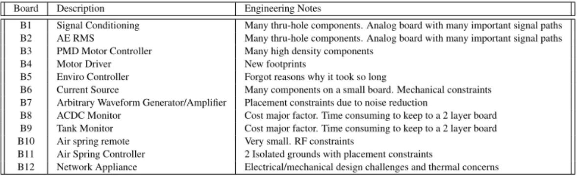
Board Description Engineering Notes

B1 Signal Conditioning Many thru-hole components. Analog board with many important signal paths

B2 AE RMS Many thru-hole components. Analog board with many important signal paths

B3 PMD Motor Controller Many high density components

B4 Motor Driver New footprints

B5 Enviro Controller Forgot reasons why it took so long

B6 Current Source Many components on a small board. Mechanical constraints

B7 Arbitrary Waveform Generator/Amplifier Placement constraints due to noise reduction

B8 ACDC Monitor Cost major factor. Time consuming to keep to a 2 layer board

B9 Tank Monitor Cost major factor. Time consuming to keep to a 2 layer board

B10 Air spring remote Very small. RF constraints

B11 Air Spring Controller 2 Isolated grounds with placement constraints

B12 Network Appliance Electrical/mechanical design challenges and thermal concerns

Table 2:Description of boards analyzed.

capture component and pin density, we define them with equa-tion 2 and equaequa-tion 3 respectively.

Component Density₌ # Components

PCB Area×# Sides w/ components (2)

Pin Density=

# Pins

(PCB Area) (3)

Table 2 gives a description of the boards along with the en-gineering notes that we were able to gather from the designers. Boards B7-B12 used SPECCTRA for OrCAD which is a com-mon auto-router used in industry. No data was available on the use of an automatic router for the other boards but it can be safely assumed that some auto-route tool was used.

Board Statistic Description

PCB Size (mm2_{) Physical size of the PCB}

# of Sides w/ Comp Either 1 or 2 sides has components

# of Routing Layers Layers used for routing traces

# of Layers The total number of layers in the PCB

Components

# Passive Passive components (resistors. . . )

# Digital Digital integrated circuits (IC)

# Analog Analog ICs or devices (opamps. . . )

Total # Total count of all components on PCB

Total Area (mm2_{) Total area of all components on PCB}

Density Ratio of component area to area

Pins

# Passive Pins for all passive components

# Digital Pins for all digital components

# Analog Pins for all analog components

Total Pins for all devices on PCB

Density Ratio of number of pins to area

Table 3:Description of the statistics gathered from the PCBs.

In discussions with the designer of boards B8 and B9 the size of the LCD in the system dictated the size of the PCB and the housing that contained it. The LCD was counted as a component in our analysis and took one complete side of both of these boards, forcing the placement and routing of all other components to one side. Cost was the main consideration for both these boards also and this forced the designer to route everything using only 2 layers.

Among boards B7 through B11 the smallest board, B10,

was judged to be the most difficult to layout, whereas boards B7 and B11 were the easiest. This was attributed to the areas available to do the placement and routing. B7 and B11 were two of the largest boards reviewed and they were not area con-strained, this gives much latitude to the designer for placement and makes the autorouter produce better results. With a more constrained area more human intervention is required during the routing phase which was the case for B10.

Board B12 had the longest system development time which extended the layout time due to the many system changes. At times in a PCB design there exist situations in which the PCB designer can not make forward progress due to electrical and mechanical design choices and issues, hence idle times. For this particular project it actually took approximately 5 months to resolve all issues (which were not related to PCB design ef-fort, for example, cosmetic, placement of I/O). The actual lay-out time is estimated to be ablay-out 10 weeks but would be shorter if starting from a complete (and unchanging) specification.

For the placement stage we only had to consider the num-ber of sides of the board on which components were mounted. Most of the boards in this study had the components all on one side, though a few had bypass capacitors mounted on one side, which accounted for a negligible amount of space. Again, thru-hole devices would affect the available placement area as it did the available routing area as space would be lost on both sides of the board, unlike with surface mounted components. This was not a factor in this study since most boards only used one side for placement. Boards B8 and B9 had components on both sides but one side was populated by only one component, the LCD. Board B10, the only other board with components on both sides, did not have any thru-hole devices present.

5

Evaluation

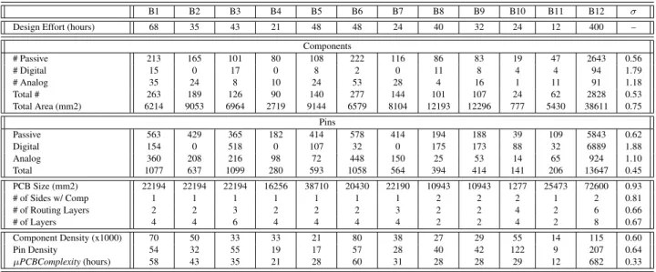
Our evaluation analyzes 12 different printed circuit boards from two seperate companies. Table 4 shows the main results and characteristics for each of these. The first column corre-sponds to each of the statistics or metrics presented in Table 3 (Section 4). Columns B1 to B12 correspond to each of the boards (Table 2). The last column corresponds to the σ be-tween the row and design effort. Since the boards either were designed by the same team, or we only had one board from a

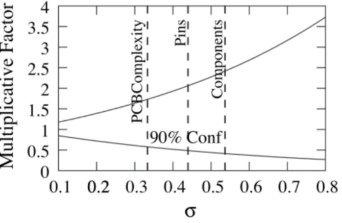
particular company, we do not evaluate the productivity factor (ρ). This simplifies the analysis, and we can use non-linear regression instead of the mixed-effects non-linear regression model. Withσwe can compute the confidence interval. For the lognormal distribution used, the mapping betweenσ and the 90% confidence interval is shown in Figure 1. We will use this chart to compare the accuracy of different estimators.

0.8

0.5

1

1.5

2

2.5

3

3.5

4

0.1 0.2 0.3 0.4 0.5 0.6 0.7

0

0.2

Multipli

cative Facto

r

σ

90% Conf

Figure 1:Mapping between the standard deviation of the error (σ) and the 90% confidence interval for the lognormal error distribution used.

The design effort values were obtained by interviewing the original designers. Obviously, there is perfect correlation with itself soσ= 0. A zeroσresults in a perfect(1,1)confidence interval. We now proceed to analyze easily available statis-tics like number of components and pin count. These two sets of statistics are easily available before the PCB design starts. They are part of the PCB specification.

From the boards analyzed, we observe that it is best to use the total number of components to estimate design effort (σ= 0.53). Although traces for analog components and digital components are more difficult than traces for passive compo-nents, the low amount of digital and/or analog components on several of the boards make it difficult to use them as a method to estimate effort. Figure 1 shows the confidence interval for aσ = 0.53as the intersection between the components line and the confidence interval line(0.41,2.39). This means that using the number of components on the specification, we have a 90% confidence that the design effort would be between 0.41 and 2.39 times the prediction.

Statistics about the pins are as easily available as compo-nents even before the design starts. The number of pins is a better predictor (σ = 0.45) than the number of components. The resulting 90% confidence interval for the number of pins is(0.47,2.09). This means that just by using the pins, we have a 90% confidence that the prediction is around half or double the expected design effort. Not shown in the table is the result of combining the number of pins and the components to pre-dict design effort. The results did not improve because there is a high correlation between pins and components.

Area is not such an effective metric. Even assuming a

per-fect knowledge if the final dimension of the board, we can just estimate design effort with a(0.21,4.61)confidence interval. Table 4 also shows other statistics such as number of sides used, routing layers, and number of layers. Those statistics are not so useful by themselves because they are highly quantized, and this makes them difficult to use to predict effort.

The proposedµPCBComplexitymetrics are now evaluated. To obtain µPCBComplexity shown in Table 4, we analyzed multiple combinations of parameters and followed sugges-tions from experienced board designers. The best results were achieved when using the following equation:

Effort∝# Passive Comp.+Comp. Density+Pin Density (4) Section 4 explains how to compute component density and pin density. To obtain the factors on equation 4, we perform non-linear regression as explained in Section 3. Although neither pin nor component density can achieve better predic-tions than the number of pins, when integrated together in the µPCBComplexity metric we achieve a 0.33 σ. As Figure 1 shows, this represents a(0.58,1.72)confidence interval. This roughly means that by using the proposed µPCBComplexity

metrics, with a 90% confidence designers can predict design effort with less than 40% error.

Figure 2 shows a scatter-gather plot between design effort and ourµPCBComplexitymetric. Each point corresponds to a different board. The plot does not include the B12 board to zoom on the area where most of the boards are located. This plot is an intuitive way to see that there is a high correlation between design effort and the metric proposed.

0 20 40 60 80 100 0 20 40 60 80 100 uPCBComplexity Design Effort

Figure 2: Scatter-gather plot of design effort vs. PCB metric

complex-B1 B2 B3 B4 B5 B6 B7 B8 B9 B10 B11 B12 σ

Design Effort (hours) 68 35 43 21 48 48 24 40 32 24 12 400 –

Components # Passive 213 165 101 80 108 222 116 86 83 19 47 2643 0.56 # Digital 15 0 17 0 8 2 0 11 8 4 4 94 1.79 # Analog 35 24 8 10 24 53 28 4 16 1 11 91 1.18 Total # 263 189 126 90 140 277 144 101 107 24 62 2828 0.53 Total Area (mm2) 6214 9053 6964 2719 9144 6579 8104 12193 12296 777 5430 38611 0.75 Pins Passive 563 429 365 182 414 578 414 194 188 39 109 5843 0.62 Digital 154 0 518 0 107 32 0 175 173 88 32 6889 1.88 Analog 360 208 216 98 72 448 150 25 53 14 65 924 1.10 Total 1077 637 1099 280 593 1058 564 394 414 141 206 13647 0.45 PCB Size (mm2) 22194 22194 22194 16256 38710 20430 22190 10943 10943 1277 25473 72600 0.93 # of Sides w/ Comp 1 1 1 1 1 1 1 2 2 2 1 2 0.81 # of Routing Layers 2 2 3 2 2 2 3 2 2 4 2 6 0.66 # of Layers 4 4 6 4 4 4 4 2 2 4 2 8 0.67 Component Density (x1000) 70 50 33 33 21 80 38 27 29 55 14 115 0.60 Pin Density 54 32 55 19 17 57 28 40 42 122 9 207 0.64 µPCBComplexity(hours) 58 43 35 21 28 60 31 28 28 29 12 682 0.33

Table 4:Statistics, design effort, and correlation results of study boards.

ity increases as the component and pin density increases. De-signers can increase the number of layers on the PCB to de-crease the pin density or inde-crease the area to reduce both den-sities. The problem is that both approaches require more costly boards. As a result, designers trade off between time to market and density.

6

Conclusions & Future Work

The goal of this paper is to introduce an initial exploration of the correlation between some easily obtained metrics from the design of a PCB, and the design effort required during the lay-out stage of development. To do so we extend a previously proposed complexity model [1] to the PCB domain. Furhter, many simplifications have been made; we do not account for traces of differing sizes, we ignore hole sizes or density, the frequency of the boards are also not considered, nor the extra considerations required for analog noise filtering. Also, addi-tional PCBs from more companies with teams of differing sizes may be needed in order to develop a more general model for a general prediction of design effort.

Many factors and constraints affect the design effort re-quired for a board to be successfully placed and routed. Some difficulty metric would be helpful but guidelines need to be es-tablished as “difficulty” is a fairly subjective term. Being able to analyze different options for a board would be useful, such as being able to change the size of the board to see what effect it would have on the estimated design effort. This can be ex-panded to also include the number of layers since this would ease routing congestion.

The evaluation shows that a simple statistics like PCB area size and number of components yield some correlation with design effort. With a 90% confidence, pins has a (0.47, 2.09) confidence interval. This means that roughly by looking at the number of pins, the typical design time error is half/double with a 90% confidence. Much better results can be achieved

with the proposed µPCBComplexitymetric. In that case the confidence interval for a 90% confidence is (0.58, 1.72). This roughly means that less than 40% estimation error is done with a 90% confidence.

Despite the good initial results, we believe that much work needs to be done in gathering relevant design metrics in order to evaluate (with associated known design times) and to refine relevant metrics and models for the design effort of modern PCBs. A major goal to our work is to define a set of equa-tions, that given some easily obtainable design parameters, can generate an accurate estimators for design time.

REFERENCES

[1] C. Bazeghi, F. Mesa-Martinez, and J. Renau.µComplexity: Estimating

Processor Design Effort. InInternational Symposium on Microarchitec-ture, Nov 2005.

[2] M. Chincholkar and J. Herrmann. Modeling the impact of embedding passives on manufacturing system performance. September 2002. [3] E.L. Crow and K. Shimizu. Lognormal Distributions: Theory and

Ap-plication. Dekker, 1988.

[4] T. DeMarco and T. Lister. Peopleware Productive Projects and Teams. Dorset House Publishing, 1999.

[5] JR. Frederick P. Brooks. The Mythical Man-Month. Addison-Wesley, 1995.

[6] A. B. Kahng. Design technology productivity in the dsm era (invited talk). InConference on Asia South Pacific Design Automation, pages 443–448. ACM Press, 2001.

[7] B.S. Landman and R.L. Russo. On a pin versus block relationship for partitions of logic graphs. IEEE Transactions on Comput., (12):1469– 1479, Dec 1971.

[8] L. H. Putnam and W. Myers.Five Core Metrics: The Intelligence Behind Successful Software Management. Dorset House Publishing, May 2003. [9] Numetrics Management Systems. Design Complexity and Productiv-ity. Technical report, Numetrics Management Systems, Inc., 2004. http://www.numetrics.com.

[10] The R Development Core Team.The R Reference Manual - Base Pack-age. Network Theory Limited, 2005.