Size of the government spending multiplier in the recent financial crisis

(1)

Size of the Government Spending Multiplier in the

Recent Financial Crisis

Economics Master's thesis Anna Louhelainen 2011 Department of Economics Aalto University School of Economics

(2)

SIZE OF THE GOVERNMENT SPENDING

MULTIPLIER IN THE RECENT FINANCIAL

CRISIS

Master’s thesis

Anna Louhelainen

25.1.2011

Economics

Approved by the Head of the Economics Department ______ and awarded the grade _______________________________________________________________________

(3)

AALTO UNIVERSITY SCHOOL OF ECONOMICS ABSTRACT

Master’s Thesis in Economics 25.1.2011 Anna Louhelainen

SIZE OF THE GOVERNMENT SPENDING MULTIPLIER IN THE RECENT FINANCIAL CRISIS

In this thesis I study the size of the fiscal multiplier in the economic conditions of the recent financial crisis. The objective is to find out how large the fiscal multiplier can be expected to be in the 2008 crisis and what are the main factors affecting its size. The thesis is conducted in the form of a literature review, where I base my analysis on previous studies and relevant theory.

Throughout the thesis I follow a New Keynesian perspective assuming some degree of price and wage stickiness. The assumption is essential for achieving higher multipliers and is widely used in academic literature on fiscal stimulus.

I find that in a financial crisis with zero interest rates, fiscal multipliers can be clearly higher than during normal times. Provided that the stimulus measures meet certain requirements, the multiplier can reach values greater than 1. These requirements state that stimulus needs to be purely temporary and accompanied by accommodative monetary policy, and higher fiscal spending should be followed by spending cuts in the future. Fiscal measures should preferably not be subject to considerable implementation lags and the stimulus period should last precisely as long as the financial distress continues. The announcement of upcoming stimulus measures has to be credible.

The 2008 crisis and the Great Depression share similarities, the most important ones being the magnitude and global nature of the crises. Fiscal policy could have contributed more to the recovery from the Great Depression had it been used more extensively, and the resulting multipliers could have been larger too. Therefore, the multipliers for the current recovery

period could be higher than in the 1930s and fiscal policy’s contribution might be more significant in the recent crisis.

Keywords: fiscal stimulus, New Keynesian, zero interest rates, Ricardian equivalence, the Great Depression

(4)

1 Introduction

The world economy is recovering from a crisis that has been described as the worst since the Great Depression of the 1930s. After striking the financial sector it moved on to affecting the real economy by lowering GDP and increasing unemployment rates. As a response, several countries adopted fiscal packages of varying sizes, the U.S. having the largest of all OECD countries (OECD 2009). What is not necessarily so clear, though, is the effect of fiscal stimulus on GDP, and it remains uncertain if fiscal stimulus in reality is such a wise response to the crisis as some policymakers argue. Despite the amount of academic discussion concerning fiscal policy, there is little if any agreement among economists on its effectiveness. For instance, while most would agree that an exogenous increase in money supply will lead to an increase in prices at some point in time, economists can and do disagree even on the sign of the response of private consumption to an exogenous increase in government purchases. Also, by the time a change in fiscal policy has been decided, implemented and takes effect, the cyclical economic conditions might have changed radically and the changes might start working against the recovery. Even so, politically fiscal stimulus has very often been a popular way of trying to boost the economy. (Perotti 2002) Besides being concerned about the efficiency of fiscal stimulus, economists and analysts have been increasingly worried about the state of public finances in the U.S. and several European countries. A large stimulus package can easily lead to a high level of government debt, which can have quite severe and long-lasting consequences when it comes to output and economic growth.

(7)

2

1.1 Previous Research

Since the 1930s and the ideas of John Maynard Keynes on fiscal policy, fiscal stimulus and its effects have been a popular topic of debate among economists. Although during the past few decades there has been notable convergence of views in macroeconomics with some fundamental issues, this is not the case when it comes to fiscal policy (Woodford 2009). In fact, surprisingly little is known about the effects of fiscal policy as many more resources have been devoted to studying monetary policy. The advanced DSGE1 models developed during the past decade (e.g. Smets and Wouters 2003) are continuously used by central banks worldwide to assess the effects of monetary policy but surprisingly few of them have been used for fiscal policy purposes (Hall 2009).

One reason why relatively little empirical work has been done on the effects of fiscal policy is probably the difficulty of obtaining all the data needed, especially over sufficiently long periods of time. The vast majority of the studies have been done using U.S. data (e.g. Blanchard and Perotti 2002, Hall 2009) the reason being simply that there is not enough data on other OECD countries from the 1930s onwards. A few exceptions can be mentioned here, such as Cwik and Wieland (2009), who assess the stimulus programs announced by Euro area governments in 2008 using five different models all estimated with euro area data and Perotti (2002), who has estimated the effects of fiscal policy measures using a structural vector autoregression (VAR) model for five OECD countries, one of them being the U.S. The Great Depression of the 1930s and the effectiveness of fiscal policy measures taken then has been studied quite extensively (e.g. Romer 1992), mostly using U.S. data for reasons mentioned above. Many of these studies have been done by using variations in defense spending, that is, the part of government spending associated with buildups and aftermaths of wars, as a proxy for total government spending (e.g. Almunia et al. 2009, Barro and Redlick 2009). The main reason for this is that changes

1

DSGE refers to a Dynamic Stochastic General Equilibrium model and will be explained in more detail in chapter 3.1.

(8)

3

in defense spending are more suitable for empirical purposes since they can often be treated as purely exogenous shocks. On the contrary, changes in total government spending, which includes also non-defense spending, are typically endogenous, at least to some extent, and are not completely determined by factors outside the model. However, using defense spending can incur some additional problems that will be discussed in more detail in chapter 7.

Lately the trend in macroeconomic research has been the use of VAR models, since they allow including more variables in the analysis than simple regression models. For example Blanchard and Perotti (2002) and Perotti (2002) have studied fiscal policy effects using a VAR approach. Apart from the modern and complex VAR methods, a theoretical analysis on a more general level using structural models has been done by some authors. Structural models also serve better for identifying information and differentiating between separate fiscal instruments (Coenen et al. 2010). For instance Christiano et al. (2009), Eggertsson (2009) and Woodford (2010) all use a structural model to study the effects of fiscal policy under differing assumptions about monetary policy and interest rates. Whatever the model in use, it should be chosen so that it corresponds to a crisis-like environment; in particular, one should be extremely cautious when applying estimations made under normal business cycle conditions to financial crises.

1.2 Research Question and Method

In this thesis I will study the effect that an increase in government purchases has on GDP in the economic conditions of the latest crisis. This can as well be interpreted as finding out whether fiscal stimulus is effective in helping the economy to recover from a recession or not. I attempt to do this by studying the size of what has been known since Keynes as the fiscal or government spending multiplier, that is, the proportional change in GDP when public expenditure is increased by a certain amount. My research question will be as follows: How large (or small) is the fiscal

(9)

4

multiplier in the recent crisis and under which conditions can the multiplier be expected to be large? I will try to identify the most important factors affecting the size of the multiplier and explain the mechanisms through which they operate, focusing on the special conditions created by the crisis. I will restrict my analysis to government spending on goods and services so my concern will be with government

purchases, not all of government spending, which would also include taxes and other transfers.

The research will be conducted in the form of a literature review and I will go through some relevant theory behind fiscal stimulus as well as present results from previous studies. I will discuss the effects of monetary policy, duration and financing of the stimulus. What I will use as a reference and a comparison with the recent crisis is the Great Depression of the 1930s, namely I will study what the two crises have in common and try to apply the results from the Great Depression to the 2008 crisis. I shall start with a brief overview of the characteristics and magnitude of the recent crisis, which will be followed by a comparison with the Great Depression. The idea is to find out whether the two crises have enough in common to be compared with each other and whether or not the results from the Great Depression can be applied to the current situation.

In the third chapter I will present the theoretical framework for fiscal stimulus. I will discuss the differences between the two most frequently used theories, Neoclassical and New Keynesian, and take a look at the differences in their views concerning the effects of fiscal stimulus. I will concentrate more here on New Keynesian theory, as it is more commonly used for studying fiscal policy. I will also mention some challenges that modern macroeconomic models in general are facing and their restrictions. Then I will take a look at zero interest rates and liquidity traps, which are both common in financial crises, and see what effects they have on the size of fiscal multipliers. Last, I will briefly go through findings on the multiplier effects of tax cuts.

In the fourth chapter I will take a look at the size of fiscal multipliers under three alternative assumptions about monetary policy and interest rates. I will move on from the simplest case of a constant real interest rate to first consider a policy where

(10)

5

nominal interest rates are set according to the Taylor rule and then the case of constant nominal interest rates. The last scenario is particularly interesting for the analysis of this thesis, as the assumption of a constant nominal interest rate applies to the case of zero interest rates, which in turn is closely related to the conditions of the recent crisis.

In the fifth chapter I will study the optimal timing and duration of an effective stimulus package. First I will explain what factors determine how long the stimulus period should last. Then I will see what happens to the short-term multiplier if the stimulus measures become permanent, and discuss the long-term crowding-out effects resulting from a high level of public debt. Finally I will consider the role of implementation lags and anticipation.

In the sixth chapter I will discuss topics related to government debt. I first consider the Ricardian equivalence theorem and its implications, which will be followed by more realistic cases that allow for the existence of non-Ricardian households alongside with Ricardian households. I will also take a look at the possibility of financing the stimulus with spending reversals instead of higher taxes and see what an effect changing to this strategy has on the size of the multipliers.

In the last chapter I will take a step back and analyze the recovery from the Great Depression in more detail. I will present some views on the factors that contributed the most to the end of the Great Depression. Since most of the multiplier estimations have been done using defense spending, I will discuss this approach and comment on some issues regarding the use of defense spending in the estimates. Then I will review some fiscal multipliers estimated from the recovery period after the Great Depression. Finally I will finish the thesis by presenting the conclusions.

(11)

6

2 Overview of the Crisis

The world is recovering from its worst economic crisis in several decades. What started mainly as a housing sector crisis and deepened into a severe credit crunch has become a real economy crisis with increasing unemployment and substantial decreases in production. The deterioration of public finances is notable not only in advanced economies but also in developing countries and the world as a whole (IMF 2009a).

According to OECD (2009) virtually all OECD countries have taken measures in supporting the economy with fiscal stimulus packages, the U.S. having the largest fiscal package of 5,6 % of 2008 GDP and four other OECD countries amounting to fiscal packages of 4 % or more of 2008 GDP.2 However, empirically there is mixed evidence about the effectiveness of fiscal stimulus in stimulating the recovery.

One of the characteristics that are distinctive compared to previous crises and that sets challenges for the policymakers is the collapse of the financial system and liquidity, and the financial nature of the crisis can weaken the response to traditional monetary expansion. In addition, some countries might have already used monetary expansion, which limits the central bank’s room to lower interest rates. In such a

situation, the role of monetary policy should be more in supporting fiscal stimulus by avoiding increases in interest rates until output begins to recover. (IMF 2008)

2.1 Background and Special Characteristics

In the first three quarters of 2008, the following year after the U.S. subprime crisis in August 2007, economic activity in advanced countries slowed down but did not yet collapse, while developing economies still continued to grow. It was not until

2

Sizes of the fiscal packages are measured by the cumulative impacts on fiscal balances over the period 2008- 2010.

(12)

7

September 2008 and the default of the U.S. investment bank Lehman Brothers when the situation started to deteriorate rapidly and overall confidence and liquidity were practically lost in the financial markets. Banks experienced large write-downs and tightened their lending standards. Financial market distress could be seen in strong demand for liquid assets, increased volatility, falling equity prices and widened spreads for corporate bonds. (IMF 2009a)

By the end of 2008, the credit crunch had already moved on to the real activity as production and international trade collapsed in both advanced and emerging economies, which was followed by increased unemployment. The fact that firms and consumers had little confidence in economic prospects and the credibility of the policy responses magnified the reactions and the scale of the problems. Even though towards the end of the crisis policy responses have been more efficient in fighting financial market problems, conditions on the financial markets have remained highly stressed. (IMF 2009a)

What makes this crisis distinct from some previous, severe crises is first its overall impact on the world economy: in 2009 the world economy as a whole experienced its first contraction since the Second World War, as the world GDP fell by 2,0 % (UN 2010). As opposed to some other, more regional crises, the recent crisis has had an impact on almost every country in the world. Also, the fact that the U.S. was the epicenter and actually the starting point of the crisis is worth mentioning, since this is the case for the first time after the Great Depression. The global aspect also means that any export-led recovery strategy does not work in stimulating the economy (IMF 2008).

Also the scale of the financial system problems is exceptional, since the liquidity in the financial markets was at some point almost completely lost (e.g. IMF 2009b). Because of this, policy measures taken should be focused not only on stimulating aggregate demand and employment and restoring confidence but also on repairing the financial system failures (IMF 2008).

(13)

8

2.2 Comparison with the Great Depression

The 2008 crisis has been widely compared to the Great Depression of the 1930s, mainly because of the magnitude and global aspect that distinguish them from other severe crises. Also, both crises have the U.S. economy as the center of the crisis, while many other important crises have developed in smaller, often emerging economies (Helbling 2009). Globally the fall in output in the recent crisis is comparable to that of the 1930s, even though for example in the U.S. the output collapse was greater during the Great Depression (Almunia et al. 2009).

As opposed to today, in the 1930s production was concentrated mainly in the U.S. and Europe, which created a strong distinction between the industrialized products of the north and the primary products of the south. Since it was mainly industrialized production that collapsed during the recession, the production collapse was a concern in the industrialized countries, while the production in Asian and Latin American developing countries remained more stable. On the contrary, today the industry is spread around the whole world and the output fell rapidly everywhere during the first year of the crisis. (Almunia et al. 2009)

In the 1930s, regardless of the more stable production in developing countries, commodity prices fell more sharply there than in industrialized countries. This was due to the fact that international trade in manufactured goods fell more sharply than for primary goods, which resulted in relatively lower prices for primary goods and made the developing countries worse off regardless of a more stable level of production. This worked as a key mechanism in lowering incomes in the countries of the south. As a consequence, the developing countries were also badly affected and the nature of the crisis was strongly global, as in the recent crisis. (Almunia et al. 2009)

During the recent crisis, trade fell much more rapidly than in the 1930s, which implies a greater elasticity of trade with respect to production (Almunia et al. 2009). This could be attributed to the global fragmentation of production or, as Tanaka (2009) refers to it, vertical specialization, which means that manufacturing firms are

(14)

9

increasingly specializing in certain stages of the production process. This also means that a product can cross national borders several times before reaching its final consumer. If production is more fragmented globally, then trade flows respond more sharply to changes in global demand.

Almunia et al. (2009) argue that while the growth of vertical specialization can explain the absolute decline of trade, it remains unable to explain the percentage

decline or greater elasticity of trade with respect to production. They therefore refer to another explanation, which is the changing composition of trade: since it was output and trade of manufactured goods that collapsed in the 1930s and since the proportion of manufactured goods in the world trade has risen from 44 % in 1929 to 70 % in 20073, the decrease in world trade was undoubtedly greater in the 2008 crisis. If manufacturing had been as important a share of world trade as it is today, total world trade would have fallen at a rate comparable to the current situation. In the recent crisis interest rates were cut down more rapidly and from a lower initial level than in the 1930s, the Bank of England and the Fed having both reacted faster than the ECB. Monetary expansion has also been more rapid now than during the Great Depression. In addition, it seems that not only advanced economies but also developing countries are using fiscal policy more aggressively as opposed to the 1930s. (Almunia et al. 2009) All in all it looks as if policy measures were taken faster and more aggressively than in the 1930s.

Also, because of different types of exchange rate obligations in the 1930s (e.g. the gold standard), several countries were unable to practice expansionary monetary policy and reluctant to apply fiscal stimulus fearing it could attract more imports and lead to a drain of reserves. Since now all major economies have flexible exchange rates, also the central banks have the possibility to respond aggressively. There are some exceptions, namely countries that are pegging their currency to some other currencies. These commitments can sometimes lead to adverse policy responses or prevent the use of monetary policy in stimulating the economy, since in order to maintain the commitment the central banks may be obliged to, for instance, raise

3

1929 data is available in http://unstats.un.org/unsd/trade/imts/historical_data.htm and 2007 data in http://www.wto.org/english/res_e/statis_e/its2008_e/its08_merch_trade_product_e.htm.

(15)

10

interest rates despite the lower aggregate demand. In general, however, because of the broader use of flexible exchange rates in the recent crisis, the monetary authorities have had more power in fighting the recession than in the 1930s. (Almunia et al. 2009)

Liquidity and funding problems have played a key role in the financial sector transmission in both crises. Concerns about the net worth and solvency of financial intermediaries were at the root of both crises, although the specific mechanics were different, given the financial system’s evolution. In the Great Depression, in the absence of deposit insurance, the problems resulted from the weakening of the deposit base of US banks. In four waves of bank runs, about one third of all US banks failed between 1930 and 1933. The bankruptcy of the Austrian bank Creditanstalt in 1931 finally resulted in bank runs also in European countries. In the recent crisis, the existence of deposit insurance has largely prevented bank runs by the public. Instead, funding problems have been created by financial intermediaries relying on wholesale funding, particularly those issuing or holding, directly or indirectly, U.S. mortgage-related securities whose value was hit by increasing mortgage defaults in 2007. With large international linkages, the problems were immediately global despite their U.S. origins. In contrast, the spillover effects were more gradual in the 1930s, with the U.S. funding problems transmitting through increased capital flows to the U.S. and money supply contraction in the source countries. (Helbling 2009)

During the Great Depression, there was a similar near-zero interest rate type of a situation, with signs of a liquidity trap, as in the 2008 crisis (Almunia et al. 2009). In short this refers to a situation where additional interest rate cuts are no longer possible, because the nominal interest rate has already been cut down close to zero. In the case of a liquidity trap the demand for money becomes infinitely elastic, so expansive monetary policy is not useful in stimulating consumption either. In conditions like these, fiscal policy is often viewed as a good way of stimulating the economy, since traditional monetary policy cannot be used and crowding out of private investment becomes less likely with interest rates close to zero. It has also

(16)

11

been argued that the reason why fiscal policy did not work well in stimulating the recovery in the 1930s was that it was hardly used (Almunia et al. 2009).

In conclusion, the recent crisis is similar enough to be compared with and, to some extent, analyzed based on the Great Depression. What the two crises have in common is the already mentioned global magnitude and rapid decline in trade of manufactured goods as well as financial sector distress. It seems as if policy measures to recover from the crisis had been taken more quickly in the recent crisis, which may also be due to the fact that it has been easier to do so.

3 Basic Facts about Fiscal Stimulus

In this chapter I review some general facts and findings on shocks to government spending and their effects on output. I will present some relevant theory and go through previous literature in order to find theoretical support for fiscal stimulus. I will then discuss other topics related to fiscal stimulus, mainly restrictions and special conditions that a crisis situation creates on the use of monetary policy. Finally I will briefly consider the effects of tax cuts on output and compare them with those of increased government purchases.

3.1 Theoretical Framework

3.1.1 Different Theories

The traditional Keynesian theory suggesting high fiscal multipliers is nowadays quite unanimously regarded as an insufficient tool in analyzing the economic environment. Traditional Keynesian models that aim to explain the short-run effects of alternative

(17)

12

government policies fall short in one important aspect: they do not include forward-looking consumers and their preferences or firm objectives in their preliminary assumptions.

On the contrary, Neoclassical models explain the macroeconomic environment by building on micro foundations and assume rational, utility-maximizing consumers and profit-maximizing firms that make their decisions based on full and perfect information. Neoclassical models assume prices and wages to be fully flexible and do not include market rigidities in their general framework. Lately the Neoclassical theory has been increasingly merged with modern Real Business Cycle (RBC) theory that builds macroeconomic models for quantitative analysis using optimizing behavior at the individual level. Neoclassical RBC models assume fully flexible prices and wages and study the effects that real economic shocks have on business cycle fluctuations.

Since in the real world there are always some market frictions, it is quite optimistic to assume perfect information and fully flexible prices. New Keynesian models try to approach this problem by allowing for market frictions, namely sticky prices and wages, as in the Old Keynesian theory, but adding the microeconomic aspect and forward-looking, utility-maximizing consumers in their framework. They use traditional, Old Keynesian theory as a basis and attempt to provide micro foundations for key Keynesian concepts. More recently New Keynesian theory has been greatly influenced by RBC theory and by combining the theoretical basis of RBC models with traditional Keynesian ingredients, New Keynesian models provide a framework that has become the basis of a new generation of models used increasingly for analysis and forecasting purposes (Galí 2008).

New Keynesian models have adopted many of the tools originally associated with RBC theory, such as the use of Dynamic Stochastic General Equilibrium (DSGE) models that are based on optimizing consumer and firm behavior and rational expectations. One of the more general characteristics of the New Keynesian framework is its flexibility when it comes to accommodating to different extensions made to the basic model. (Galí 2008) As opposed to the classical Keynesian view,

(18)

13

New Keynesian theory assumes consumers to be forward-looking and rational and firms to be profit-maximizing and is in that sense a lot more similar to the Neoclassical view than the Old Keynesian theory.

As always when it comes to economics, there is disagreement on whether New Keynesian theories are adequate for evaluating the effects of economic policies. New Keynesian models have been used widely in estimating the effects of monetary policy (e.g. Smets and Wouters 2003, Christiano et al. 2005), but not as extensively when it comes to fiscal policy. Indeed, in attempts to estimate the government expenditure multiplier empirically the results vary drastically depending on the initial assumptions made as well as the type of model used.

Also, few macro models of any kind involve a monetary sector. In the majority of these models households choose the optimal level of consumption according to the life-cycle-permanent-income principle and depending on their intertemporal budget constraint. In turn, firms choose inputs to maximize profit, subject to wage and capital rental. On the contrary, monetary sector is not formally modeled, but instead, consistent with modern central bank practice, the economy is supposed to have a Taylor rule relating the interest rate to the rate of inflation. In addition, recently one more problem has been recognized when it comes to modern general-equilibrium macro models: they miss important features of financial markets, especially the widened spreads between safe government interest rates and private rates, which have occurred in the recent crisis, for example. (Hall 2009)

3.1.2 Suggestions of the Different Theories

The reason why Old Keynesian models yield such high multipliers lies in their non-dynamic nature: since they assume consumers make their consumption decisions based solely on current disposable income instead of taking into account the present value of future disposable income, there is no crowding out effect of private consumption. Consumers do not anticipate the decrease in future income caused by

(19)

14

the government’s need to finance the higher level of expenditure and they consume

all the additional income they get. An analogous interpretation goes for the private sector firms as well.

As soon as the assumption of forward-looking consumers and firms and maximization of life-cycle utility is added into the model, the situation changes quite dramatically. When the government increases expenditure, the private sector anticipates that the spending needs to be financed with higher taxes at some point in the future or with a higher level of debt, which would in turn result in higher interest rates, and they save some fraction of the additional income. This is the reason why in practically all the modern empirical and theoretical studies there is crowding out of private consumption to some extent when public spending is increased. Empirically, New Keynesian models yield considerably lower multipliers than Old Keynesian models (see e.g. Cogan et al. 2009). It is worth mentioning, though, that even when consumers are forward-looking, the fraction of consumption entering into the life-cycle consumption theory is not 100 %, since there is always a part of consumers who would be willing to borrow and to smooth their consumption, but are not able to do so and are constrained to spending their current income. (Hall 2009)

The assumption of rational expectations and intertemporal optimization is what the New Keynesian and Neoclassical models have in common. Where they differ is the interpretation of price and wage flexibility. In purely neoclassical models full employment follows implicitly from the assumption of perfectly flexible prices and wages. Therefore increases in government purchases crowd out private investment and consumption and do not raise output substantially. The output multiplier, which is the effect of increased government purchases on aggregate output is only slightly positive and the consumption multiplier clearly negative. The reason is that even with full employment, an increase in output and aggregate demand can only come from increased employment. With no employment reserves available, any increase in employment must necessarily drive the wage down, which in turn will result in less labor supply. The attempt to stimulate aggregate demand by any means that raises product demand and consequently employment and output must decrease consumption, contrary to common sense. (Hall 2009)

(20)

15

Woodford (2010) finds, quite consistently with the reasoning above, that in the case of Neoclassical theory with perfect competition the multiplier is always positive but necessarily less than one which means private expenditure is crowded out to some extent. The higher the degree of intertemporal substitutability and the more sharply rising the marginal cost of employing additional resources in production, the smaller the multiplier. If there is monopolistic competition on the market, it follows that if there is any delay in the adjustment of prices and wages, the multiplier can be slightly larger than with perfect competition.

According to Hall (2009), the two main ways of obtaining higher multipliers are related to (1) the margin of price over cost, or the markup ratio, and (2) the elasticity of labor supply. If the markup ratio is not constant but falls during expansions, the markup declines as output increases and prices stay constant during a boom that increases production costs. This can also be expressed as price stickiness, one of the main assumptions behind New Keynesian models. During an expansion, the declining markup allows for the wage to rise or at least not to fall as much as it would in the case of a constant markup. In this sense, it allows households to supply much more labor when the government increases expenditure than in the case of fully flexible wages. Elastic labor supply can in turn be associated with sticky wages. However, in an economy with sticky wages and without sticky prices, the government spending multiplier is always negative, that is, in order to obtain high multipliers, both of the conditions expressed above need to hold.

3.2 Liquidity Trap and the Zero Interest-rate Lower Bound

A situation where government spending multipliers are both theoretically and empirically higher than usual is when the nominal interest rate is restricted by a zero lower bound. This refers to a situation where it is impossible for the central bank to stimulate aggregate demand by lowering short-term nominal interest rates, since they cannot be lowered below zero, or some other small lower bound. This in turn

(21)

16

leads to a situation, where the real interest rate is higher than it should be for the economy to be able to recover. The zero interest-rate lower bound is typically accompanied with a liquidity trap, where attempts to increase liquidity in the market by supplying more money are useless, since all the additional liquidity is absorbed and it does not affect the level of interest rates or economic activity (Benigno 2009). The liquidity trap and zero lower bound on interest rates also imply that conventional monetary policy in the form of lowering interest rates is no longer effective when it comes to stimulating aggregate demand, which has sometimes been used as a factor supporting the use of fiscal stimulus. Also, in earlier studies it has been found that fiscal multipliers are higher and fiscal policy is more effective if it is carried on when the zero lower bound binds. (e.g. Christiano et al. 2009) In a normal situation, if public demand is increased, it will lead to a rise in interest rates, which will result in crowding out of private investment. With the zero lower bound this need not be the case, that is, the real interest rate and the nominal interest rate do not need to rise in response to fiscal stimulus. Since the increase in government spending is often associated with higher inflation expectations, the real interest rate can actually decrease as a result of fiscal stimulus. Government purchases should thus be expected to have an especially strong effect on aggregate output if the zero interest-rate lower bound is binding. (Woodford 2010) Accordingly, Christiano et al. (2009) find that the multiplier is a lot larger if the nominal interest rate does not rise in response to increased government spending and they find multipliers as high as 2 if the nominal interest rate remains constant while government spending goes up for eight quarters.

There is also another view on the effectiveness of monetary policy in a liquidity trap, pointed out by Krugman (1998) and also discussed in Benigno (2009), which does not see monetary policy as completely ineffective. Since in a liquidity trap, lowering the real interest rate creates expectations for future inflation, it can offer a solution when more conventional monetary policy does not work. Since people anticipate the price level to be higher in the future, the real interest rate will decrease based solely on expectations of higher prices. It is worth pointing out, though, that in practice it may be hard for the central bank to commit to future inflation (Christiano et al.

(22)

17

2009). A liquidity trap is always the product of a credibility problem where the public believes that the monetary expansion will not be sustained. Without the ability to carry on credible monetary policy it seems logical that committing to high inflation in the future is not too credible either. For structural reasons inflationary expectations can sometimes be necessary but that should never imply that credibly sustained monetary expansion is ineffective. (Krugman 1998)

Eggertsson (2009) has also studied the effectiveness of different fiscal policy measures when the short-term nominal interest rate has been cut down to zero. Using a standard New Keynesian DSGE model he finds, that the most effective ways are increasing public spending and committing to future inflation. He argues them to work ideally together, since government spending itself creates inflationary expectations and should not suffer from credibility problems in that sense. When the zero bound on interest rates is binding, insufficient demand is the main problem and different policies should mainly focus on increasing aggregate demand instead of tackling with the supply side. When it comes to tax cuts on wages and capital, Eggertsson finds quite surprisingly that they can have contractionary effects on consumption and can induce more saving. However, since tax cuts tend to increase budget deficits, he raises one channel through which tax cuts can be effective in stimulating the economy: by creating inflationary expectations. This and other findings from the effects of tax cuts will be discussed in more detail in the next chapter.

3.3 Multiplier Effects of Tax Cuts

Even though in this thesis I restrict my analysis to public spending on goods and services, for motivationary reasons and in order to have a point of comparison I will briefly review some findings on the multiplier effects of tax cuts as well.

Tax cuts and government spending operate on aggregate demand through different channels: government spending (consumption and investment) affects directly

(23)

18

aggregate demand while tax cuts operate primarily through their effects on the disposable income of the private sector. It is widely accepted in the literature that fiscal measures that have a direct impact on the demand side have larger multipliers than those that operate mainly through affecting the households’ spending behavior.

(Coenen et al. 2010) Indeed, when comparing the effects of different fiscal measures several studies have found that increasing government spending, especially government investments, generates larger multipliers than cutting taxes or increasing transfers (see e.g. Roeger and Veld 2009, Freedman et al. 2010).

Eggertsson (2009) finds, using the DSGE model mentioned in the previous chapter, that tax cuts can deepen a recession under the economic circumstances that characterized the crisis of 2008. His key assumption is that the short-term nominal interest rate has been cut down to zero, so that the economy experiences excess deflation and output contraction. In these circumstances he argues tax cuts on wages and capital to have contractionary effects on output. When labor income taxes are cut, they create deflationary pressures by reducing the marginal costs of firms, which in turn causes the real interest rate to rise. When the nominal interest rate has already been lowered to zero, the central bank is not able to lower the nominal interest rate more in order to stimulate the economy. When it comes to capital taxes, in normal circumstances they would increase investment and have an expansionary effect. However, in the circumstances of the recent crisis the problem is not that the capacity of the economy is inadequate, but rather that the aggregate demand is insufficient. This means that cutting capital taxes gives people the incentive to save instead of spending, which obviously deteriorates the situation. On the contrary, sales tax cuts and investment tax credits Eggertsson finds to be effective, since they stimulate spending and aggregate demand instead of focusing on the supply side. In conclusion, when interest rates are positive tax cuts are expansionary, but as soon as the interest rates are cut to zero, the effect becomes contractionary. As a comparison, while the effect of government spending on output is already positive when the nominal interest rate is above zero, it becomes eight times larger with zero interest rates. Eggertsson also points out that many of the previous results on the effects of fiscal policy may not be directly applicable to the

(24)

19

current situation, since in the samples used interest rates remain positive all the time.

Blanchard and Perotti (2002) study the effects of both government spending and taxes on output using a VAR model and event-based sets of U.S. postwar data. Their results consistently show positive tax shocks to have a negative effect on output, which implies that in their model tax cuts have stimulative effects on output. The size and persistence of the effect depend on the specifications, which include deterministic and stochastic trends as well as different subperiods, such as the Korean War buildup. Positive government spending shocks they find to have a consistent positive effect on output and private consumption, but a negative effect on private investment.

An interesting observation is also that the GDP response to fiscal policy has become substantially weaker during the past 20 years for both tax and government spending multipliers and especially the post-1980s tax multipliers are significantly negative. The decline in the efficiency of fiscal policy might be in part due to the world economy becoming more open. Also, during the past decades major economies have been moving from fixed exchange regimes to flexible exchange rates, which can reduce the power of fiscal policy. When interpreting the results from previous studies it is worth noting that because of lack of availability of European data, the vast majority of studies have been done using U.S. data. Since the U.S. is an outlier in many dimensions, the results may not be representative of the average OECD country. (Perotti 2002)

3.4 Discussion

The more advanced and sophisticated macroeconomic models developed during the last decade have made the analysis of fiscal policy decisions more extensive and more realistic. New Keynesian DSGE models that enable a dynamic analysis are increasingly used in several macroeconomic studies, but to a wider extent when it

(25)

20

comes to monetary policy. What the models are still lacking is a formalization of the monetary sector and very often interest rates and inflation are simply assumed to be related to each other according to the Taylor rule. Also, especially when it comes to analyzing the 2008 crisis, including features of the financial sector would be useful, since the financial sector collapse has played such an important role in the crisis. New Keynesian models consistently yield higher fiscal multipliers than Neoclassical models, and allowing for any market rigidities, such as monopolistic competition, increases the multipliers in Neoclassical models. The New Keynesian assumption of sticky prices and wages is a key factor in obtaining high multipliers. Another important assumption when it comes to observing high multipliers, which can easily be related to the latest crisis, is that the zero lower bound for interest rates binds. When the zero lower bound and liquidity trap-like conditions prevail, nominal interest rates do not have to rise in response to increased public spending and private spending is not substantially crowded out. Fiscal policy is especially effective if the zero nominal interest rate is accompanied by inflation expectations. In turn, private investment is normally crowded out to some extent when government expenditure is increased, even in New Keynesian models. The increasing international trade and capital movements as well as wider use of flexible exchange rates have made the response to fiscal policy weaker during the past decades.

When it comes to tax cuts as a means of fiscal policy, they can be contractionary especially with zero nominal interest rates. When evaluating the results of previous studies on tax cuts one should keep in mind that many of the studies have been done using data with positive interest rates and can therefore yield estimates that are not directly applicable. In brief, it is preferable to concentrate on aggregate demand instead of aggregate supply when conducting fiscal stimulus policies.

(26)

21

4 Interest Rates and Monetary Policy

In this chapter I will study the size of the government spending multiplier under differing assumptions of monetary policy. Consistently with many of the empirical DSGE models, I primarily assume prices and wages to be sticky, so that monetary policy has an effect on real activity and the consequences of an increase in government purchases depend on the monetary policy response. According to the Neoclassical theory this would not be the case since fully flexible prices and wages would adjust to any changes in monetary policy.

4.1 Constant Real Interest Rate Multiplier

As a first step in the analysis concerning multipliers under different monetary policy schemes, a useful benchmark is to assume that the central bank maintains an unchanged path for the real interest rate, regardless of the path of government purchases. It is worth bearing in mind though that under realistic assumptions about monetary policy, the real interest rate may well change. The advantage of this multiplier is that it is easier to calculate and that it remains the same under differing assumptions of price and wage stickiness. (Woodford 2010)

Woodford (2010) uses a New Keynesian model to analyze the size of the multiplier. In his model, variations in the level of government purchases are assumed to be purely temporary and monetary policy brings out a zero rate of inflation in the long run, so that the economy converges to a steady state in which government purchases equal , inflation is equal to zero and output is equal to some constant level . Note that the essential assumption here is that the monetary policy is chosen in such a way that the real interest rate is held constant. The operating target for the nominal

interest rate can be chosen according to the Taylor rule, for instance, where the nominal interest rate is adjusted based on the rate of inflation, but the central bank

(27)

22

may as well choose a path for money supply that is consistent with zero inflation in the long run, or the equilibrium can be implemented in some other way.

The economy consists of a large number of identical, infinite-lived households that seek to maximize

∑

[ ( ) ( )]

(4.1)

where is the quantity consumed in period t, the hours of labor supplied, the utility functions satisfy , , , , and the discount factor satisfies . The output is consumed either by households or by the government, so in equilibrium

(4.2) Optimization by households requires that in equilibrium,

( )

(4.3)

where is the one-period real rate of return. It follows from (4.3) that in the long-run steady state, = for all t. Now it also follows that = for all t, so the representative household must be planning a constant level of consumption, at whatever level is consistent with its intertemporal budget constraint. Convergence to the steady state implies that – for large t, hence in equilibrium

(28)

23

(4.4)

for all t. Now the government spending multiplier ( ) is equal to 1. There is neither crowding out of private expenditure nor any stimulus of additional private expenditure.

Even though the simple result obtained here does not require very specific assumptions about wages or prices and their adjustments, the crucial assumption made here is that it is possible for the central bank to maintain the real interest rate constant regardless of the short-run level of government spending (Woodford 2010).

4.2 Interest Rate Governed by a Taylor Rule

Next I consider a slightly more realistic assumption of monetary policy, where the interest rates are set in accordance with the Taylor rule, that is the nominal interest rate is adjusted according to variations in the inflation rate. As opposed to the previous chapter, the real interest rate is not assumed to stay constant during the fiscal expansion. Nominal interest rates will rise as a response to an increase in government spending, which puts upward pressure on inflation.

Christiano et al. (2009) use a New Keynesian model to analyze the government spending multiplier when interest rates are governed by the Taylor rule. They find that the multiplier is given by:

̂ ̂ ̂ ̂ (4.5)

(29)

24

where , and denote output, government spending and private consumption, respectively, ̂ denotes the percentage deviation of from its non-stochastic steady state value4 and . The equation implies that the multiplier is less than 1 whenever consumption falls in response to an increase in government spending, that is when private consumption is crowded out by increased public spending. The baseline parameter values chosen by the authors imply that the government spending multiplier is 1,05. The result might seem quite surprising, since by intuition some crowding out of private spending should be expected because of the negative wealth effect caused by an increase in government spending5. However, this perspective would neglect two key features of the model, the price rigidity and the complementarity between consumption and leisure in preferences. Since prices are sticky in the model, they stay constant when the demand rises, but at the same time production costs increase resulting in a lower price over marginal cost (the markup). The rise in aggregate demand is followed by a rise in employment. Given the complementarity of consumption and leisure in preferences the marginal utility of consumption rises with the increase in employment. As long as this rise in marginal utility of consumption is large enough, it is possible for private consumption to rise as a result of fiscal expansion, which explains the size of the multiplier calculated with the parameter values.

To further assess the importance of the preference specification the authors recalculate the multiplier using a different specification for preferences, where the marginal utility of consumption is independent of hours worked. Across a wide set of parameters they find that the multiplier is always less than 1 with this preference specification.

Next they calculate for various parameter configurations and analyze the multiplier effects of changes in the parameters. Their first observation is that the

4

The authors use a linear approximation around the non-stochastic steady state of the economy in order to solve for the equilibrium.

5_{In the model Ricardian equivalence holds so that from the perspective of the representative} household, the increase in the present value of government purchases equals the increase in the present value of taxes and they both have a negative wealth effect. Ricardian equivalence and its implications on fiscal stimulus are discussed in chapter 6.1.1.

(30)

25

more the marginal utility of consumption rises with the increase in employment, the higher the multiplier, which seems quite reasonable considering the discussion above. Also, the higher the degree of price stickiness, the larger is the multiplier. The observation of a multiplier growing with more price stickiness reflects the fall in the markup when aggregate demand and marginal cost rise, and the effect is even stronger with more price stickiness. For comparison, if prices are perfectly flexible, the markup is constant and the multiplier less than 1 always.

If the real interest rate rises substantially in response to a rise in output, the multiplier is smaller, which seems clear by intuition, since a rise in the real interest rate has a contractionary effect on output. The time it takes for the monetary authorities to react to inflation and higher marginal costs also play a role: the less rapid the central bank’s interest rate response to inflation caused by an increase in

government purchases the higher the multiplier. The result is consistent with the traditional view that the government spending multiplier is greater in the presence of accommodative monetary policy, which refers to monetary authorities raising interest rates slowly in the presence of a fiscal expansion.

Based on their results, Christiano et al. (2009) conclude that from the perspective of their model and with a monetary policy governed by a Taylor rule, it is quite plausible to have multipliers above 1. However, multipliers above 1,2 are quite difficult to obtain. The reasons for obtaining such high multipliers they claim to be the frictions in price setting and the complementarity between consumption and leisure in preferences mentioned above.

Woodford (2010) finds that under a corresponding monetary policy and with a New Keynesian model the multiplier is less than 1 and necessarily higher than in the case of flexible prices, but smaller than under the constant-real-interest-rate policy. This is simply because the real interest rate rises in response to increases in inflation and the output gap, which leads to crowding out of private spending. In the limiting case of an extremely strong response to variations in either inflation or the output gap, the multiplier is equal to that under flexible prices.

(31)

26

Consistently with Christiano et al. (2009), Woodford finds the multiplier to increase with the degree of price stickiness. In conclusion, he finds that while larger multipliers are possible according to a New Keynesian model, they are predicted to occur only with a sufficient degree of monetary accommodation, and they will also require the central bank to allow for an increase in the rate of inflation.

4.3 Constant Nominal Interest Rate

In this chapter I will move on to consider a situation where the nominal interest rate stays constant during fiscal expansion, which means that the central bank does not tighten its monetary policy in response to an increase in public spending. This assumption is especially plausible in the presence of a zero lower bound on interest rates. Since the zero bound-like situation applies well to the conditions of the recent crisis, I will concentrate here on its analysis.

To see why the assumption of zero nominal interest rates is plausible, let us consider a situation where the central bank would, in the absence of the zero lower bound constraint, wish to drive its short-term nominal interest rate target below zero but instead it has to settle for a target rate of zero. Now we can assume that even with fiscal expansion the desired interest rate will remain non-positive and the central

bank’s target rate will remain at zero. Since the nominal interest rate does not rise in response to fiscal stimulus, the real interest rate can actually decrease, since fiscal stimulus normally creates inflationary expectations, and government purchases should have an especially strong effect on output. (Woodford 2010)

Eggertsson (2009) uses a New Keynesian DSGE model to consider the effects of temporary fiscal expansion at zero interest rates, so that during the fiscal expansion

and in the steady state . That is, the government increases spending in response to a deflationary shock and then reverts back to steady state once the shock is over. Increasing government spending causes a rise in aggregate demand, stimulating both output and prices. At the same time, however, it increases

(32)

27

aggregate supply, which has some deflationary effects6, but this effect is too small to overcome the stimulative effect of higher government expenditure.

When solving for the AS and AD equations together, he finds that the effect of increased government spending is always positive and greater than 1. In his numerical example he finds the multiplier to be as large as 2,45. Obtaining such a large multiplier can be explained by the expectations of the model: since the main cause of the decline in output and prices following the shock is the expectation of a

future slump and deflation, committing to increased future government spending in all states of the world where the zero bound is binding will reverse contractionary expectations in every period where the zero bound binds, which in turn has a large effect on spending in a given period. Thus, expectations about future policy play a key role in explaining the effect of government spending, and the key element of making it work is to commit to sustaining the higher level of public spending until the recession is over. Since in the model expectations are the driving force of the effectiveness of government spending, it is the announcement of the fiscal stimulus that matters rather than the exact timing of its implementation. Thus, it is not of great importance if there is a lag of a few quarters in the implementation.

Woodford (2010) analyses the size of the multiplier using an example (based on Eggertsson 2009) where the temporary shock to the economy and the crisis situation are caused by financial disturbance, namely elevated credit spreads between the policy rate and the rate of intertemporal allocation of expenditure used by households. Furthermore, the spread between the two interest rates varies over time, owing to changes in the efficiency of financial intermediation and is assumed to be unaffected by either monetary or fiscal policy choices. With a high enough spread the zero bound becomes binding and it will bind for any level of government purchases lower than the critical level, that is, when . Now the economy is in equilibrium, where there is both deflation and an output gap. Since the deflation and economic contraction can be quite severe, it can be highly desirable to stimulate

6

Government spending takes out resources from private consumption, which makes people want to work more in order to make up for lost consumption, shifting out labor supply and reducing real wages.

(33)

28

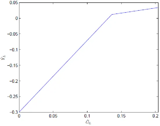
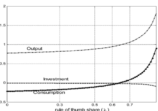
aggregate demand by increasing government spending. Figure 1 illustrates the relation between the level of government purchases and output.

The multiplier when government purchases are below their critical level is necessarily greater than 1. The main reason for this is that with the nominal interest at zero, an increase in increases expected inflation (given some positive probability of elevated credit spreads continuing for another period) and lowers the real rate of interest. Therefore monetary policy is even more accommodative than in the analysis of the previous chapter.

Figure 1: Output as a function of the level of government purchases during the period when the credit spreads remain elevated (Woodford 2010).

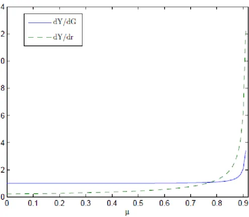
The degree to which the multiplier exceeds 1 can in this case be quite considerable. In fact, given a high enough value of the parameter , which is the probability that the credit spreads remain elevated during the following period and for any given

(34)

29

remains at zero bound can be unboundedly large. In general, though, the multiplier is not too much greater than 1 except when is fairly large. Figure 2 plots the multiplier as a function of . Note that the case in which is large is precisely the case in which the multiplier is also large, that is when a moderate increase in the size of credit spreads can cause a severe output collapse. Thus, at the zero lower bound increased government purchases should be a powerful means to help the economy recover from a crisis, especially when there is little confidence that the disturbance in the credit markets is short-lived (when is large).

Christiano et al. (2009) assume that the shock that makes the zero bound binding is an increase in the discount factor, which can be seen as representing a temporary

Figure 2: The derivatives of output with respect to real policy rate and for alternative values of (Woodford 2010, based partly on the parameter values of Eggertsson 2009).

(35)

30

rise in the agent’s propensity to save. In the model investment in the economy is assumed to be zero, so that aggregate saving must also be zero in equilibrium. If there is a large enough increase in the discount factor, the zero bound becomes binding before the real interest rate falls by enough to make aggregate saving 0. The only force that can induce the fall in saving required to re-establish equilibrium is a large transitory fall in output.

The explanation for such a large fall in output is as follows. Since the nominal interest rate is zero and expected inflation is negative, the real interest rate is positive. Both the increase in the discount factor and the rise in the real interest rate increase the

agent’s desire to save. There is only one force remaining to generate zero saving in equilibrium, a large transitory fall in income, which will lead to reduced desired saving as agents attempt to smooth their intertemporal consumption. Since this effect caused by a reduced desired level of saving has to counterbalance for the two factors leading agents to save more, the fall in income has to be very large.

With their benchmark specifications, the numerical value of the government spending multiplier is 3,7, which is roughly three times larger than in the previous chapter, where the interest rate was governed by a Taylor rule. The size of the multiplier does not depend on the size of the shock to the discount factor. The intuition for why the multiplier can be so large is that since an increase in government spending leads to a rise in output, marginal cost and inflation, and since with zero nominal interest rates the rise in expected inflation makes the real interest rate fall, private spending increases. This rise in expenditure generates a further rise in output, marginal cost and expected inflation and a further decline in the real interest rate, which will all result in a large rise in inflation and output.

When it comes to the sensitivity of the multiplier values to changes in different parameters, the longer the expected duration of the shock to the discount factor the higher the multiplier. Also, the multiplier is especially large in economies where the drop in output associated with the zero bound is large. In other words, fiscal policy is particularly powerful in economies where the output costs of being in the zero state bound are very large.

(36)

31

4.4 Discussion

In this chapter I have analyzed the size of the multiplier under three different assumptions about monetary policy. As a benchmark, I first considered a policy where the path of the real interest rate is held constant regardless of the level of government spending. In this case the multiplier equals 1 and there is no crowding out of private spending. The result, however, is not very useful since under realistic assumptions about monetary policy the real interest rate may change and it is hardly possible for the central bank to commit to a policy of this kind.

I then considered a situation, where the nominal interest rate is adjusted according to the Taylor rule and the real interest rate also varies along with the inflation rate. According to the model used by Christiano et al. (2009), private spending might not necessarily be crowded out in this case, but it can actually increase and the multiplier can be greater than one. The key assumption here is that consumption and leisure are complementary in preferences so that the marginal utility of consumption rises with employment and whenever this rise is large enough, multipliers larger than 1

are possible. The stickier the prices in the economy and the lower the central bank’s

response to increased inflation, the larger the multiplier.

After I moved on to consider perhaps the most interesting case when it comes to the analysis of the crisis, that is, when the nominal interest rate remains constant, which is relevant in the case of zero nominal interest rates. In all the three models considered here the multiplier is larger than 1 while the reasons behind the shocks are distinct. In the model by Eggertsson (2009) the crisis is caused by a deflationary shock, while Woodford (2010) considers a shock caused by financial disturbance and Christiano et al. (2009) a shock to the agents’ discount factor, which leads to

increased saving.

Based on the analysis seen here, fiscal stimulus can be useful in a crisis situation, especially if the government commits to sustaining a higher expenditure level as long as the crisis lasts, if there is disturbance in the financial markets which is experienced in the form of elevated credit spreads and the disturbance is likely to last for some