Optimizing multigrid smoothers using GLT theory

(1)

2020

Optimizing multigrid smoothers using

GLT theory

Denhanh Huynh

Department of Numerical Analysis, Lund University Master’s thesis supervised by Philipp Birken

(2)

2

Abstract

Multigrid algorithms are algorithms used to find numerical solutions to differen-tial equations using a hierarchy of grids of different coarseness. This exploits the fact that short-wavelength components of the solutions converges at a faster rate than the long-wavelength components when using some basic iterative methods, such as the Jacobi method or the Gauss-Seidel method. These iterative methods are also called smoothers since they have the effect of smoothing out the errors. In this thesis, two classes of smoothers based on time integration methods are studied using the one dimensional linear advection equation as model prob-lem. The first class is a class based on explicit Runge-Kutta methods, and the other class is derived from considering implicit Runge-Kutta methods. For both classes it is possible to derive a matrix M, dependent on the coefficient func-tion in the linear advecfunc-tion problem and the parameters of the smoother, which describes the evolution of the error. To optimize the smoothers parameters are chosen so that the eigenvalues ofMare optimized.

If the coefficient function is constant it is possible to derive a closed form expression for the eigenvalues of the resulting matrixM. However, in the vari-able coefficient case it is not possible, and for large matrices it is impractical to compute the eigenvalues using iterative methods. Therefore, the theory of

Generalized Locally Toeplitz (GLT) sequences is used to instead approximate the distribution of the eigenvalues. This results in an approximate optimiza-tion problem. The results show that this is an effective method for obtaining parameters for the smoothers in the variable coefficient case.

Popul¨

arvetenskaplig sammanfattning

M˚anga fysiska problem, s˚a som väderprognoser, luftflöden runt en flygplansvinge och vattenv˚agor, kan modelleras av differentialekvationer. Dessa kan inte alltid lösas analytiskt, men idag är v˚ara datorer kraftfulla nog att lösa m˚anga av dessa modeller numeriskt, dvs. genom att diskretisera problemet och approx-imera lösningen p˚a ett rutnät. Lösningarna för modellerna kan beskrivas som summor av v˚agor med l˚anga och korta v˚aglängder. När man använder simpla it-erativa lösare, ocks˚a kallade försmoothers, s˚a konvergerar de korta v˚aglängderna fortare än de l˚anga. Problemet med dessa lösare är just den l˚angsamma konver-gensen av de l˚anga v˚aglängderna. Dessa konvergerar snabbare om man använder grövre nät. Imultigrid-algoritmer använder man sig därför av flera rutnät av olika täthet för att f˚a snabb konvergens av b˚ade korta och l˚anga v˚aglängder av lösningen. Syftet med det här arbetet är att studera hur parametrar kan väljas för tv˚a andra typer av smoothers med hjälp av n˚agot kallat GLT-teori (Generalized Locally Toeplitz theory).

(3)

3

Acknowledgements

I would like to offer my sincere thanks to my supervisor Professor Philipp Birken at the Centre for Mathematical Sciences at Lund University. He consistently allowed this paper to be my own work, but steered me in the right the direction whenever he thought I needed it. He also helped improving my writing by offering valuable feedback.

I would also like to thank Dr. Fabio Durastante for helping me understand the article he coauthored, on which a lot of this thesis was based on.

Finally, I would like to thank my dear friend MSc Johan Book for his help, especially with the formulation in the popular science summary in Swedish.

(4)

(5)

Introduction

To find the numerical solution of unsteady flow problems one can use a multi-grid strategy. When using basic iterative methods to solve these problems, such as the Jacobi method or the Gauss-Seidel method, the short-wavelength components of the solutions converge faster than the long-wavelength compo-nents. Since this has the effect of smoothing out the error, these methods are called smoothers. The bottleneck of these methods is the slow convergence of the long-wavelength components. To circumvent this problem, multigrid algo-rithms uses several grids of different coarseness to speed up the convergence of the long-wavelength components.

These methods were shown by Caughey and Jameson [1] to be able to solve steady Euler flows in three to five multigrid cycles, which can be executed in a matter of seconds on a PC. However, with the multigrid strategy tuned for steady flow problems, the convergence rate for unsteady flow problems is deteriorated.

In [2], Birken showed that the convergence rate could be improved by opti-mizing the smoother of the multigrid method to unsteady flow problems. For this Birken used a class of smoothers based on explicit Runge-Kutta (RK) schemes, referred to as RK smoothers, which have low storage costs and scale well in parallel. It is possible to derive a matrix M created from the stability polynomial of the Runge-Kutta scheme which describes how the error evolves with each smoothing step. The RK smoothers are optimized by choosing pa-rameters for the RK scheme such that the eigenvalues of M(corresponding to the short-wavelength components) are minimized. Thus, the optimization of these smoothers requires knowledge about the eigenvalues ofM.

The constant coefficient linear advection equation, considered in [2], results in a matrixMfor which an explicit expression for the eigenvalues can be deter-mined analytically. However, this is not possible in the variable coefficient case, and if very fine grids are considered in the discretization of the problem, it is impractical to solve for the eigenvalues iteratively, since the matrices are large. Therefore, Bertaccini et al. proposed using the theory of Generalized Locally Toeplitz (GLT) matrix sequences [3] to instead approximate the distribution of

(8)

8 CHAPTER 1. INTRODUCTION

the eigenvalues and thus generalizing the strategy to variable coefficient convec-tion–diffusion equations [4].

GLT matrix sequences are built up by combining Locally Toeplitz sequences which in turn are generalizations of Toeplitz matrix sequences. A GLT sequence is described by a function, called the symbol of the GLT sequence. This symbol describes the asymptotic singular value distribution of the matrix sequence. With some additional assumptions on the matrices in the sequence, the symbol also describes the asymptotic eigenvalue distribution of the sequence.

The optimization of two different classes of smoothers is studied, using the GLT theory, with the one dimensional variable coefficient linear advection equa-tion as model problem. The first one is the class of explicit Runge-Kutta smoothers as mentioned above, and the other one is a class of W-smoothers (the convective part of the additive W-methods in [5]) which is a smoother de-veloped from considering implicit Runge-Kutta schemes. There is no unique set of optimal parameters for these smoothers that work for all problems [2], so improving the method of solving for the parameters plays a role in the efficiency of these smoothers.

In chapter 2 the model problem and the discretization of the problem is described in detail. The discretization of the model problem results in a linear system of the formAu=b. Chapter 3 explains how to solve this system using multigrid methods. The RK smoothers are described in chapter 4 as well as how to optimize them in the constant coefficient case. In chapter 5 the GLT theory is explained. Here, the eigenvalue distribution of matrices of different sizes from the same GLT sequence are compared to the symbol of the matrix sequence to see how well the symbol approximates the distribution of the eigenvalues of the matrices. Different coefficient functions result in different GLT sequences and symbols. Therefore, this is done for some different coefficient functions. The GLT theory is used to set up an approximate optimization problem for the parameters of the RK smoothers in the variable coefficient case in chapter 6. Here, a method for creating a lookup table for the parameters of the smoothers is also proposed. Chapter 7 introduces the W-smoothers, and describes how to optimize these smoothers, both in the constant coefficient case and the variable coefficient case. Numerical results are given with some discussion in chapter 8. Finally, some conclusions are given in chapter 9.

(9)

Chapter 2

Model problem and

discretization

The model problem used in this thesis is the one dimensional linear advection equation with periodic boundary conditions, i.e.

ut(x, t) + (a(x)u(x, t))x= 0, a(x)>0, a(x)∈R∀x∈[xmin, xmax], (2.1)

u(x=xmin, t) =u(x=xmax, t), (2.2)

which describes the bulk motion of a wave, and can be solved given an initial value

u(x, t= 0) =u0. (2.3)

In the above equation, the subscriptst andxrefers to partial derivatives with respect to the time variable tand spatial variablex.

2.1 Constant coefficient advection equation

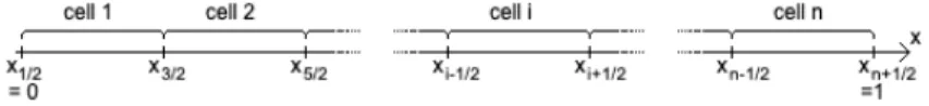
Here, the boundaries of xare set toxmin = 0 andxmax = 1 for simplicity, as

this can be done without loss of generality. To solve (2.1) numerically, the grid is discretized using n+ 1 equidistant grid points creating ngrid cells of width ∆x= 1/n(Figure 2.1). Here the grid pointsxi+1/2are defined asxi+1/2=i∆x,

where half integers are used so that grid celliranges fromxi−1/2toxi+1/2. The

boundary grid points corresponding to 0 and 1 are thusx1/2= 0 andxn+1/2= 1.

Figure 2.1: Discretization of the grid. 9

(10)

10 CHAPTER 2. MODEL PROBLEM AND DISCRETIZATION

First, the case where a(x) ≡ a is constant is considered. To get a finite volume scheme, the advection equation (2.1) is integrated over each grid cell:

0 = Z xi+1/2 xi−1/2 ut(x, t)dx+ Z xi+1/2 xi−1/2 (au(x, t))xdx = Z xi+1/2 x_i−1/2 ut(x, t)dx+a(u(xi+1/2, t)−u(xi−1/2, t))⇔ 0 = (ui(t))t+ a ∆x(u(xi+1/2, t)−u(xi−1/2, t)), i= 1,2, ..., n, (2.4)

whereuiis the cell average of celli, i.e. ui(t) := _∆x1

Rxi+1/2

xi−1/2 u(x, t)dx,i= 1, ..., n.

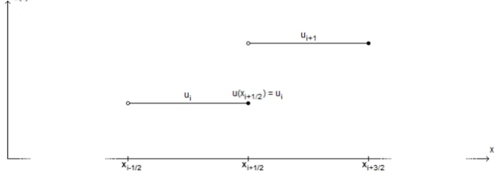
Let the solution vector be given byu= (u1, u2, ..., un)T = (u1(t), u2(t), ..., un(t))T,

which represents a step function (Figure 2.2).

Figure 2.2: Part of the solution vector u = (u1, u2, ..., un)T. The value of

u(xi+1/2) is chosen to be represented by the value of the step function on the

left side, i.e. ui.

To represent u(xi+1/2) and u(xi−1/2) in terms of the values of this step

function, one must choose to either use the value of the step function on the left or right side of the grid point. Using an upwind scheme, the function evaluations are weighted towards the side where the information is coming from. Since

a > 0, the wave is travelling in the positive x-direction. Therefore, the left value is chosen. This leads to the system of ODEs

(ui)t+

a

∆x(ui−ui−1) = 0, i= 1,2, ..., n, (2.5)

which is an approximation of (2.4). Here u0 := un because of the periodic

boundary conditions. This system of ODEs can be written in matrix form ut+

a

∆x

˜

(11)

2.2. VARIABLE COEFFICIENT ADVECTION EQUATION 11 where ˜Bn is ann×nmatrix given by

˜ Bn=        1 −1 −1 1 −1 1 . ._. . ._. −1 1        , (2.7)

and u= (u1, u2, ..., un)T as defined above. Let superscripts denote the current

time step. To get the fully discretized form of the linear advection equation, (2.6) is discretized in time using an implicit Euler step of size ∆t. This leads to the linear system

uk+1=uk+ ∆tuk+1_t =uk−a∆t ∆x ˜ Bnuk+1⇔ In+ a∆t ∆x ˜ Bn uk+1=uk ⇔ ˜ Anuk+1=uk, (2.8) where ˜ An:=In+ a∆t ∆x ˜ Bn. (2.9)

Here In denotes then×nunit matrix.

2.2 Variable coefficient advection equation

If a is not assumed to be constant (still witha(x)>0∀x), the finite volume upwind scheme for (2.1) becomes

(u1)t+ 1 ∆x(a1+1/2u1−an+1/2un) = 0 (ui)t+ 1 ∆x(ai+1/2ui−ai−1/2ui−1) = 0, i= 2, ..., n, (2.10)

where ai+1/2:=a(xi+1/2), and the corresponding matrix form is given by

ut+ 1 ∆xBnu=0, (2.11) where Bn =        a3/2 0 . . . −an+1/2 −a3/2 a5/2 −a5/2 a7/2 . ._. . ._. −an−1/2 an+1/2        . (2.12)

(12)

12 CHAPTER 2. MODEL PROBLEM AND DISCRETIZATION

As in the constant coefficient case, (2.11) is discretized in time with implicit Euler and time step ∆t, which leads to the fully discretized form

uk+1=uk+ ∆tuk+1_t =uk− ∆t ∆xBnu k+1_⇔ Anuk+1=uk, (2.13) where An =In+ ∆t ∆xBn. (2.14)

Note that for a constant a, the matrix Bn is simply aB˜n, which results in

(13)

Chapter 3

Multigrid methods

To solve the linear system (2.13) for the next stepuk+1_{, one can use} _multigrid methods [6, 7]. The aim of this section is to explain what multigrid methods are and why they are used.

3.1 Iterative methods

At each time step, a linear system of the form

Au=b (3.1)

has to be solved foruwhereu=uk+1_{, and}_b₌_uk _{is known from the previous}

time step. The subscript of A = An describing the size of the matrix has

been removed to simplify the derivations. Here the focus will be on solving this system using iterative methods. Let u denote the exact solution of (3.1) and letxdenote the current approximation ofu. The error is then defined as

e=u−x. (3.2)

For the constant coefficient case (2.9), the eigenvectors ofA= ˜A are given by the Fourier modes v˜j = (˜vj,1, ...,v˜j,n)T with ˜vj,l = eij

2πl

n . The error can be

described in terms of these Fourier modes e=

n/2

X

j=−n/2+1

cjv˜j, (3.3)

and it can be shown that, whenArepresents the discretization of a differential equation, iterating towarduusing a simple method such as the Jacobi method or the Gauss-Seidel method, the error components with high frequencies (cj˜vj

where |j| is high) are damped considerably faster than components with low frequencies (cjv˜j where|j|is low) [6, 7].

(14)

14 CHAPTER 3. MULTIGRID METHODS

Since |j| ∈ [0, n/2], let high frequency components of the error be defined as the components cj˜vj with |j| ≥ n/4 and let low frequency components of

the error be defined as the components with|j|< n/4, so that (approximately) half the components are defined as high frequency components and (approxi-mately) half are defined as low frequency components. One way to see that it is reasonable that the high frequency components are damped faster, in both the constant coefficient and the variable coefficient case, is through equations (2.5) and (2.10). High frequency error components corresponds to short distance er-rors (short wavelengths) and the low frequency error components correspond to long distance errors (long wavelengths). At each step of the iteration, the time derivative (ui)tof a cell is only affected by the values of the neighbouring cells.

Thus, it takes fewer iterations for the information to travel between cells with just a few cells between them and correct the local errors, than between cells with a large number of cells between them and correct the global error.

Since the high frequency components of the errors are eliminated faster than low frequency components, this has the effect of smoothing out the error. These iterative solvers are therefore also referred to assmoothers.

3.2 Coarse grid correction

The main idea behind multigrid algorithms is to speed up the convergence of the low frequency error components by the use of coarser grids, i.e. grids with less nodes, where the information travels farther with each step of the iteration. Some of the low frequency components of the error on the fine grid become high frequency components on the coarse grid.

Multiplying (3.2) with Afrom the left results in theresidual equation

Ae=Au−Ax=b−Ax⇔

Ae=r, (3.4)

showing that the error satisfies the same equation as ubut with the residual r := b−Ax on the right hand side instead of b. If the error was known exactly, then the solution of Au =b could be determined exactly since u = x+e. One method for improving the approximation x is thus to get a good approximation ¯eof the errorethrough the residual equation, and then updating the approximationxby

x←x+ ¯e. (3.5)

To speed up the convergence of the low frequency error components, instead of iterating on the fine grid, the residual is transferred to the coarse grid (explained in the next subsection) where the approximation of the error is computed. The error is then transferred back to the fine grid andxis updated using (3.5).

3.2.1 Restriction and prolongation

Leth= ∆xdenote the cell width for the original grid and create a coarser grid by removing every other grid point from the fine grid so that the coarse grid

(15)

3.3. TWO-GRID ALGORITHM 15 has half as many grid cells and the cell width 2h. To distinguish between the two grids, let the superscript of a matrix or vector denote the cell width of the grid on which it is evaluated. The vectors are transferred between the grids using the n₂ ×nrestriction matrixR (from fine to coarse grid) and then×n 2

prolongation matrixP(from coarse to fine grid) defined by

R=1 2      1 1 1 1 . ._. . ._. 1 1      , (3.6) and P= 2RT =               1 1 1 1 . ._. . ._. 1 1               . (3.7)

The vectorxh is thus transferred from the fine grid to the coarse grid by x2h=Rxh,

which corresponds to joining two adjacent cells by taking their average, and the vectorx2h _{is transferred from the coarse grid to the fine grid by}

xh=Px2h,

which corresponds to splitting one cell into two by duplicating the value of the cell. These transfer operations conserves the integral of the corresponding step functions over the spatial domain.

3.3 Two-grid algorithm

A multigrid method with two grids or levels, one fine grid (the top level) and one coarse grid (bottom level), could be implemented as follows:

1. Choose an initial guessxh_.

2. Presmoothing: Perform a number of smoothing steps onxh_.

3. Calculate the residualrh=bh−Ahxh. 4. Coarse grid correction:

(16)

(a) Restrict the residual to the coarse grid: rh_→_r2h₌_Rrh_.

(b) Restrict the matrixAh to the coarse grid: Ah→A2h.

(c) Solve for the errore2h _{on the coarse grid through the residual}

equa-tionA2he2h₌_r2h_.

(d) Prolong the error back to the fine grid: e2h→eh=Pe2h. (e) Updatexh throughxh←xh+eh

5. Postsmoothing: Perform a number of smoothing steps onxh.

Here, the matrix A2h is defined as the advection equation discretized on the coarse grid with ∆x= 2h.

3.4 V-cycle

To approximate the errore2h _{in step 4c one can use the same iterative method}

used for the smoothing in the presmoothing and postsmoothing steps. A good initial guess for the error is ¯e2h,(0)₌₀2h_{, since performing one smoothing step}

onxinAx=bwith initial guessxlis equivalent to performing one smoothing

step on the error el in Ael = rl with the specific initial guess ¯e (0)

l = 0 and

updatingxlusing (3.5) [6].

To show this for a linear method where A =N−NM and the next step xl+1 _{is given by}

xl+1=Mxl+N−1b (3.8)

(which is the case for methods such as the Jacobi method and the Gauss-Seidel method), let ¯e(1)_l denote the approximation of the erroreafter one smoothing step on ¯e(0)_l = 0, i.e. ¯e(1)_l = M¯e_l(0) +N−1rl ₌ _N−1_rl_{. Then the next step}

xl+1 _{when instead performing the smoothing step on the error and updating}

according to (3.5) is xl+1=xl+ ¯e(1)_l =xl+N−1rl =xl+N−1(b−Axl) =xl−N−1Axl+N−1b = (I−N−1A)xl+N−1b =Mxl+N−1b , (3.9)

which is the same as (3.8), proving that the two methods of updating xl are equivalent.

Using recursion, it is possible to speed up the convergence of the low fre-quencies of the error on the coarse grid by moving to even coarser grids with mesh widths 4h,8h, ...and so on until the grid is coarse enough, i.e. Ais small enough that Ae=r can be solved quickly with a direct method. This results in the following multigrid algorithm called aV-cycle.

(17)

3.5. STORAGE AND COMPUTATIONAL COST 17 Algorithm 1:v cycle(x,A,b,ν1,ν2,level)

Result: Improved approximation ofx. if level >0 then

Presmoothing: x= smoother(x,A,b), ν1 times

Calculate residual: r=b−Ax Restrict residual: rrest = restrict(r)

Restrict matrix: Arest= restrict matrix(A)

Initiateeon the coarse grid: e=0 Compute approximation oferecursively:

e= v cycle(e,Arest,rrest,ν1,ν2,level−1)

Prolong and update: x=x+ prolong(e)

Postsmoothing: x= smoother(x,A,b), ν2 times

else

Solve directly forxin Ax=b

Again, the matricesA4h,A8h, ...on the coarser grids are created by discretiz-ing the problem on those grids. For effective use of algorithm 1 it is assumed that the coarsest grid has few enough grid points, i.e. thatA is small enough, thatAx=bcan be solved quickly with a direct method. If this is not the case, the bottom level of the V-cycle could instead consist of a number of smoothing steps.

3.5 Storage and computational cost

The amount of storage needed on the finest grid scales linearly with the grid size. Assume that the finest grid requiresN bytes of storage. Each subsequent grid requires half as much storage as the previous one, so if M grids are used, the total storage cost is given by

N 1 + 1 2+ 1 22 +...+ 1 2M−1 . (3.10)

This is a geometric sum with the upper bound

N

1−1 2

= 2N. (3.11)

The computational cost of the multigrid algorithm is commonly measured in

work units (WU) [6, 7]. 1 WU is defined as the cost of performing one smooth-ing step on the finest grid. The cost of intergrid transfer operations typically amounts to 10-20% of the cost of an entire cycle, and is usually neglected. If

ν1is the number of presmoothing steps andν2 is the number of postsmoothing

steps, then the computational cost of the finest grid is (ν1+ν2)WU. Each

subse-quent grid requires half as much computational work as the previous, resulting in a geometric sum with the upper bound

(ν1+ν2)WU

1−1 2

(18)

Thus, the cost of storage and computation for a V-cycle is less than twice the cost of storage and computation of the finest grid alone regardless of the number of grids used. These computations were made for the one dimensional case (since the model problem used here is the one dimensional linear advection equation). For more dimensions, the bounds are even better [6]. For example, the factor 2 in (3.11) and (3.12) become 4/3 for two dimensions and 8/7 for three dimensions.

(19)

Chapter 4

Explicit Runge-Kutta

smoothers

Now, except for the number of smoothing steps and the number of grids, the only thing left to define is what smoother to use, which is the main subject of this thesis. One class of smoothers studied in this thesis is a class of explicit Runge-Kutta methods (RK methods) following [2, 4].

4.1 Pseudo time stepping

Consider the initial value problem given by xt∗=f(x),

x0=x(t∗0).

(4.1) The time t∗ is written here with a star as superscript to show that this is a pseudo time introduced only for iterating towards the solution of Au=b. To use this to find the solution ofAu=b, letf(x) =b−Ax. Ifxt∗=f(x)→0 as t∗ → ∞, then Ax→b as t∗ → ∞. This is the case if the real part of the eigenvalues of A are positive [8], which they are for the matrices here. This can be proven using the Gershgorin Circle Theorem [9], which states that each eigenvalue of a complex square matrix M with elementsmij are located in at

least one of theGershgorin disks

Di:={z:|z−mii| ≤

X

j6=i

|mij|}. (4.2)

Lemma 1. The real part of the eigenvalues of the matrices A=An defined in

(2.14) are positive.

Proof. First of all, with B :=Bn from (2.12), LetλB,j be an eigenvalue of B

(20)

20 CHAPTER 4. EXPLICIT RUNGE-KUTTA SMOOTHERS

and letvj be the corresponding eigenvector. Then

A=I+ ∆t ∆xB⇔ Avj = I+ ∆t ∆xB vj = 1 + ∆t ∆xλB,j vj, (4.3)

and thus, the eigenvaluesλA,j of Aare given by

λA,j = 1 +

∆t

∆xλB,j j= 1,2, ..., n. (4.4)

Now, by looking at the Gershgorin disks ofBT (withB:=Bn from (2.12))

one can deduce that the real part of the eigenvalues ofBT, and therefore also ofB(since BandBT have the same characteristic polynomial

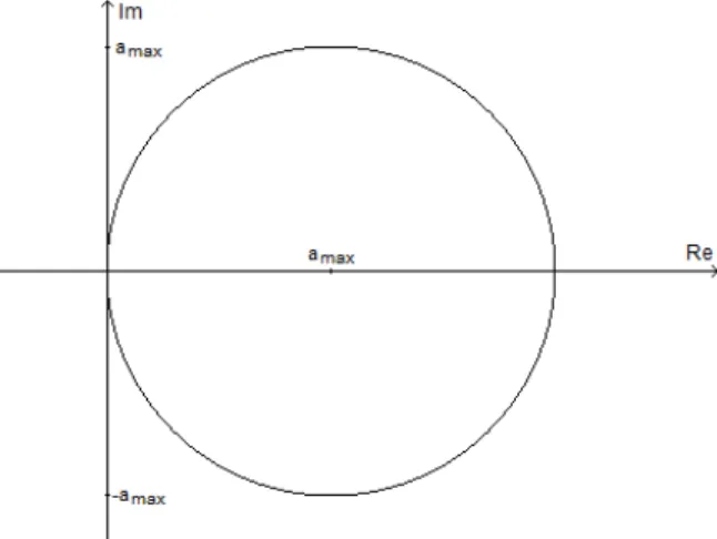
det(BT −λI) = det(BT−λIT) = det([B−λI]T) = det(B−λI), (4.5) they have the same set of eigenvalues), are non-negative: since the radii of the disks| −ai+1/2|=ai+1/2have the same value as the the centers of the disks on

the real axis, all disks are located in the right complex half-plane and intersect the imaginary axis at the origin. In particular, all eigenvalues ofB are located on or inside the circle with radiusamax:= maxxa(x)>0 and centered atamax

since all other Gershgorin disks are inside this circle (Figure 4.1). Therefore, since ∆t/∆x >0, it follows from (4.4) that the real part of the eigenvalues of Aare positive.

(21)

4.1. PSEUDO TIME STEPPING 21 The solution of (4.1) can be approximated with the explicit s-stage RK scheme given by x(0)_l =xl x(j)_l =xl+αj∆t∗f(x (j−1) l ), j= 1, ..., s−1 xl+1=xl+ ∆t∗f(x (s−1) l ) (4.6) where ∆t∗∈_Randαj∈[0,1]∀j.

One iteration of the RK smoother consists of taking one step in pseudo time

t∗ of size ∆t∗ using the RK scheme (4.6). Let αs = αs+1 = 1, and let the stability polynomial Ps(z) = s X r=0 s+1 Y m=s−r+1 αm ! zr, (4.7)

and the polynomial

Ss(z) = s−1 X r=0 s Y m=s−r αm ! zr, (4.8)

be defined. Then (4.6) can be described by

xl+1=Ps(−∆t∗A)xl+Ss(−∆t∗A)∆t∗b, (4.9)

which can be seen by working backwards: xl+1=xl+ ∆t∗(b−Ax (s−1) l ) =xl+ ∆t∗(b−A(xl+αs−1∆t∗(b−Ax (s−2) l ))) =... = " xl+ (−∆t∗A)xl+αs−1(−∆t∗A)2xl+...+ s−1 Y m=1 αm ! (−∆t∗A)sxl # + " ∆t∗b+αs−1(−∆t∗A)∆t∗b+...+ s−1 Y m=1 αm ! (−∆t∗A)s−1∆t∗b # = " I+ (−∆t∗A) +αs−1(−∆t∗A)2+...+ s−1 Y m=1 αm ! (−∆t∗A)s # xl + " I+αs−1(−∆t∗A) +...+ s−1 Y m=1 αm ! (−∆t∗A)s−1 # ∆t∗b =Ps(−∆t∗A)xl+Ss(−∆t∗A)∆t∗b. (4.10) From this it is possible to deduce that the RK smoothers satisfy (3.8) with M=Ps(−∆t∗A) andN−1=Ss(−∆t∗A)∆t∗. To show this,A=N−NMhas

to be proven. First, note that the relation

(22)

holds. This relation is shown as follows.

Ps(−∆t∗A) = s X r=0 s+1 Y m=s−r+1 αm ! (−∆t∗A)r =as+1(−∆t∗A)0+ " s X r=1 s+1 Y m=s−r+1 αm ! (−∆t∗A)r−1 # (−∆t∗A) =I−∆t∗ " s X r=1 s+1 Y m=s−r+1 αm ! (−∆t∗A)r−1 # A =I−∆t∗ "s−1 X r=0 s Y m=s−r αm ! (−∆t∗A)r # A =I−∆t∗Ss(−∆t∗A)A⇔ I−Ps(−∆t∗A) = ∆t∗Ss(−∆t∗A)A. (4.12) From this follows that

N−NM=N(I−M) = 1 ∆t∗Ss(−∆t ∗_A)−1_(I₋_P s(−∆t∗A)) = 1 ∆t∗Ss(−∆t ∗_A)−1_∆_t∗_S s(−∆t∗A)A =A, (4.13)

where (4.11) was used in the third equality.

4.2 Evolution of the error

Letube the solution toAu=band letxl be the current approximation ofu

as above. Also, let the errorel be defined as in (3.2), i.e. el =u−xl. Since

xl+1 =Mxl+N−1band A=N−NM⇔N−1 =A−1−MA−1, taking one

step with the RK smoother results in el+1=u−xl+1 =u−(Mxl+N−1b) =u−Mxl−N−1b =u−M(u−el)−(A−1−MA−1)b =u−Mu+Mel−(u−Mu) =Mel. (4.14)

(23)

4.3. OPTIMIZING M 23

4.3 Optimizing M

Letvjdenote the eigenvectors ofMand letλj denote the corresponding

eigen-values. If the error at stepkis described in terms of the eigenvectors ek=

n/2

X

j=−n/2+1

cj,kvj (4.15)

then the error aftermiterations is ek+m=Mmek = n/2 X j=−n/2+1 cj,kλmj vj. (4.16)

Here the eigenvectors ofAcreated from the variable coefficient case are assumed to approximately behave as the eigenvectors of ˜Ain the constant coefficient case, so the components cj,kvj will be referred to as high frequency components if

|j| ≥n/4 and low frequency components if|j|< n/4. To optimize the overall convergence of the smoother, one would need to minimize maxj|λj|with respect

to the parameters of the RK method, i.e. the coefficientsαi, i= 1, ..., s−1, and

the pseudo time step ∆t∗. However, since the low frequency components are handled by moving to a coarser grid in the multigrid method, the smoother is instead optimized for the convergence of the high frequency error components, i.e. to minimize the smoothing factor max|j|≥n/4|λj|, and the optimization

problem becomes min ∆t∗_,α 1,...,αs−1 max |j|≥n/4|λj| (4.17) with ∆t∗ _∈

Randαj ∈[0,1]∀j. Thus, to optimize the explicit RK smoother,

the eigenvalues ofM are needed.

4.4 Eigenvalues of M

Let Mn denote the matrix M of size n×n, i.e. Mn = Ps(−∆t∗An). Since

the eigenvectors of Mn are the same as the eigenvectors for An, and since

An =In+_∆x∆tBnis constructed using the matrixBn, the eigenvalues ofBn are

computed first.

4.4.1 Constant coefficient

In the constant coefficient case, the eigenvalues of the matrix ˜Bndefined in (2.7)

(24)

the first row and the last column from ˜Bn−˜λBIn, i.e.

D1,n=      −1 1−λ −1 1−λ . ._. . ._. −1      (4.18)

Then the determinant of this matrix is

det(D1,n) = (−1)n−1. (4.19)

Thus, by expanding det( ˜Bn−˜λBIn) along the first row:

det( ˜Bn−˜λBIn) = 0⇔ (1−λ˜B)n+ (−1)n+1(−1) det(D1,n) = 0⇔ (1−λ˜B)n−1 = 0⇔ ˜ λB,j= 1−exp −i2πj n , j∈Z:j∈(− n 2, n 2], (4.20)

where i is the imaginary unit. In this text, to distinguish the imaginary unit from the index, the imaginary unit i will always be non-italic.

Letvj be thejth eigenvector of ˜Bn. Then

˜ Anvj = In+ a∆t ∆x ˜ Bn vj = 1 + a∆t ∆x ˜ λB,j vj, (4.21)

and from this follows that the eigenvalues of ˜An are given by

˜ λA,j = 1 + a∆t ∆x ˜ λB,j = 1 +a∆t ∆x 1−exp −i2πj n , j∈_Z:j∈(−n 2, n 2]. (4.22) Finally, since Mnvj=Ps(−∆t∗A˜n)vj =Ps(−∆t∗λ˜A,j)vj, (4.23)

the eigenvalues ofMn are given by

˜ λP,j =Ps(−∆t∗˜λA,j) =Ps −∆t∗ 1 +a∆t ∆x 1−exp −i2πj n , j∈Z:j∈(− n 2, n 2]. (4.24)

(25)

4.4. EIGENVALUES OFM 25

4.4.2 Variable coefficient

In the variable coefficient case, it is not as easy to determine the eigenvalues. By following the same process above for the eigenvalues ofBn defined in (2.12),

one would end up at the following expression: det(Bn−λBIn) = n Y i=1 (ai+1/2−λB)− n Y i=1 ai+1/2= 0, (4.25)

for which there is no general solution in radicals forn≥5 (Abel’s impossibility theorem). While it is possible to approximate the eigenvalues using iterative methods, it becomes computationally expensive as the size of the matrix gets large.

In the next chapter it will be shown that it is possible to get an explicit expression that approximates how the eigenvalues of the matrices Bn and An

(26)

(27)

Chapter 5

Generalized Locally

Toeplitz Sequences

The theory ofgeneralized locally Toeplitz (GLT) sequences[3] can be used to get information about thedistribution of singular values, and given some additional assumptions, also thedistribution of eigenvalues, of large matrices.

In this text, amatrix sequenceis a sequence of the form{An}n, whereAn∈

Cn×n, andn∈N. All definitions in this chapter are taken from [3].

Definition 2. Let{An}n be a matrix sequence, and letf :D⊂Rk →Cbe a measurable function defined on a set D with 0< µk(D)<∞. Also letσi(An)

denote theith singular value andλi(An) denote theith eigenvalue of the matrix

An. Then

• {An}nhas asingular value distribution described byf, denoted by{An}n∼σ

f, if lim n→∞ 1 n n X i=1 F(σi(An)) = 1 µk(D) Z D F(|f(x)|)dx, ∀F ∈Cc(R). (5.1) (Cc(C) (resp., Cc(R)) refers to the space of complex-valued continuous functions defined on_C(resp.,_R) with bounded support.) f is then called thesingular value distribution symbol of{An}n.

• {An}n has a spectral (or eigenvalue) distribution described byf, denoted

by{An}n∼λf, if lim n→∞ 1 n n X i=1 F(λi(An)) = 1 µk(D) Z D F(f(x))dx, ∀F ∈Cc(C). (5.2)

f is then called thespectral (or eigenvalue) distribution symbol of{An}n.

(28)

28 CHAPTER 5. GENERALIZED LOCALLY TOEPLITZ SEQUENCES

What this means is that if{An}nhas a singular value distribution described

byf and ifnis large enough, then the singular valuesσi(An) are approximately

equal to the samples of |f| over a uniform grid inD, and equivalently for the eigenvaluesλi(An) andf, if{An}n has an eigenvalue distribution described by

f.

The aim of this chapter is to give an understanding of GLT sequences. An explanation ofToeplitz sequencesis given in section 5.1. This is then generalized intolocally Toeplitz (LT) sequencesin section 5.2, and finally into GLT sequences in section 5.3. Some properties, including asymptotic eigenvalue and singular value distributions of GLT sequences are given in subsection 5.3.1.

In this text, amatrix sequenceis a sequence of the form{An}n, whereAn ∈

Cn×n, andn∈N.

5.1 Toeplitz sequences

Recall the matrix

˜ Bn=        1 −1 −1 1 −1 1 . ._. . ._. −1 1       

that arose in the semi-discretized form of the constant coefficient case (2.6). This is a special type of matrix called aToeplitz matrix.

Definition 3. A matrixAwhere each diagonal is constant:

A= [aj−i]ni,j=         a0 a1 a2 . . . an−1 a−1 a0 a1 a−2 a−1 a0 . .. .. . . .. . .. a1 a₋(n−1) a−1 a0         (5.3)

is called aToeplitz matrix.

A Toeplitz matrix can be defined by a functionfusing Fourier analysis. The reason for doing this is that the functionf also contains information about the eigenvalues of the Toeplitz matrix, as will be seen in section 5.3.

(29)

5.2. LOCALLY TOEPLITZ SEQUENCES 29 Thenth Toeplitz matrix associated withf, denotedTn(f), is defined as

Tn(f) = [fj−i]ni,j=1=         f0 f1 f2 . . . fn−1 f−1 f0 f1 f−2 f−1 f0 . .. .. . . .. . .. f1 f−(n−1) f−1 f0         , (5.4)

where fk is thekth Fourier coefficient off:

fk = 1 2π Z π −π f(θ)e−ikθdθ. (5.5) The matrix sequence {Tn(f)}n is called theToeplitz sequence generated byf.

Given a Toeplitz matrix, the functionf can be easily found as a Fourier series with Fourier coefficients given by the elements of the matrix. For example, the matrix ˜Bnis thenth Toeplitz matrix associated withf(θ) = 1−e−iθ−ei(n−1)θ.

5.2 Locally Toeplitz sequences

In the variable coefficient case, the matrix describing the semi-discrete form (2.11) was Bn =        a3/2 0 . . . −an+1/2 −a3/2 a5/2 −a5/2 a7/2 . ._. . ._. −an−1/2 an+1/2        .

Ifa(x) is not constant, then this is not a Toeplitz matrix. However, asn→ ∞ it resembles the structure of a toeplitz matrix locally in the sense that small subblocks ofBn are close to being Toeplitz matrices. To defineLocally Toeplitz sequences rigorously, a number of other definitions first have to be made.

Definition 5. Let a: [0,1]→ C, and letn ∈ N. The nth diagonal sampling

matrix generated by a, denotedDn(a), is defined as

Dn(a) = diag i=1,...,n a(i n) =      a(1_n) a(_n2) . ._. a(1 n)      . (5.6)

(30)

Definition 6. Let m, n∈N, a: [0,1]→C, and f ∈L1([−π, π]). Thelocally

Toeplitz operators ofaand f are defined as the followingn×nmatrices:

LT_nm(a, f) =D(a)⊗Tbn

mc(f)⊕Onmodm, (5.7)

where the tensor (Kronecker) product ”⊗” is applied before the direct sum ”⊕”, i.e. LT_nm(a, f) =        a(1 m)Tbmnc(f) a(2 m)Tbmnc(f) . ._. a(1)Tbn mc(f) Onmodm        . (5.8) HereOn denotes then×nzero matrix, andb·c denotes the floor function.

Note that each block a(_mi )Tbn

mc(f) in (5.8) is a Toeplitz matrix, and that

every Toeplitz matrix Tn(f) is also a locally Toeplitz operator with Tn(f) =

LTm

n (1, f) for anym∈N.

The matrixBn is not a locally Toeplitz operator which can be easily seen by

noting that the matrixBnis not a blockdiagonal matrix. However, it resembles

a locally Toeplitz operator as n→ ∞. This resemblance can be defined using the concept ofapproximating classes of sequences.

Definition 7. Let {An}n be a matrix sequence and let{{Bn,m}n}m be a

se-quence of matrix sese-quences. Then {{Bn,m}n}m is an approximating class of sequences (or a.c.s.) for{An}n if the following property holds: ∀m∃nm:n≥

nm⇒

An =Bn,m+Rn,m+Nn,m, rank(Rn,m)≤c(m)n, ||Nn,m|| ≤ω(m), (5.9)

where the quantitiesnm, c(m), andω(m) only depend onm, and

lim

m→∞c(m) = limm→∞ω(m) = 0.

This is denoted by{{Bn,m}n}m a.c.s.

−−−→ {An}n.

Thus, if{{Bn,m}n}mis an approximating class of sequences for{An}n and

n and m are large, then the matrix An is equal to the matrix Bn,m plus two

matrices that are close to the zero matrix in two different ways:

• The matrix Rn,mhas a low rank relative to the size of the matrix.

• The matrix Nn,m has a small norm. (Any norm, since all norms are

(31)

5.3. GENERALIZED LOCALLY TOEPLITZ SEQUENCES 31 Given these definitions,Locally Toeplitz sequences can now be defined.

Definition 8. Let{An}n be a matrix sequence, leta: [0,1]→Cbe Riemann integrable, and let f ∈ L1_([−_{π, π}_{]). Then} _{_A

n}n is a locally Toeplitz (LT) sequence with symbola⊗f, denoted by{An}n∼LT a⊗f, if

{LT_nm(a, f)}n a.c.s.

−−−→ {An}n.

Here a⊗f is the tensor-product ofaandf, i.e. (a⊗f)(x, θ) :=a(x)f(θ).

The matrix sequence{Bn}n created by Bn is an LT sequence with symbol

κB(x, θ) =a(x)(1−exp(−iθ)), (5.10)

i.e. {Bn}n ∼LT κB(x, θ) as shown in [4]. (The matrices in the matrix

se-quence this was shown for had a different first row. However, the difference between the matrices could be added into the matrix Rn,m in the definition of

an approximating class of sequences.)

5.3 Generalized Locally Toeplitz sequences

The concept of LT sequences can be further generalized by combining different LT sequences.

Definition 9. Let{An}n be a matrix sequence, and letκ: [0,1]×[−π, π]→C be a measurable function. Then {An}n is a generalized locally Toeplitz (GLT) sequence withsymbol κ, denoted by {An}n ∼GLT κ, if the following property

holds: ∀m ∈ N there exists a finite number of LT sequences {A(i,m)n }n ∼LT

ai,m⊗fi,m, i= 1, ..., Nmsuch that

• PNm

i=1ai,m⊗fi,m→κin measure, and

• PNm i=1{A (i,m) n }n a.c.s. −−−→ {An}n.

Any linear combination of LT sequences is a GLT sequence, since then the above condition holds with Nm constant for allm (note that an LT sequence

multiplied by a scalar is an LT sequence). In particular, every LT sequence {An}n∼LT κ=a⊗f is also a GLT sequence.

(32)

5.3.1 Properties of GLT sequences

If a sequence of matrices is a GLT sequence and the symbol of the GLT sequence is known, then thesingular value distribution, and with additional assumptions also the eigenvalue distribution, of the matrix sequence is known. Here follow some useful properties of GLT sequences given in [3].

Proposition 10. The following properties hold for GLT sequences:

GLT1 If {An}n ∼GLT κ then {An}n ∼σ κ. If in addition the matrices An

are Hermitian, then{An}n ∼λκ.

GLT2 If {An}n ∼GLT κ and each matrix An can be separated into An =

Xn+Yn where

• eachXn is Hermitian,

• ||Xn||,||Yn|| ≤C for some constant C independent ofn, and

• ||Yn||1/n→0 asn→ ∞,

then{An}n ∼λκ.

GLT3The following hold:

• {Tn(f)} ∼GLT κ(x, θ) =f(θ) forf ∈L1([−π, π]),

• {Dn(a)}n ∼GLT κ(x, θ) =a(x) for a: [0,1]→Chereais continuous a.e., and • {Zn}n∼GLT 0 if and only if{Zn}n∼σ0. GLT4If{An}n∼GLT κand{Bn}n ∼GLT ξ, then • {A∗_n}n∼GLT ¯κ • {αAn+βBn}n ∼GLT ακ+βξ ∀α, β∈C • {AnBn}n∼GLT κξ

GLT4 is equivalent to stating that the space of GLT sequences forms a *-algebra of matrix sequences. GLT3 and GLT4 can be used to determine the symbol of a matrix sequence, and GLT1 and GLT2 are used for getting information about the singular values and eigenvalues of matrix sequences for which the symbol is known. Points 2 and 3 fromGLT4can be used to give the following useful corollary.

Corollary 11. Let {An}n ∼GLT κ and let P be a polynomial. Then the

(33)

5.4. SYMBOLS OF {AN}N AND{BN}N 33 Proof. Applying the third point from GLT4 multiple times leads to the formula

{Ak_n}n∼GLT κk. (5.11)

Let the degree of the polynomialP be denoted by s and letak, k = 0, ..., s

denote the coefficients of the polynomial. Then applying the second point from GLT4 (linearity) in addition to (5.11) leads to

{P(An)}n={ s X k=0 akAkn}n∼GLT s X k=0 akκk=P(κ). (5.12)

Thus, if the symbol of the matrix sequence{An}n is known, the symbol of

{P(An)}n is also known.

To optimize a smoother, one would preferably like to know the eigenvalue distribution of the matrix sequence in addition to knowing the singular value distribution (which will be seen to be the case for the matrix sequences in this thesis). However, since the eigenvalues are bounded by the largest singular value

|λj| ≤max

i σi ∀j∈[1, n], (5.13)

it is still possible to get useful information about the eigenvalues even if only the singular value distribution is known.

5.4 Symbols of

{A

n

}

n

and

{B

n

}

n

As stated above, the matrix sequence{Bn}n withBn defined as in (2.12) is an

LT sequence with symbol

κB(x, θ) =a(x)(1−exp(−iθ)). (5.14)

Since all LT sequences are also GLT sequences, this is also a GLT sequence. From this follows that {Bn}n ∼σ κB(x, θ) by GLT1 in proposition 10. Since

these matrices are not Hermitian, the sequence does not satisfy the second part of GLT1. However, it does satisfy GLT2 by seperating each Bn into Bn =

Xn+Yn where Xn :=        a3/2 a5/2 a7/2 . ._. an+1/2        (5.15)

(34)

is Hermitian sincea(x)∈R, and

Yn:=        0 −an+1/2 −a3/2 0 −a5/2 0 . ._. . ._. −an−1/2 0        . (5.16)

Since all norms are equivalent, it is enough that||Xn||and ||Yn||are bounded

with respect to the 1-norm, which they are with the bound C = maxxa(x).

Since||Yn||1is bounded byC it also follows that||Yn||1/n n→∞

−−−−→0. Thus {Bn}n∼λκB(x, θ) (5.17)

by GLT2.

By GLT3 the symbol of the identity matrix In is simply 1. If ∆t/∆x is

assumed to be constant, then by GLT4 the matrix sequence {An}n defined in

(2.14), i.e. {An}n = In+ ∆t ∆xBn n ,

is a GLT sequence with the symbol

κA(x, θ) = 1 + ∆t ∆xκB(x, θ) = 1 + ∆t ∆xa(x)(1−exp(−iθ)). (5.18)

Even if {An}n did not satisfy the additional assumptions given in GLT1 or

GLT2 for the symbol to describe the eigenvalue distribution, it is still true that {An}n ∼λ κA(x, θ). This can be seen by looking at the eigenvalues ofAn for

a fixed n and then letting n tend to infinity. As was deduced in (4.4), the eigenvalues ofAn are given by

λA,j = 1 +

∆t

∆xλB,j j= 1,2, ..., n.

Since this is true for alln, it follows that the asymptotic eigenvalue distribution ofAn is given by

1 + ∆t

∆xκB(x, θ) =κA(x, θ). (5.19)

Note that this would be true whether{An}n was a GLT sequence or not.

For the different levels of the multigrid algorithm, the value of ∆t/∆x is doubled and halved when moving between levels (since ∆t is fixed and ∆x

is doubled when moving to a coarser grid). To get the approximation of the eigenvalue distribution of a matrixAn for a given level, one would have to fix

∆xand use the symbol for the corresponding matrix sequence. Here, with some abuse of notation, the eigenvalue distribution of the sequence{An}n with ∆x=

1/ndependent onnwill be said to have an eigenvalue distribution described by

(35)

5.5. NUMERICAL EXAMPLES 35

5.5 Numerical examples

To see how closely the eigenvalues are distributed according to the symbol for various n, or at least how well the eigenvalues covers the image of the symbol, some numerical tests were done. The values

xmin= 0,

xmax= 2, and

∆t= 3/25,

were used for the discretization in all examples below. For each test, defined by which functiona(x) that was used, matricesAnof sizen= 128,1024,4096,8192

were created. The eigenvalues were then computed in python using the function scipy.linalg.eig from the SciPy library.

5.5.1 Sine function

The first test was done with the function

a(x) = 1 + 0.7 sin

₄_πx

xmax−xmin

(5.20)

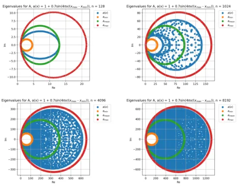
(Figure 5.1). Figure 5.2 shows plots of the eigenvalues of An for the various

n. The orange, green and red points show the eigenvalues for the matrix in the constant coefficient case, where the constant a = amin, a = amean, and

a =amax respectively. Remember that these eigenvalues are given exactly by

the explicit expression in (4.22). The area between the orange and the red circles corresponds to the image of the symbolκA(x, θ). Note that since ∆x= 2/n is

changed with increasingn, the ranges for the eigenvalues are also changed with

n.

As expected from the GLT theory, the distribution of the eigenvalues gets closer to the image with increasing n. For values of n < 128, all eigenvalues were located inside the green circle created from the eigenvalues for An with

(36)

Figure 5.1: The functiona(x) = 1 + 0.7 sin_x 4πx

max−xmin

along with lines repre-senting the maximum, the minimum, and the mean ofa(x).

Figure 5.2: Eigenvalue plots for A128, A1024, A4096, and A8192, created by

a(x) = 1 + 0.7 sin_x 4πx

max−xmin

(37)

5.5.2 Monotone convex function

The second test was done with the function

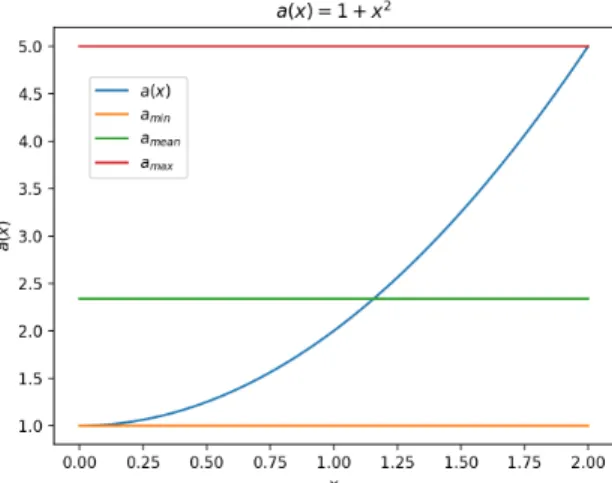
a(x) = 1 +x2 (5.21)

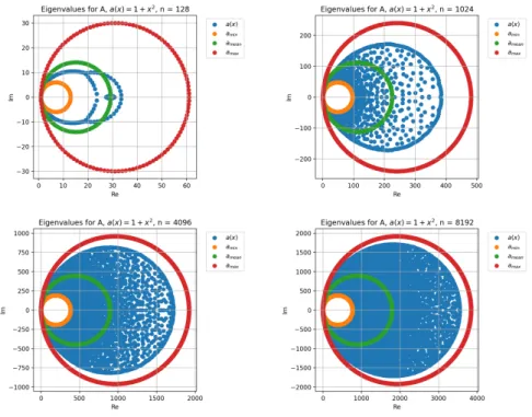
(Figure 5.3). The result is shown in Figure 5.4. As expected, the distribution get closer to the image ofκA(x, θ) asnis increased in this case as well.

For this coefficient function, the eigenvalues are outside of the green circle even for low values ofn(even fornas low asn= 4). Another result that differs from the sine function case is that the eigenvalue distribution converges more slowly towards the red circle. A possible reason for these results is that the mean ofa(x) amean= 1 2 Z 2 0 1 +x2dx=1 2 x+x 3 3 2 0 = 7 3 ≈2.33 (5.22) shown as the green line in Figure 5.3 is below the midpoint 3 of the range of the function a(x)∈[1,5]. This means that the point evaluationsai+1/2 for the

discretized version ofa(x) are weighted towards the lower half of the range. For this reason, a third test was done with a concave function.

Figure 5.3: The function a(x) = 1 +x2 _{along with lines representing the}

(38)

a(x) = 1 +x2_.

5.5.3 Concave function

The third test was done with the function

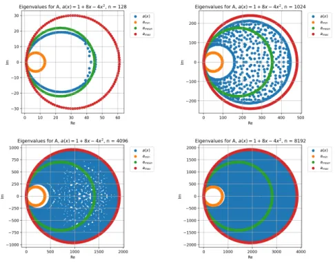
a(x) = 1 + 8x−4x2 (5.23) (Figure 5.5). This function is a concave function that was chosen to have the same range as the monotone convex function a(x) ∈[1,5]. Here, the mean of

a(x) amean= 1 2 Z 2 0 1 + 8x−4x2dx= 1 2 x+ 4x2−4x 3 3 2 0 = 11 3 ≈3.67 (5.24) is above the midpoint 3 of the range. The eigenvalue distributions for this function are shown in Figure 5.6. As suspected, the distribution in this case converges faster towards the red circle and slower towards the orange circle compared to both the sine function, and the monotone convex function case. Overall the convergence seems to be the fastest for the concave function case. This is not necessarily true in general for GLT sequences, but is the case here for this discretization of the linear advection equation. The key point here is that the convergence of the eigenvalues towards the image of the domain through the symbol depends ona(x) even if they result in the same image of the symbol.

(39)

Figure 5.5: The function a(x) = 1 + 2x−x2 along with lines representing the maximum, the minimum, and the mean of a(x).

(40)

Remark. A question that arises is whether it can be assumed that all eigen-values are located within the image of the symbol as they appear to do for the examples given here. That all eigenvalues are located on or inside the red circles in Figures 5.2, 5.4, and 5.6, can be proven by again turning to the Gershgorin circle theorem. Given a coefficient functiona(x), the eigenvalues of the resulting matrixBn are located on or inside the circle centered atamax, as was stated in

section 4.1. Since the eigenvalues ofAn are given by (4.4), i.e.

λA,j = 1 +

∆t

∆xλB,j j= 1,2, ..., n,

the eigenvalues ofAn must all be located on or inside the circle centered at

1 + ∆t ∆xamax

(41)

Chapter 6

Optimizing explicit

Runge-Kutta smoothers

Using the theory of GLT sequences it is now possible to approximate the distri-bution of the eigenvalues of Mn=Ps(−∆t∗An) withAn defined as in (2.14).

6.1 Symbol of

{M

n

}

n

By Corollary 11, the symbol of the matrix sequence{Mn}n is

κM(x, θ) =Ps(−∆t∗κA(x, θ)) =Ps −∆t∗ 1 + ∆t ∆xa(x)(1−exp(−iθ)) . (6.1)

If a(x)≡a is constant and ifθ only takes the discrete valuesθ = 2πj/n, j ∈ Z:j ∈(−n2,

n

2], then this becomes the same expression as (4.24), which is the

exact expression for the eigenvalues of Mn in the constant coefficient case.

Since xt∗ = b−Ax → 0 as t∗ → ∞, one would ideally want to take as large pseudo time steps ∆t∗as possible. Since these smoothers are created from explicit schemes, the pseudo time step ∆t∗is restricted by a CFL condition [10] dependent on the coefficient function and the discretization of the function.

Let r:= ∆t ∆x, (6.2) c:= ∆t ∗_∆_t ∆x , (6.3) and define z(c, x, θ;r) :=−c r−ca(x)(1−exp(−iθ)). (6.4)

The symbol can then be written as

κM(x, θ) =Ps(z(c, x, θ;r)). (6.5)

(42)

42CHAPTER 6. OPTIMIZING EXPLICIT RUNGE-KUTTA SMOOTHERS

Using the variables randc avoids some divisions and multiplications with po-tentially very small numbers in addition to simplifying the expression. Thus, instead of optimizing directly for ∆t∗ here, ∆t∗ is instead solved from the opti-mized value ofc in (6.3), which is a value closely related to the CFL condition. With the same idea as in subsection 5.4, to see that the eigenvalue distribution of {Mn}n is given by its symbol, letvA be an eigenvector of An with nfixed

and letλA be the corresponding eigenvalue. Then the following holds

MnvA=Ps(−∆t∗An)vA=Ps(−∆t∗λA)vA. (6.6)

Since this is true for each fixedn, it follows that (by letting ntend to infinity) {Mn}n∼λPs(−∆t∗κA(x, θ)) =Ps(z(c, x, θ;r)). (6.7)

Hence, convergence of the RK smoother requires that parameters are chosen so that

max

x,θ |Ps(z(c, x, θ;r))|< Hn, (6.8)

for a boundHn defined by

Hn:=

maxx,θ|Ps(z(c, x, θ;r))|

|λmax(Mn)|

n→∞

−−−−→1, (6.9) as this would imply that|λmax(Mn)|<1.

6.2 Approximate optimization problem

The parameters of the s-stage RK smoother to optimize are the coefficients

αi, i= 1, ..., sand c. The approximate optimization problem becomes

min c,α1,...,αs max (x,θ)∈[xmin,xmax]×[π/2,π] |Ps(z(c, x, θ;r))| , (6.10)

where ∆t∗ is solved fromc by ∆t∗ := c∆x_∆t . The domain forθ is cut down to [π/2, π] for the following reasons. Firstly, to optimize for the convergence of high frequency components, the domain [−π, π] is cut in half into [−π,−π/2]∪[π/2, π] (this corresponds to |j| ≥n/4 in the discrete case). Secondly, since |Ps(z)| =

|Ps(z)|, wherezis the complex conjugate ofz, and since the complex conjugate

of exp(−iθ) is exp(iθ), the domain [−π,−π/2]∪[π/2, π] is cut in half once again into [π/2, π].

6.2.1 Parameters from optimization problem on coarse

grids

Since the eigenvalue distribution results from the GLT theory are asymptotic, there is no guarantee that the parameters ∆t∗_{, α}

1, ..., αsobtained from the

(43)

6.2. APPROXIMATE OPTIMIZATION PROBLEM 43 if all of the eigenvalues are located within the image given by the symbol, as they were in the numerical examples above, then

max

x,θ |Ps(z(c, x, θ;r))| ≥ |λmax(Ps(−∆t

∗_A

n)| (6.11)

and the parameters should at least guarantee convergence (of the high frequency components) if the value of maxx,θ|Ps(z(c, x, θ;r))| is below one, i.e. Hn ≥1

in (6.8). That all eigenvalues are at least located on or inside the red circles in Figures 5.2, 5.4, and 5.6, was proven in the remark in section 5.5.

6.2.2 Invariance of parameters on fine grids

One thing to note is that if the grids are fine enough, i.e. if nis large enough, so that 1/r= ∆x/∆t∝1/nis small relative toa(x)(1−exp(−iθ)), then

z(c, x, θ;r) :=−c

r−ca(x)(1−exp(−iθ)≈ −ca(x)(1−exp(−iθ)). (6.12)

Sincez(c, x, θ;r) is then approximately independent ofr, and therefore the cell width ∆x, the optimal parameters c, α1, ..., αs are approximately constant on

different levels of the multigrid algorithm. Thus, if a fine enough grid is used for the discretization of the problem, it is potentially not necessary to solve the problem for every level of the algorithm. The only parameter that needs to be changed for the RK smoother between levels with a largenis then

∆t∗= c∆x

∆t (6.13)

which is doubled and halved when moving between levels.

6.2.3 Using linear functions

With the optimization problem defined as in (6.10), it is not necessary to know the exact distribution when solving the optimization problem. It is only nec-essary to know the image of the domain [xmin, xmax]×[π/2, π] through the

distribution function. Let c andr be fixed. Since a(x)∈ R∀ x, the image of [xmin, xmax]×[π/2, π] through

z(c, x, θ;r) =−c

r−ca(x)(1−exp(−iθ))

is equivalent to the image of [amin, amax]×[π/2, π] through

z(c, x, θ;r) =−c

r −cx(1−exp(−iθ)),

where amin := minxa(x) andamax:= maxxa(x).

Therefore, solving (6.10) with the spatial domain [amin, amax] and the linear

coefficient function a(x) =xis equivalent to solving (6.10) using any function

(44)

44CHAPTER 6. OPTIMIZING EXPLICIT RUNGE-KUTTA SMOOTHERS

theory, the parameters obtained from solving (6.10) using a linear function solves the optimization problem for the set of all functions with the same extrema

amin andamax (even if they have different spatial domains). In practice, if this

problem is solved using a method such as grid search, as is done in this thesis, the solutions obtained can be slightly different. However, given a fine enough grid when performing the grid search, the results should be approximately the same, since asymptotically the values should cover the entire image of the domain through the symbol.

6.2.4 Lookup table

The above idea can be further developed. If it is necessary to quickly get parameters for problems with different coefficient functions ak(x), where the

extrema (ak)min and (ak)max are not necessarily the same, an idea is to solve

the problem (6.10) using the linear coefficient functiona(x) =x, and the spatial domain [Cmin, Cmax] that covers all the ranges [(ak)min,(ak)max] created by the

extrema, i.e. where

Cmin≤(ak)min≤(ak)max≤Cmax, ∀k (6.14)

and the functiona(x) =x. Although the parameters obtained from this opti-mization problem are not optimal for each given problem, they will guarantee convergence of the high frequency components of the errors for the different problems given that

max

(x,θ)∈[Cmin,Cmax]×[π/2,π]

|Ps(z(c, x, θ;r))|<1

holds. To see this, let

D1:= [Cmin, amin]×[π/2, π],

D2:= [amin, amax]×[π/2, π], and

D3:= [amax, Cmax]×[π/2, π]. Then max (x,θ)∈[amin,amax]×[π/2,π] |Ps(z)|= max (x,θ)∈D2 |Ps(z)| ≤ max (x,θ)∈(D1∪D2∪D3) |Ps(z)| = max (x,θ)∈[Cmin,Cmax]×[π/2,π] |Ps(z)| <1, (6.15)

where the variables for z=z(c, x, θ;r) were left out to shorten the expressions in the derivation.

Now if the extrema (ak)min and (ak)max are not known in advance, as is

(45)

6.2. APPROXIMATE OPTIMIZATION PROBLEM 45 where the coefficient function is changed at each time step, one can create a lookup table where parameters have been found for different ranges, for example [0,1],[0,2],[0,3], ..., and then choose parameters from the smallest range in the lookup table that covers [amin, amax]. Zero has been used as the lower boundary

for all ranges in this example since a(x)> 0∀x. More generally, the lookup table can be two dimensional with different lower and upper bounds, and given that this table can be precalculated, it can use a lot more accurate ranges.

(46)

(47)

Chapter 7

W-smoothers

Another class of smoothers studied in this thesis is the class of W-methods. These were derived as additive W-methods for solving convection-diffusion equa-tions in [5]. Here, only the convective (advective) part of the additive W-methods is considered and the derivation is slightly different here to be con-sistent with the definitions in the derivation of the Runge-Kutta smoothers in chapter 4. This is a class of methods which comes from considering implicit Runge-Kutta methods for solving the initial value problem (4.1) instead of the class of explicit Runge-Kutta methods.

7.1 Pseudo time stepping

The initial value problem (4.1) is restated here for clarity: xt∗=f(x),

x0=x(t∗0).

W-methods are derived by first considering asingly diagonally implicit Runge-Kutta (SDIRK) method given by

k(0)=f(xl)

k(j)=f(xl+ ∆t∗(αj−1k(j−1)+ηk(j))), j = 1, ..., s,

xl+1=xl+ ∆t∗k(s),

(7.1)

where, in general,snonlinear equation systems have to be solved for thestage derivatives k(j). If η = 0 this would be equivalent to the explicit RK method considered in chapter 4 with

x(0)_l :=xl, and

x(j)_l :=xl+αj∆t∗k(j).

(7.2)

(48)

48 CHAPTER 7. W-SMOOTHERS

The s nonlinear equations are not solved exactly here, but instead approxi-mated using one Newton step each with initial guess zero, resulting in what is called Rosenbrock methods. Approximating stage derivative k(j) is equivalent to approximatingkin

k−f(xl+ ∆t∗(αj−1k(j−1)+ηk)) =0. (7.3)

Let

gj(k) =k−f(xl+ ∆t∗(αj−1k(j−1)+ηk)) (7.4)

so that the problem becomesg_j(k) =0. Then dg_j(k)

dk =I−η∆t

∗df(xl+ ∆t∗(αj−1k(j−1)+ηk))

dx . (7.5)

Let k(j)₁ denote the value after one Newton step and let the initial guess be denoted byk(j)₀ . Thenk(j)is defined as

k(j):=k(j)₁ =k(j)₀ − dgj(k (j) 0 ) dk !−1 g_j(k(j)₀ ) =− _dg j(0) dk −1 g_j(0) = I−η∆t∗df(xl+αj−1∆t ∗_k(j−1) ) dx !−1 f(xl+αj−1∆t∗k(j−1)) = (I−η∆t∗Jj)−1f(xl+αj−1∆t∗k(j−1)), j= 1, ..., s, (7.6) where Jj:= df(xl+αj−1∆t∗k(j−1)) dx = df(x (j−1) l ) dx . (7.7)

Now the problem of solving s nonlinear equation systems has turned into a problem of solvingslinear equation systems. Finally, the matrices I−η∆t∗_J

j

are approximated by a matrix W. This results in the W-methods with stage derivatives

k(j)=W−1f(xl+αj−1∆t∗k(j−1)), j= 1, ..., s, (7.8)

which can be rewritten in the same form as the explicit RK methods x(0)_l =xl, x(j)_l =xl+αj∆t∗W−1f(x (j−1) l ), j= 1, ..., s−1 xl+1=xl+ ∆t∗W−1f(x (s−1) l ). (7.9)

(49)

7.2. EVOLUTION OF THE ERROR 49 In the same way as with the RK smoother, to solve the equation system Au=b, the time derivative is set to f(x) =b−Ax, and one iteration of the W-smoother consists of taking one step in pseudo timet∗ of size ∆t∗.

Here the focus is to test the GLT theory for the optimization of the W-smoothers rather than deciding for a good approximation matrix W, so the matrixWis defined to beW=I−η∆t∗J1. Withf(x) =b−Ax⇒J1=−A

this results in

W=I+η∆t∗A. (7.10)

Since Jj = −A for all j = 1, ..., s here, this effectively results in Rosenbrock

smoothers.

7.2 Evolution of the error

Since the equations in (7.9) withf(x) =b−Axare equivalent to the explicit RK scheme with A changed to W−1A, and with b changed to W−1b, the evolution of the error for the W-smoother is the same as the evolution of the error for the explicit RK-smoother withAchanged toW−1A, i.e.

el+1=Ps(−∆t∗W−1A)el, (7.11) withPs(z) defined as in (4.7): Ps(z) = s X r=0 s+1 Y m=s−r+1 αm ! zr.

LetM(W):=Ps(−∆t∗W−1A) denote the matrix describing the error evolution

of the W-smoother, so that

el+1=M(W)el. (7.12)

7.3 Optimization problem

The optimization problem for the W-smoother is found by following the same procedure as in chapter 4. With the error evolution given by (7.12), the exact optimization problem becomes

min ∆t∗_,α 1,...,αs−1,η max |j|≥n/4|λj| (7.13) where λj are the eigenvalues of the matrix M(W). Note that η, which is a

(50)

50 CHAPTER 7. W-SMOOTHERS

7.3.1 Eigenvalues of W

−1

A

If ˜λj is an eigenvalue of W−1A, then λj = Ps(−∆t∗λ˜j) is an eigenvalue of

M(W). Therefore, the eigenvalues ofW−1Ahave to be determined. Letvj be

an eigenvector ofA, and letλA,j be the corresponding eigenvalue. Then with

Wdefined as in (7.10) vj =W−1Wvj =W−1(I+η∆t∗A)vj = (1 +η∆t∗λA,j)W−1vj ⇔W−1vj = 1 1 +η∆t∗_λ A,j vj, (7.14)

and from this follows that

W−1Avj=λA,jW−1vj =

λA,j

1 +η∆t∗_λ

A,j

vj. (7.15)

Thus the eigenvalues ˜λj ofW−1Aare given by the expression

˜ λj= λA,j 1 +η∆t∗_λ A,j , j= 1,2, ..., n, (7.16) wherendenotes the sizen×nof the matrix A.

7.3.2 Eigenvalue distribution of M

(W)

As before, let the subscriptndenote the size of the matrices. Since the eigenval-ues ofW−_n1Anare given by (7.16), the eigenvalues ofM(Wn )=Ps(−∆t∗W−n1An)

are given by Ps(−∆t∗λ˜j) =Ps _−∆_t∗_λ A,j 1 +η∆t∗_λ A,j . (7.17)

Therefore, the asymptotic eigenvalue distribution ofPs(−∆t∗W−n1An) is given

by Ps −∆t∗κA(x, θ) 1 +η∆t∗_κ A(x, θ) =Ps −∆t∗ 1 + ∆t ∆xa(x)(1−exp(−iθ)) 1 +η∆t∗ 1 + _∆x∆ta(x)(1−exp(−iθ)) ! , (7.18) whereκA(x, θ) is the eigenvalue distribution ofA given by (5.18):

κA(x, θ) = 1 +

∆t

∆xa(x)(1−exp(−iθ)).

By introducing the variablesr, c, and zas in (6.2), (6.3), and (6.4):

r:= ∆t ∆x, c:= ∆t ∗_∆_t ∆x , z(c, x, θ;r) :=−c r −ca(x)(1−exp(−iθ)),

(51)

7.3. OPTIMIZATION PROBLEM 51 and the additional variable

zW(η, c, x, θ;r) =

z(c, x, θ;r)

1−ηz(c, x, θ;r) (7.19) The expression in (7.18) can be written as:

Ps

_z₍_{c, x, θ}_;_r₎

1−ηz(c, x, θ;r)

=Ps(zW(η, c, x, θ;r)) (7.20)

Since the matrix sequence created by taking the inverse of the matrices in a GLT sequence is not necessarily a GLT sequence, {W−n1An}n, and thus

{M(W)

n }n, are not necessarily GLT sequences. Therefore, even though the

eigen-value distribution is given by (7.20), it is in general not the symbol of the matrix sequence{M(W_n )}n.

7.3.3 Approximate optimization problem

With the asymptotic eigenvalue distribution of M(W_n ) given by (7.20), the ap-proximate optimization problem becomes

min c,α1,...,αs,η max (x,θ)∈[xmin,xmax]×[π/2,π] |Ps(zW(η, c, x, θ;r))| . (7.21)

7.3.4 Invariance of parameters

As was shown in subsection 6.2.2, if the grid is fine enough, i.e. if n is large enough, then

z(c, x, θ;r) :=−c

r−ca(x)(1−exp(−iθ)≈ −ca(x)(1−exp(−iθ)).

From this follows that

zW(η, c, x, θ;r) =

z(c, x, θ;r) 1−ηz(c, x, θ;r) ≈

−ca(x)(1−exp(−iθ))

1 +ηca(x)(1−exp(−iθ)) (7.22) is approximately independent on r, so that the parameters c, α1, ..., αs, η are

approximately equal for different levels of the multigrid algorithm.

7.3.5 Using linear functions and lookup tables

The image of zW(η, c, x, θ;r) using an arbitrary coefficient function a(x) with

the extrema amin and amax is the same as the image of zW(η, c, x, θ;r)

us-ing the linear coefficient function a(x) = x with spatial domain [amin, amax].

Thus, following the same reasoning as in subsection 6.2.3 one can optimize the coefficients using linear functions with the domain [amin, amax] instead of the

coefficient function in the problem formulation. From this follows that the idea of a lookup table can be used for the W-smoothers as well.

(52)

Optimizing multigrid smoothers using GLT theory