The impacts of non-fossil energy, economic growth, energy consumption, and oil price on carbon intensity: evidence from a panel quantile regression analysis of EU 28

(1)

sustainability

Article

The Impacts of Non-Fossil Energy, Economic Growth,

Energy Consumption, and Oil Price on Carbon

Intensity: Evidence from a Panel Quantile Regression

Analysis of EU 28

Cheng Cheng1, Xiaohang Ren2,* , Zhen Wang3and Yukun Shi4

1 _{School of Management Science and Engineering, Shanxi University of Finance and Economics,}

696 Wucheng Road, Taiyuan 030006, China; [email protected]

2 _{School of Mathematical Sciences, University of Southampton, Southampton SO17 1BJ, UK}

3 _{Academy of Chinese Energy Strategy, China University of Petroleum-Beijing, 18 Fuxue Road, Changping,}

Beijing 102249, China; [email protected]

4 _{Adam Smith Business School, University of Glasgow, West Quadrangle, Gilbert Scott Building,}

Glasgow G12 8QQ, UK; [email protected]

* Correspondence: [email protected]; Tel.: +44-77-6161-8538

Received: 9 October 2018; Accepted: 2 November 2018; Published: 6 November 2018

Abstract: This study investigates some determinants of carbon intensity in 28 countries in the European Union (EU), including non-fossil energy, economic growth, energy consumption, and oil price. A panel quantile regression method, which considers both individual heterogeneity and distributional heterogeneity, is applied in this paper. The empirical results imply that the influences of these determinants on carbon intensity are heterogeneous and asymmetric across different quantiles. Specifically, non-fossil energy can significantly decrease carbon intensity, but shows a U-shaped relationship. Economic growth has a negative impact on carbon intensity, especially for medium-emission and high-emission countries. The effects of heating degree days on carbon intensity are positive, although the coefficients are not significant at low quantiles, they become significant from medium quantiles. Besides, we find an inverse U-shaped relationship between crude oil price and carbon intensity. Finally, several relevant policy recommendations are proposed based on the empirical results.

Keywords: carbon emissions; economic growth; non-fossil energy; sustainable development; panel quantile regression

1. Introduction

Carbon emissions have been a hot topic all over the world because it is one of the primary drivers for the climate change and global warming which are perceived as great threats to human beings and sustainable development since 1992 [1]. From 1990 to 2014, CO2emissions in the world increased by about 63% and reached 36.14 billion tons in 2014 [2]. CO2emissions cause the rise of sea surface height and many extreme weathers, like the rainstorm and hyperthermia. Moreover, it is estimated that carbon dioxide caused massive damage to Chinese economics in 2016, reaching 0.35 trillion US dollars [2]. Therefore, many governments and global organizations attempt to propose climate policies to control CO2emissions, and to develop a low-carbon and sustainable economy.

The determinants of carbon intensity need to be first recognized before these climate policies are recommended. Therefore, we aim to discover the decisive factors of carbon intensity in this paper. Economic growth and energy consumption are proved as the two most important variables

(2)

Sustainability2018,10, 4067 2 of 20

related to carbon emissions [3]. However, only these two factors may not fully explain the variation of CO2emission [4]. Therefore, we need to explore additional determinant factors, such as non-fossil energy. Development of non-fossil energy is an appropriate approach to reduce carbon emission [5]. Non-fossil energy contains different energy, such as hydro energy, nuclear energy, solar energy, and wind energy. Compared to fossil energy, non-fossil energy is more sustainable for economic development and social demands because it can replenish naturally [6,7]. Several studies indicate that non-fossil energy mitigates CO2emissions. For example, renewable energy has been proven to be environmentally-friendly according to a panel of 22 countries [8], panel of 93 countries [9], panel of EU countries [10,11], panel of BRICS countries [12,13], panel of ASEAN countries [14], panel of North African countries [15], panel of 25 developing countries [16], USA [17], Malaysia [18], India [19], and Uruguay [20]. As non-fossil energy competes with fossil fuels with regards to energy supply, we used crude oil price as a control variable in our model.

Previous literature proved that economic growth, energy consumption, and non-fossil energy are the decisive factors associated with carbon intensity (see [8,9,11,20]). However, are the impacts of these determinant factors same for different countries despite their individual heterogeneity? The methods in previous studies are usually based on ordinary least square (OLS) method, which neglects the individual heterogeneity during the analysis process. The overlook of individual heterogeneity will lead to biased regression results, even spurious regression. Therefore, a new approach should be applied. Besides, energy consumption is assumed as an independent variable in previous studies. However, the use of energy consumption may cause an endogeneity problem. Therefore, new variables should be used to denote the energy consumption.

The neglect of individual heterogeneity may lead to the contrary conclusions about the impacts of economic growth. To be specific, economic growth is a crucial factor for CO2emissions. However, existing literature fails to achieve a consensus about its influences on CO2emissions. Both positive and negative relationships between economic growth and carbon emissions are obtained from existing literature: Hu et al. find a positive relationship between economic growth and carbon emissions from a panel of 25 developing countries [16], while Liu et al. discover that economic growth has a negative influence on carbon emissions from a panel of BRICS countries [13]. We propose that the neglect of individual heterogeneity and distributional heterogeneity is the main reason for the different conclusions. As assumed in environmental Kuznet curve (EKC) hypothesis, economic growth enhances CO2emissions initially, while when the income (denoted by gross domestic production-GDP) exceeds a turning point, economic growth decreases CO2emissions—i.e., economic growth—has an inverted U-shaped impact on carbon emissions. The EKC hypothesis indicates that the individual and distributional heterogeneity have a significant impact on the regression results. However, they are overlooked in ordinary linear regression (OLS), fully modified ordinary linear regression (FMOLS), dynamic ordinary linear regression (DOLS), and conventional panel regression method, which are widely used in the existing literature. Therefore, in order to discover the real relationship between CO2 emission and explanatory variables, we apply panel quantile regression method to consider individual and distributional heterogeneity.

The direct use of energy consumption as an independent variable may cause an endogeneity problem. Many studies use energy consumption or energy consumption per capita as explanatory variables. However, CO2emissions are calculated as the multiplication of different energy consumption and their emission coefficient [21]. Meanwhile, energy consumption is calculated by summing different energy consumptions. In order to avoid the endogeneity problem, we use two other explanatory variables, namely heating degree days and petroleum products in the transportation sector.

In order to discover the decisive factors of carbon intensity, we analyze the panel data of 28 EU countries for the period from 1990 to 2015. The main reason that we have selected EU countries as our research object is that EU countries are developed countries. EU countries have experienced the process from developing countries to developed countries. Therefore, the findings of EU countries are not only applicable to developed countries, but also are meaningful for the countries that are less developed

(3)

than EU countries. Besides, non-fossil energy, especially renewable energy, is widely adopted in EU countries, and EU announced several energy policies to accelerate the development of non-fossil energy and to improve energy efficiency [22]. An investigation of the relationship between carbon intensity and non-fossil energy in EU countries can provide useful information for other countries.

In summary, this paper aims at investigating the main determinants of carbon intensity of EU countries. In our panel quantile model, carbon intensity is determined by economic growth, energy consumption (denoted by heating degree days and petroleum products in the transportation sector), non-fossil energy use and crude oil price.

Compared with previous studies, this paper contributes to the existing literature in two ways: (1) it applies the panel quantile regression model, which can provide a complete relationship between carbon intensity and all the variables. (2) it employs heating degree days and petroleum products in the transportation sector as two variables to avoid endogeneity problems caused by energy consumption.

This paper is organized as follows. Section2presents a brief review of the relevant literature. Section3describes the data and the panel quantile econometric model applied in this paper. Section4 presents and discusses the corresponding estimation results. Section 5concludes the paper and provides related policy recommendations.

2. Literature Review

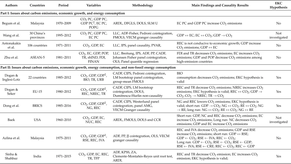
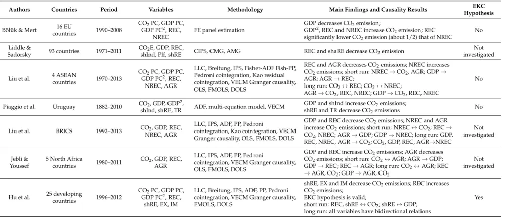
Recently, many studies have applied econometric approaches to investigate factors influencing CO2emissions (related studies are summarized in Table1, Table1in [11] also provides the related literature). The two most relevant strands of research are: (1) Examining the impacts of economic growth, energy consumption on carbon emissions. In this strand, the scholars mainly focused on two independent variables, namely the economic growth and energy consumption. These two variables are widely recognized to have impacts on carbon intensity and carbon emissions. Apart from the two common variables, different scholars would include other variables into their model according to their research objectives—e.g., Zhu et al. aimed to investigate the impacts of foreign direct investment (FDI) on CO2emissions, so Zhu et al. included FDI in their model [3]. (2) Analyzing the effects of economic growth and non-fossil energy consumption on carbon emissions. This strand originates from strand (1) because many scholars want to discover the impacts of renewable energy on CO2emissions. The main differences among these studies are the samples, the regression methods and the control variables. Therefore, we will analyze the existing literature from these two aspects.

2.1. Studies Examining the Impacts of Economic Growth and Energy Consumption on Carbon Emission There are plenty of studies concerning the relationship between CO2emission, economic growth and energy consumption, see details in Table1in [11]. The method and variables are similar in these studies; therefore, we select four recent studies here. There are three methodologies in these studies, namely OLS, panel VAR (PVAR), and panel quantile regression. To be specific, Begum et al. applied DOLS to investigate the relationship among carbon emissions, economic growth, and energy consumption in Malaysia, and concluded both energy consumption and economic growth raise carbon emissions [23]. Wang et al. used FMOLS to study the nexus in China from the provinces’ perspective, and concluded that both energy consumption and economic growth enhance carbon emissions. Moreover, there are bidirectional causal links between economic growth and energy consumption, and between energy consumption and carbon emissions, and there is a unidirectional causal link from economic growth to carbon emissions [21]. Antonakakis et al. employed PVAR to research the nexus from a panel of 106 countries, and concluded that economic growth increase CO2 emissions, and they also proved that there is a bidirectional causal link between economic growth and CO2emissions [24]. Zhu et al. applied panel quantile regression to study the nexus by using the data of five ASEAN countries, and discovered the impacts of the different determinants on CO2emissions shows a clear heterogeneity along with all quantiles [3].

(4)

Table 1.Summary of relevant studies on the two issues which are published between 2014 and 2018.

Authors Countries Period Variables Methodology Main Findings and Causality Results EKC

Hypothesis Part I: Issues about carbon emissions, economic growth, and energy consumption

Begum et al. Malaysia 1970–2009

CO2PC, GDP PC,

GDP PC2_{, EC PC,}

POPG

ARDL, DFGLS, DOLS, SLM U EC PC and GDP PC increase CO2emissions No

Wang et al. 30 China’s

provinces 1995–2012

CO₂PC, GDP PC, EC PC

LLC, ADF-Fisher, Pedroni cointegration,

FMOLS, VECM granger causality GDP↔EC; EC↔CO2; GDP→CO2

Not investigated Antonakakis

et al. 106 countries 1971–2011 CO2, GDP, EC LLC, IPS, panel causality, PVAR,

REC is not conducive to economic growth; GDP increase

CO2emissions; GDP↔EC No

Zhu et al. ASEAN-5 1981–2011

CO2, EC, GDP, POP,

TR, shIND, FDI, FINAN

LLC, Breitung, IPS, ADF, PP, CADF, Johansen Fisher panel cointegration, OLS, Panel quantile regression

FDI and TR decreases CO2emissions; EC increases CO2

emissions; GDP and POP decrease CO2emissions among

high-emission countries

No Part II: Issues about carbon emissions, economic growth, energy consumption, and non-fossil energy consumption

Dogan &

Inglesi-Lotz 22 countries 1985–2012

CO2, GDP, GDP2,

BIO, TR, URB

CADF, CIPS, Pedroni cointegration, LM bootstrap panel cointegration, group-mean FMOLS

BIO

consumption decreases CO2emissions; EKC hypothesis is

valid Yes Dogan & Seker EU-15 1980–2012 CO2, GDP, GDP2, REC, NREC, TR

CADF, CIPS, LM bootstrap cointegration, DOLS,

Dumitrescu-Hurlin non-causality

REC and TR decrease CO2emissions; NREC increases CO2

emissions; EKC hypothesis is valid; REC↔CO2; GDP→

CO2; CO2→NREC; TR→CO2

Yes

Dong et al. BRICS 1985–2016 CO2, GDP, GDP2, NG, REC

CADF, CIPS, Westerlund panel cointegration, panel AMG, VECM Granger causality

NG and REC lowers CO2emissions; EKC hypothesis is

valid; short run: GDP→CO2; NG↔CO2; RE↔CO2; NG →RE; long run: NG↔CO2; RE↔CO2; NG↔RE

Yes

Baek USA 1960–2010 CO2, GDP, EC,

NUC, REC ARDL, FMOLS, DOLS and CCR

Short run: GDP, NC and REC decrease CO2emissions; EC

increase CO2emissions; Long run: NC decreases CO2

emissions; GDP and EC increase CO2emissions

Not investigated

Azlina et al. Malaysia 1975–2011 CO2, GDP, GDP2, RSE, REC, IVA

ADF, PP, JJ cointegration, OLS, VECM granger causality

REC and IVA decrease CO2emissions; GDP and RSE

increase CO2emissions; short run: GDP↔RSE;

GDP←CO2; RSE←IVA; REC←CO2;

Long run: GDP←CO2; RSE←CO2; RSE←GDP;

RSE←IVA; RSE←CRE; REC←CO2; REC←GDP

No Sinha & Shahbaz India 1971–2015 CO2, GDP, EC, REC, TR, TFP ADF, KPSS, ZA,

Clemente-Montañés-Reyes unit root test, ARDL

REC and TR decrease CO2emission; EC increases CO2

(5)

Table 1.Cont.

Authors Countries Period Variables Methodology Main Findings and Causality Results EKC

Hypothesis Bölük & Mert 16 EU countries 1990–2008 CO2PC, GDP PC, GDP PC2_{, REC,} NREC FE panel estimation GDP decreases CO2emission;

GDP2_{, REC and NREC increase CO}

2emission; REC

significantly lower CO2emission (about 1/2) that of NREC

No Liddle &

Sadorsky 93 countries 1971–2011

CO2E, GDP, REC,

shInd, Pff, shRE CIPS, CMG, AMG REC and shaRE decrease CO2emission

Not investigated

Liu et al. 4 ASEAN

countries 1970–2013

CO2PC, GDP PC,

GDP PC2_{, REC,}

NREC, AGR

LLC, Breitung, IPS, Fisher-ADF Fish-PP, Pedroni cointegration, Kao residual cointegration, VECM Granger causality, OLS, FMOLS, DOLS

REC and AGR decreases CO2emissions; NREC increases

CO2emissions; short run: NREC→CO2, AGR; GDP→

AGR; AGR→REC;

long run: CO2↔REC; CO2↔NREC;

AGR→CO2, REC, NREC; GDP→CO2, REC, NREC

No

Piaggio et al. Uruguay 1882–2010 CO2, GDP, GDP2,

shInd, shRE, TR ADF, multi-equation model, VECM

GDP and shInd increase CO2emissions;

shRE and TR decrease CO2emissions No

Liu et al. BRICS 1992–2013 CO2, GDP, REC,

NREC, AGR

LLC, IPS, ADF, PP, Pedroni

cointegration, Kao cointegration, VECM Granger causality, OLS, FMOLS, DOLS

GDP and REC decrease CO2emissions; NREC and AGR

increase CO2emissions; short run: NREC↔CO2; REC→

CO2, NREC; AGR→GDP; GDP→NREC; long run: GDP,

REC, NREC, AGR→CO2; CO2, GDP, REC, AGR→NREC

Not investigated Jebli & Youssef 5 North Africa countries 1980–2011 CO2, GDP, REC, AGR

LLC, IPS, ADF, PP, Pedroni

cointegration, VECM Granger causality, OLS, FMOLS, DOLS

GDP and REC increase CO2emissions; AGR decreases

CO2emissions; short run: CO2↔AGR; AGR→GDP;

GDP→REC; REC→AGR; long run: CO2↔AGR; REC →AGR, CO2; GDP→AGR, CO2 Not investigated Hu et al. 25 developing countries 1996–2012 CO2PC, GDP PC, GDP PC2_{, REC,} shRE, EX, IM

LLC, Breitung, IPS, ADF, PP, Pedroni cointegration, VECM Granger causality, FMOLS, DOLS

shRE, EX and IM decrease CO2emissions; REC increases

CO2emissions;

EKC hypothesis is valid;

short run: REC, shRE↔CO2; shRE↔GDP;

long run: all variables have bidirectional relations

Yes

Note: (1) AGR (agricultural), CO2(CO2emission), CO2E (CO2emission from electricity production per capita), GDP (the gross domestic production), EC (energy consumption), EX (export),

BIO (biomass consumption), FDI (foreign direct investment), FINAN (financial development), IM (import), IVA (structural change in the economy), NUC (nuclear consumption), RSE (energy use in road sector), TR (trade openness), URB (Urbanization), Pff (price of fossil fuel), POP (population), POPG (population growth), PC (per capita), shRE (share of electricity production from non-fossil fuel sources), shInd (industry’s share of GDP), TFP (total factor productivity). (2) AMG (panel augmented mean group), ARDL (autoregressive distributed lag), ADF (augmented Dickey–Fuller unit root test), CADF (cross-sectionally augmented Dickey-Fuller unit root test), CIPS (cross-sectionally augmented Im, Pesaran, and Shin unit root test), CCR (canonical cointegration regression), CMG (common correlated effects mean group), DFGLS (Dickey–Fuller generalized least squared), DOLS (dynamic ordinary least squared), FE (fixed effect), IRF (impulse response functions), JJ (Johansen–Juselius co-integration tests), KPSS (Kwiatkowski–Phillips–Schimdt–Shin unit root test), LLC (Levin–Lin–Chu test), OLS (Ordinary Least Squares), PP (Phillips Perron unit root test), PVAR (panel vector autoregression), SLM U (Sasabuchi–Lind–Mehlum U test), VECM (vector error correction model), ZA (Zivot–Andrew unit root test).

(6)

2.2. Studies Examining the Influences of Economic Growth and Non-Fossil Energy Consumption on CO2Emissions

With regard to this issue, there are also many studies to research the interactions between carbon emissions, economic growth, and non-fossil energy consumption (see [10,11,18,19]). The method they used is similar, including OLS, FMOLS, DOLS, panel regression, and so on. However, the empirical results are not consistent with each other.

First, the non-fossil energy’s impacts on energy consumption are mixed. Although lots of scholars find non-fossil energy is useful for mitigating CO2emissions [8,9,11–14,17–20], but some scholars state an increase in renewable energy consumption increase CO2emissions [10,15,16]. Nevertheless, they find that non-fossil energy is still helpful for reduction of CO2emissions because renewable energy has significantly lower CO2emissions (about half) than non-renewable energy [10].

Second, the impacts of economic growth on carbon emissions are mixed. Dogan & Inglesi-Lotz, Dogan & Seker, Dong et al., Sinha & Shahbaz and Hu et al. proved the EKC hypothesis is valid [8,11,12,16,19]. However, Azlina et al. proved GDP has a linear relationship with CO2emissions in Malaysia [18], Bölük & Mert and Liu et al. proved inverted U-shaped is not applicable for EU and ASEAN [10,14].

Several reasons may explain the mixed results, like the data are different, the model and method used are different, and control variables are different [25]. However, we argue that the neglect of individual heterogeneity and distributional heterogeneity is the main reason for the different conclusions. As discussed above, most of existing literature applied common regression technique to investigating the influencing variables of CO2emissions, but they overlook the individual heterogeneity and distributional heterogeneity, which has been proven to have great influence on the regression results [3]. Therefore, in order to discover more details and to obtain more useful information about the influencing factors of CO2 emissions, we apply panel quantile regression technique in this paper, which constitutes an important contribution to the existing literature. Besides, unlike general studies, we use heating degree days and petroleum products in the transportation sector as explanatory variables for energy consumption, aiming to avoid the impacts of share data. Moreover, many studies neglect the competition relationship between non-fossil energy and fossil energy, so in order to find this relationship’s impact on CO2emission, we use crude oil price as a control variable. In short, compared with previous studies, especially [10,11] in which EU are analyzed, this paper has two contributions: (1) It applied panel quantile regression method, which may be more suitable than OLS method because both individual heterogeneity and distributional heterogeneity are considered. It can provide a complete picture of the relationship between the explanatory variables and CO2emissions. (2) Unlike previous studies, it used heating degree days and petroleum productions in the transportation sector as explanatory variables, rather than employed energy consumption as an independent variable. In this way, we can avoid a possible endogeneity problem.

3. Data and Method 3.1. Date

The data we use consist of panel data of carbon intensity of GDP (ton CO2/trillion€), GDP per Capita at 2010 market prices (€), gross electricity generation by nuclear and renewable (100 GWh), heating and cooling degree days, final consumption of petroleum products in transportation sector (kilo tonne of oil equivalent, ktoe), and Brent oil price in 28 European countries. The data are obtained from the European Commission. Our data covers the period from 1990 to 2015.

Carbon intensity of GDP (CDEI) is the dependent variable, and GDP per capita (GDPC), gross electricity generation by non-fossil energy (GEG), heating degree days (HDD), and petroleum products in the transportation sector (PPT) are the independent variables. The GDP per capita is measured in terms of 2010 market prices. To make patterns in the data more interpretable, we transform

(7)

the data into natural logarithms before empirical analysis. The specific definition of each variable is provided here:

(1) Carbon intensity of GDP is calculated as CO2emissions divided by GDP; it is measured as CO2emissions per unit GDP. Carbon intensity of GDP for different EU countries during 1990–2015 is illustrated in Figure1. For most of the EU countries, the carbon intensity of GDP decreases slightly over time (see details in Figure1), because most of them are developed countries. However, a minor increase in carbon intensity can be observed in some less-developed EU countries.

Sustainability 2018, 10, x FOR PEER REVIEW 7 of 20

transform the data into natural logarithms before empirical analysis. The specific definition of each variable is provided here:

(1) Carbon intensity of GDP is calculated as CO2 emissions divided by GDP; it is measured as

CO2 emissions per unit GDP. Carbon intensity of GDP for different EU countries during 1990–2015 is

illustrated in Figure 1. For most of the EU countries, the carbon intensity of GDP decreases slightly over time (see details in Figure 1), because most of them are developed countries. However, a minor increase in carbon intensity can be observed in some less-developed EU countries.

Figure 1. Carbon intensity of GDP in 28 European countries (after logarithm).

(2) GDP per capita at 2010 market prices equals to the gross domestic product divided by the population. The GDP per capita reflects the economic growth in one country and is considered a crucial factor for the carbon intensity in previous research [26,27]. Besides, other scholars also proved that economic growth affects carbon intensity by applying decoupling methods and convergence analysis [28–30]. GDP per capita for different EU countries during 1990–2015 is shown in Figure 2. We find an increasing trend in the GDP per capita for almost all EU countries by observing Figure 2. The trends for the carbon intensity of GDP and economic growth are opposite; this finding indicates that GDP may reduce the carbon intensity.

Figure 2. GDP per capita at 2010 market prices in 28 European countries (after logarithm).

Figure 1.Carbon intensity of GDP in 28 European countries (after logarithm).

(2) GDP per capita at 2010 market prices equals to the gross domestic product divided by the population. The GDP per capita reflects the economic growth in one country and is considered a crucial factor for the carbon intensity in previous research [26,27]. Besides, other scholars also proved that economic growth affects carbon intensity by applying decoupling methods and convergence analysis [28–30]. GDP per capita for different EU countries during 1990–2015 is shown in Figure2. We find an increasing trend in the GDP per capita for almost all EU countries by observing Figure2. The trends for the carbon intensity of GDP and economic growth are opposite; this finding indicates that GDP may reduce the carbon intensity.

transform the data into natural logarithms before empirical analysis. The specific definition of each variable is provided here:

(1) Carbon intensity of GDP is calculated as CO2 emissions divided by GDP; it is measured as

CO2 emissions per unit GDP. Carbon intensity of GDP for different EU countries during 1990–2015 is

illustrated in Figure 1. For most of the EU countries, the carbon intensity of GDP decreases slightly over time (see details in Figure 1), because most of them are developed countries. However, a minor increase in carbon intensity can be observed in some less-developed EU countries.

Figure 1. Carbon intensity of GDP in 28 European countries (after logarithm).

(2) GDP per capita at 2010 market prices equals to the gross domestic product divided by the population. The GDP per capita reflects the economic growth in one country and is considered a crucial factor for the carbon intensity in previous research [26,27]. Besides, other scholars also proved that economic growth affects carbon intensity by applying decoupling methods and convergence analysis [28–30]. GDP per capita for different EU countries during 1990–2015 is shown in Figure 2. We find an increasing trend in the GDP per capita for almost all EU countries by observing Figure 2. The trends for the carbon intensity of GDP and economic growth are opposite; this finding indicates that GDP may reduce the carbon intensity.

(8)

(3) Gross electricity generation by non-fossil energy is denoted by the gross electricity generated by nuclear and renewable energy. More precisely, renewable energy includes hydro energy, geothermal energy, solar energy, wind energy, and tide/wave/ocean energy. Figure 3describes different time series of gross electricity generation by non-fossil energy in EU countries. Overall, continued growth is observed in most EU countries. The trends for the carbon intensity of GDP and non-fossil energy are different, which implies that the use of non-fossil energy may decrease the carbon intensity of GDP.

(3) Gross electricity generation by non-fossil energy is denoted by the gross electricity generated by nuclear and renewable energy. More precisely, renewable energy includes hydro energy, geothermal energy, solar energy, wind energy, and tide/wave/ocean energy. Figure 3 describes different time series of gross electricity generation by non-fossil energy in EU countries. Overall, continued growth is observed in most EU countries. The trends for the carbon intensity of GDP and non-fossil energy are different, which implies that the use of non-fossil energy may decrease the carbon intensity of GDP.

Figure 3. Gross electricity generation by non-fossil energy in 28 European countries (after logarithm).

(4) Heating degree days are used to measure the energy demand which is incurred by heating buildings. To be specific, there is a benchmark temperature (such as 18° Celsius) below which the buildings need to be heated. Heating degree days refer to the accumulated degree which is below the benchmark temperature. Heating degree days are not only related to the location, but also related to incomes, building design, energy systems, and human behaviors. As we know, energy is consumed by industry use (including power generation), the transportation sector, and commercial/residential use. Heating degree days is a useful variable as it can reflect the activity of industry use and commercial/residential use. Figure 4 shows the time series of heating degree days in the EU countries. Overall, an intensive fluctuation is observed in most EU countries.

Figure 4. Heating degree days in 28 European countries (after logarithm).

Figure 3.Gross electricity generation by non-fossil energy in 28 European countries (after logarithm).

(4) Heating degree days are used to measure the energy demand which is incurred by heating buildings. To be specific, there is a benchmark temperature (such as 18◦Celsius) below which the buildings need to be heated. Heating degree days refer to the accumulated degree which is below the benchmark temperature. Heating degree days are not only related to the location, but also related to incomes, building design, energy systems, and human behaviors. As we know, energy is consumed by industry use (including power generation), the transportation sector, and commercial/residential use. Heating degree days is a useful variable as it can reflect the activity of industry use and commercial/residential use. Figure4shows the time series of heating degree days in the EU countries. Overall, an intensive fluctuation is observed in most EU countries.

(3) Gross electricity generation by non-fossil energy is denoted by the gross electricity generated by nuclear and renewable energy. More precisely, renewable energy includes hydro energy, geothermal energy, solar energy, wind energy, and tide/wave/ocean energy. Figure 3 describes different time series of gross electricity generation by non-fossil energy in EU countries. Overall, continued growth is observed in most EU countries. The trends for the carbon intensity of GDP and non-fossil energy are different, which implies that the use of non-fossil energy may decrease the carbon intensity of GDP.

Figure 3. Gross electricity generation by non-fossil energy in 28 European countries (after logarithm).

(4) Heating degree days are used to measure the energy demand which is incurred by heating buildings. To be specific, there is a benchmark temperature (such as 18° Celsius) below which the buildings need to be heated. Heating degree days refer to the accumulated degree which is below the benchmark temperature. Heating degree days are not only related to the location, but also related to incomes, building design, energy systems, and human behaviors. As we know, energy is consumed by industry use (including power generation), the transportation sector, and commercial/residential use. Heating degree days is a useful variable as it can reflect the activity of industry use and commercial/residential use. Figure 4 shows the time series of heating degree days in the EU countries. Overall, an intensive fluctuation is observed in most EU countries.

Figure 4. Heating degree days in 28 European countries (after logarithm). Figure 4.Heating degree days in 28 European countries (after logarithm).

(5) Petroleum products in the transportation sector are denoted by the total consumption of the LPG, motor gasoline and gas/diesel oil in the transportation sector of each country. It is used

(9)

to reflect the energy consumption in the transportation sector because most of the energy used in the transportation sector belongs to the products of crude oil. Figure5describes the time series of petroleum production in the transportation sector in EU countries. As we can see, there is a small fluctuation for most of the EU countries.

(5) Petroleum products in the transportation sector are denoted by the total consumption of the LPG, motor gasoline and gas/diesel oil in the transportation sector of each country. It is used to reflect the energy consumption in the transportation sector because most of the energy used in the transportation sector belongs to the products of crude oil. Figure 5 describes the time series of petroleum production in the transportation sector in EU countries. As we can see, there is a small fluctuation for most of the EU countries.

Figure 5. Petroleum products in the transportation sector in 28 European countries (after logarithm). Besides, we use Brent oil prices as a control variable, because there is a competition between fossil and non-fossil energy. Table 2 presents the descriptive statistics for all variables. As we can see in Table 2, the skewness and kurtosis values of all variables indicate that the six distributions have long tails, and are not normally distributed. Besides, the Jarque–Bera test clearly shows that all series depart from normality.

Table 2. Summary statistics (after logarithm).

Variables CEDI GDPC GEG HDD PPT Oil

Minimum 4.7131 7.8996 0.0000 5.8430 5.2364 2.5463 Maximum 8.1016 11.3530 8.5830 8.7661 11.1024 4.7152 Q1 (0.25) 5.7467 9.1933 3.6889 7.7672 7.4250 2.9611 Q3 (0.75) 6.5158 10.3124 6.1738 8.1621 9.1616 4.2828 Mean 6.2065 9.7196 4.7301 7.8751 8.4552 3.6133 STDEV 0.6244 0.7528 2.1478 0.5187 1.3920 0.7127 Skewness 0.6473 −0.3705 −0.6960 −1.5327 0.1400 0.2628 Kurtosis 0.0925 −0.6071 0.1065 2.6926 −0.5832 −1.4553 Jarque–Bera 51.362 *** 27.661 *** 59.424 *** 508.68 *** 12.471 *** 72.281 *** * significant at 10% level; ** significant at 5% level; *** significant at 1% level. 3.2. Panel Quantile Regression

In this study, a panel quantile regression model is used to analyze the effects of GDP per capita, gross electricity generation by non-fossil energy, heating degree days, petroleum products in the transportation sector, and Brent oil price on the carbon intensity of GDP in EU countries. By using this model, we can examine the driven factors of carbon intensity of GDP at different quantile levels. Much previous empirical research considered traditional conditional mean regression [26,31,32].

Figure 5.Petroleum products in the transportation sector in 28 European countries (after logarithm).

Besides, we use Brent oil prices as a control variable, because there is a competition between fossil and non-fossil energy. Table2presents the descriptive statistics for all variables. As we can see in Table2, the skewness and kurtosis values of all variables indicate that the six distributions have long tails, and are not normally distributed. Besides, the Jarque–Bera test clearly shows that all series depart from normality.

Table 2.Summary statistics (after logarithm).

Variables CEDI GDPC GEG HDD PPT Oil

Minimum 4.7131 7.8996 0.0000 5.8430 5.2364 2.5463 Maximum 8.1016 11.3530 8.5830 8.7661 11.1024 4.7152 Q1 (0.25) 5.7467 9.1933 3.6889 7.7672 7.4250 2.9611 Q3 (0.75) 6.5158 10.3124 6.1738 8.1621 9.1616 4.2828 Mean 6.2065 9.7196 4.7301 7.8751 8.4552 3.6133 STDEV 0.6244 0.7528 2.1478 0.5187 1.3920 0.7127 Skewness 0.6473 −0.3705 −0.6960 −1.5327 0.1400 0.2628 Kurtosis 0.0925 −0.6071 0.1065 2.6926 −0.5832 −1.4553 Jarque–Bera 51.362 *** 27.661 *** 59.424 *** 508.68 *** 12.471 *** 72.281 ***

* significant at 10% level; ** significant at 5% level; *** significant at 1% level.

3.2. Panel Quantile Regression

In this study, a panel quantile regression model is used to analyze the effects of GDP per capita, gross electricity generation by non-fossil energy, heating degree days, petroleum products in the transportation sector, and Brent oil price on the carbon intensity of GDP in EU countries. By using this model, we can examine the driven factors of carbon intensity of GDP at different quantile levels. Much previous empirical research considered traditional conditional mean regression [26,31,32]. However, this method may get the biased relevant coefficient or without finding important relationships [3,33]. In general, the interpretation of the conditional mean method is consistent with human intuition, and it is easy to calculate. In particular, if the error follows a normal distribution, the results of the least squares method are unbiased and efficient. However, in the area of risk

(10)

management, people often focus on the tail behavior of distributions. Meanwhile, the data usually is not normally distributed, with an apparent peak or fat tails. In this case, the results of the classic regression will get poor results. In addition, there often exist some abnormal points in the data, which will also affect the accuracy of the estimated results. Therefore, many scholars began to use quantile regression to avoid these issues mentioned above. Theτth quantile of a random variableYis

given by a quantile function:

QY(τ) =F_Y−1(τ) =inf{y:FY(y)≥τ} (1)

whereτ∈(0, 1)andFY(y) =P(Y≤y). This model captures the fact that the quantile functionQY(τ)

returns the minimum value ofyfrom amongst all those values whose cumulative distribution function (CDF) value exceedsτ.

The quantile regression, which was proposed by Koenker and Bassett Jr, has many advantages compared to the OLS regression [34], such as the empirical result of panel quantile regression is more robust [35], and there is no need to design distributional assumptions by using panel quantile regression [36]. Moreover, this method is able to capture the characteristics of the entire conditional distribution of all variables [37]. These are of particular interest in econometric analysis and forecasting (see [38–40], for example). The developments of quantile regression, as well as wide applications, has been summarized by Koenker and Hallock [41] and Yu et al. [42].

In order to take the impact effects and unobserved individual heterogeneity into consideration, we apply the model

QYi,t(τ|Xi,t) =α(τ) 0

Xi,t+βi, i=1, . . . ,N, t=1, . . . ,T (2) whereYi,tandXi,trepresent the carbon intensity and corresponding driven factors in countryiat time t, andβidenote the unobserved individual effects.α(τ)denote a vector of estimated parameters in the

equation, which are varying on different quantileτ. The main difficulties for solving Equation (2) is

that we cannot apply traditional linear approaches in the panel quantile regression model. To solve this problem, Koenker proposed an appropriate method with aL1-norm penalty term to eliminate unobserved fixed effects, called the shrinkage method [43]. This method is advantageous in controlling the variability caused by a lot of estimated individual coefficients and effectively reducing the number of estimated parameters. Here, we will apply this method to estimate our model, which is

argmin α K

∑

k=1 N

∑

i=1 T

∑

t=1 wkρτk n Yi,t−α(τ)0Xi,t−βi o +µ N

∑

i=1 |βi| i=1, . . . ,N, t=1, . . . ,T (3)

whereρτ(y) =y τ−1y<0is the traditional check function,1Ais the indicator function.iandtdenote the countries and the time, respectively.Kis the indicators for quantiles, andwk=1/Krepresent the relative weight on thek-th quantile, which is used to denote the contribution of different quantiles in this estimation (see [3,43]).µis the tuning parameter, it is used to determine the individual effect.

With reference to [3], we assume it is 1.

Furthermore, in this paper, we study the effects of GDP per capita, gross electricity generation by non-fossil energy, heating degree days, petroleum products in the transportation sector and Brent oil price on the carbon intensity of GDP in EU countries. In order to enable the specifications in our study to differentiate themselves from previous studies, we conduct our analysis by using the model

QYi,t(τ|Xi,t) =α1,τGDPCi,t+α2,τGEGi,t+α3,τHDDi,t+α4,τPPTi,t+α5,τOili,t+βi

i=1, . . . ,N, t=1, . . . ,T (4)

(11)

4. Empirical Findings and Analysis 4.1. Panel Unit Root Test

Before applying our model, we first adopt stationarity tests to verify which data we should use in our analysis, the selected level or the first difference. Such tests include Levin–Lin–Chu unit-root test [44], Fisher test [45], Hadri test [46], and modifiedp-test [47]. The tests results for six variables are listed in Table3. As we can see, the results indicate that all variables are stationary at 1% significant level. Therefore, we will use the selected level in the later empirical analysis.

Table 3.Panel unit root tests.

Variables CEDI GDPC GEG HDD PPT Oil

LLC −3.6437 *** −2.3534 *** −2.6079 *** −10.055 *** −12.691 *** −33.028 ***

Fisher 522.05 *** 336.85 *** 224.26 *** 724.56 *** 1503.4 *** 1606.3 ***

Hadri Test 78.491 *** 75.596 *** 57.479 *** 10.388 *** 50.714 *** 75.105 ***

Modifiedp-test 64.331 *** 15.054 *** 15.899 *** 43.621 *** 53.677 *** 114.19 ***

4.2. Panel Quantile Regression Results

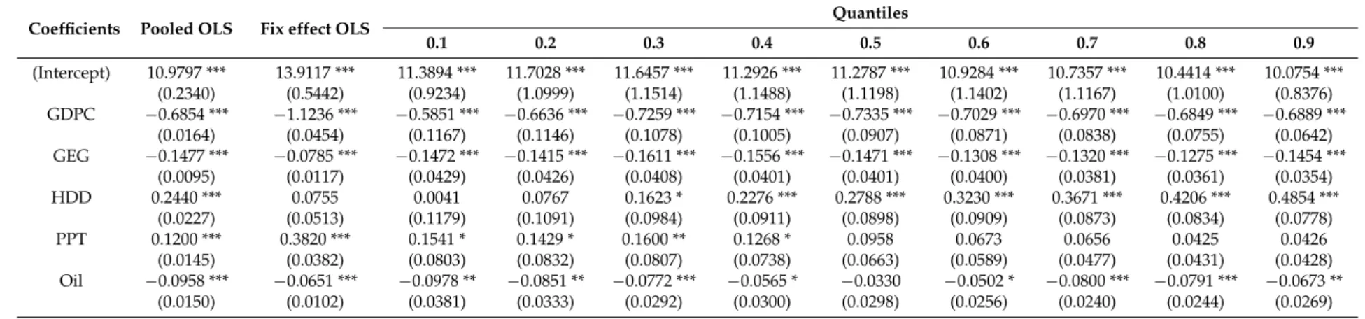
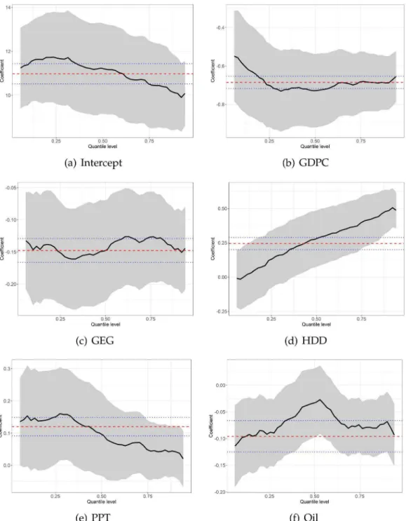
Our empirical results are listed in this section. In order to compare the regression results of OLS and panel quantile regression, the model is also estimated by using two panel OLS models, and the estimation results are presented in Column 1 and 2 in Table4. Other columns in Table4show the results of the estimation results of panel quantile regression with fixed effect at the different quantile levels. As shown in Table4, we conduct the panel quantile regression at intervals of 10th quantile of the conditional carbon intensity of GDP distribution. The estimation results in Table4clearly imply that the influences of different determinants on the carbon intensity of GDP are heterogeneous. The corresponding result is illustrated in Figure6, which allows us to observe the different change patterns of the coefficients of different variables with respect to different quantiles. In each subfigure of Figure6, thex-axis denotes the conditional quantiles of carbon intensity of GDP, and they-axis presents the coefficient values of different variables. Moreover, the black solid line shows the point estimation results at different quantile levels. The red dashed line represents the estimation results of the relevant OLS methods.

Firstly, we can observe that the impact of GDP per-capita is clearly heterogeneous and significantly asymmetric in Figure6b because the coefficients of different quantile levels change greatly with respect to different conditional distributional of carbon intensity of GDP. Overall, from a statistical perspective, the impact of GDPC is significant at 1% significance level and negative at all quantiles. To be specific, the coefficient initially decreases from−0.5851 at the 10th quantile to−0.7259 at the 30th quantile, and then slowly increases to−0.6889 at the 90th quantile. The negative coefficient means that an increase in GDP per capita will reduce the carbon intensity, which is reported in the earlier empirical study [10,11,27]. This finding implies that promotion of economic development may decrease carbon intensity. The main reason is that most EU countries are developed countries, and achieve a desired level of income. According to the EKC hypothesis, once the level of income exceeds the desired level (namely the turning point), the economic growth is useful to reduce carbon emissions. Moreover, the development policy of “inclusive and sustainable growth” is widely applied in the EU, which pays more attention to reducing carbon emissions. Overall, compared with OLS regression results, these results provide a complete picture about the influences of economic growth on CO2emissions, which provide support for our statement that OLS method overlooks the individual and distributional heterogeneity, and provide incomplete information about the impacts of economic growth on carbon intensity.

(12)

Secondly, Figure6c reveals that the impact of gross electricity generation by non-fossil energy on carbon emission intensity is also statistically significant and heterogeneous. There is significant asymmetry in the response of carbon intensity to gross electricity generation by non-fossil energy at different quantiles, which is similar to the impact of GDP per-capita. Overall, from a statistical perspective, the impact of GEG is significant at 1% significance level and negative at all quantiles. Specifically, the coefficient of GEG has a U-shaped curve trend at different quantiles, which initially decreases from−0.1427 at the 10th quantile to −0.1611 at the 30th quantile, and then increases to −0.1275 at the 80th quantile. The result indicates that the impact is less in the higher or lower quantiles of carbon emission intensity. The negative coefficient implies that an increase in non-fossil production will reduce the carbon intensity, which is also proven in [10,11]. This finding implies the promotion of non-fossil energy is helpful for the reduction of carbon intensity. Compared with fossil energy, non-fossil energy produces less CO2emissions in both the production and consumption process. Moreover, the estimation results prove that OLS regression can only present part of information about the impact of gross electricity generation by non-fossil energy on the carbon intensity of GDP.

Thirdly, the coefficient of heating degree days is insignificant at lower quantile levels of carbon intensity of GDP (specifically, the 10th and 20th quantile), but is significant at higher quantile levels (see Figure6d). Meanwhile, the coefficient of heating degree days is significant in pooled OLS mean regression. Therefore, OLS mean regression may bias the real coefficient, and it is not suitable to apply panel OLS method to investigate the impact of heating degree days on the carbon intensity of GDP. Overall, the coefficient of different quantile level increase from 0.0041 to 0.4854, indicating an apparent increasing trend with respect to the quantile levels of carbon intensity of GDP. The result indicates that when carbon intensity is relatively large, the carbon intensity may be significantly influenced by heating degree days. Compared with high carbon intensity countries, low carbon intensity countries are more developed. Correspondingly, the technology and residents’ consumption habits in low carbon intensity countries are better than the counterparts in high carbon intensity countries. High technologies are helpful to improve the thermal insulation performance of buildings and develop more sophisticated technology, such as ecological housing community or residential energy circulation system. Besides, residents’ good consumption habits can eliminate waste of energy. Therefore, the impacts of heating degree days on carbon intensity are more significant for medium and high quantiles.

Fourthly, as illustrated in Figure6e, the coefficient of petroleum products in the transportation sector on carbon intensity has a positive side but is insignificant at most quantile levels except for low quantiles (0.1, 0.2, 0.3, 0.4). To be specific, the impact is initially stable around 0.15 and then decrease from 0.1600 to 0.0426. However, the coefficient is significant in OLS panel data model at 5% significance level, implying that it is not suitable to apply OLS panel model to investigate the influence of petroleum products in the transportation sector on carbon emissions intensity of GDP. Overall, the coefficient is positively significant at low quantiles, but not significant in medium and high quantiles. This finding indicates that petroleum products in the transportation sector have more impact on carbon emission intensity when carbon emission intensity is relatively small. As the share energy use by transportation sector is small in the mix of total end-use energy in most of Europe countries, the share is about 31% in 2016 as reported in Exxon-Mobil’s 2018 outlook for energy. As for low carbon intensity EU countries, the percentage is even smaller than 31%. Besides, more non-fossil energy is used in the transportation sector in these countries. Therefore, an increase in petroleum products in the transportation sector may incur a substantial increase in carbon emissions, which in return raise the carbon intensity. This effect may not be that obvious for high carbon intensity EU countries because their energy use share of the transportation sector in total end-use is larger and they consume more fossil energy in the transportation sector.

(13)

Table 4.Panel quantile regression results.

Coefficients Pooled OLS Fix effect OLS Quantiles

0.1 0.2 0.3 0.4 0.5 0.6 0.7 0.8 0.9 (Intercept) 10.9797 *** 13.9117 *** 11.3894 *** 11.7028 *** 11.6457 *** 11.2926 *** 11.2787 *** 10.9284 *** 10.7357 *** 10.4414 *** 10.0754 *** (0.2340) (0.5442) (0.9234) (1.0999) (1.1514) (1.1488) (1.1198) (1.1402) (1.1167) (1.0100) (0.8376) GDPC −0.6854 *** −1.1236 *** −0.5851 *** −0.6636 *** −0.7259 *** −0.7154 *** −0.7335 *** −0.7029 *** −0.6970 *** −0.6849 *** −0.6889 *** (0.0164) (0.0454) (0.1167) (0.1146) (0.1078) (0.1005) (0.0907) (0.0871) (0.0838) (0.0755) (0.0642) GEG −0.1477 *** −0.0785 *** −0.1472 *** −0.1415 *** −0.1611 *** −0.1556 *** −0.1471 *** −0.1308 *** −0.1320 *** −0.1275 *** −0.1454 *** (0.0095) (0.0117) (0.0429) (0.0426) (0.0408) (0.0401) (0.0401) (0.0400) (0.0381) (0.0361) (0.0354) HDD 0.2440 *** 0.0755 0.0041 0.0767 0.1623 * 0.2276 *** 0.2788 *** 0.3230 *** 0.3671 *** 0.4206 *** 0.4854 *** (0.0227) (0.0513) (0.1179) (0.1091) (0.0984) (0.0911) (0.0898) (0.0909) (0.0873) (0.0834) (0.0778) PPT 0.1200 *** 0.3820 *** 0.1541 * 0.1429 * 0.1600 ** 0.1268 * 0.0958 0.0673 0.0656 0.0425 0.0426 (0.0145) (0.0382) (0.0803) (0.0832) (0.0807) (0.0738) (0.0663) (0.0589) (0.0477) (0.0431) (0.0428) Oil −0.0958 *** −0.0651 *** −0.0978 ** −0.0851 ** −0.0772 *** −0.0565 * −0.0330 −0.0502 * −0.0800 *** −0.0791 *** −0.0673 ** (0.0150) (0.0102) (0.0381) (0.0333) (0.0292) (0.0300) (0.0298) (0.0256) (0.0240) (0.0244) (0.0269)

(14)

Figure 6.Change in panel quantile regressions coefficients. Notes:y-axes show coefficient estimates

of named explanatory variable;x-axes depict the quantiles of the dependent variable. Shaded areas

correspond to 95% confidence intervals of quantile estimation. The red dashed line represents the estimation results of the relevant OLS methods, and the blue dashed line denotes the corresponding 95% confidence interval.

Fifthly, the coefficient of Brent crude oil price is insignificant and quite symmetric around its median, but significant at other quantiles (as shown in Figure6f). The impact of Brent crude oil price on carbon intensity has an inverted U-shaped curve trend, which increases from −0.0978 at the 10th quantile to−0.0330 at the 50th quantile and then decreases to−0.0800 at the 70th quantile. These results indicate that the Brent crude oil has a significantly negative influence on carbon emission intensity of GDP in both high and low carbon intensity countries. One possible explanation is that the

(15)

motivation of medium emission countries to reduce carbon intensity is not as strong as those of low and high emission countries. Therefore, they are not hurrying to cut down the use of fossil energy to change their consumption structure. Correspondingly, the impact of an increase of crude oil price is not very significant on their energy consumption structure, which in return has no significant impact on carbon intensity.

Finally, to verify the heterogeneity of the coefficients, we consider using Wald tests (see [48]) to compare the estimated coefficients of the 0.1 quantile and some higher quantiles (0.3, 0.5, 0.7, and 0.9 quantiles) and to verify whether they are significantly heterogeneous. Table5shows the results of the Wald test, which implies that the null hypothesis for GDP per capita, heating degree days and Brent oil price should be rejected, namely the effects of GDP per capita at 2010 market prices, heating degree days and Brent oil price on carbon dioxide emission intensity of GDP are not homogeneous at different quantiles. Therefore, it is important to consider the heterogeneous impacts of the influence factors on the carbon intensity of GDP at different quantile levels.

Table 5.Wald tests for the coefficient homogeneity (0.1 against 0.3, 0.5, 0.7, and 0.9 quantiles).

Against the 0.3 Quantile Against the 0.5 Quantile Against the 0.7 Quantile Against the 0.9 Quantile Test Statistic p-Value Test Statistic p-Value Test Statistic p-Value Test Statistic p-Value

GDPC 3.6786 * 0.0551 2.3302 0.1269 1.0462 0.3064 0.6719 0.4124

GEG 0.1699 0.6802 0.0000 0.9991 0.0892 0.7653 0.0010 0.9747

HDD 3.6914 * 0.0547 6.2669 ** 0.0123 8.9585 *** 0.0028 14.5115 *** 0.0001

PPT 0.0124 0.9114 0.7839 0.3759 1.3950 0.2376 1.6361 0.2009

Oil 0.3978 0.5283 2.7082 * 0.0998 0.2098 0.6469 0.5301 0.4666

To summarize, after comparing the estimation results of OLS and quantile panel data models, we can determine that fixed-effect panel quantile model provides a much richer and more comprehensive information of the effects of GDP per capita at 2010 market prices, gross electricity generation by non-fossil energy, heating degree days, petroleum products in transportation sector and Brent oil price on carbon intensity in the EU countries. In addition, these findings also help us to better understand the heterogeneity in the influence variables.

4.3. Robustness Check

To verify the robustness and the validity of our model, a robustness check which considers different values forµis conducted. To be specific, we assume thatµequals to 0.1, 0.9, and 2 respectively,

and conduct the panel quantile regression again. The estimation results for main variables are listed in Table6. As shown in Table6, the results for differentµbroadly conform to the main results in Table4.

In addition, we also perform two additional robustness checks by dropping variables. To be specific, we drop PPT and HDD respectively in the two additional robustness checks, and the corresponding results are listed in Tables7and8, respectively. As we can see, the estimation results for CDPC, GEG, and oil are roughly consistent with the results in Section4.2, which confirm the robustness of the results outlined in this paper.

(16)

Table 6.Robustness analysis: alternative values ofµ.

Coefficients Quantiles 0.1 0.2 0.3 0.4 0.5 0.6 0.7 0.8 0.9 µ= 0.1 GDPC −0.5851 *** −0.6636 *** −0.7259 *** −0.7154 *** −0.7335 *** −0.7029 *** −0.6970 *** −0.6849 *** −0.6889 *** (0.0000) (0.0000) (0.0000) (0.0000) (0.0000) (0.0000) (0.0000) (0.0000) (0.0000) GEG −0.1472 *** −0.1415 *** −0.1611 *** −0.1556 *** −0.1471 *** −0.1308 *** −0.1320 *** −0.1275 *** −0.1454 *** (0.0010) (0.0017) (0.0002) (0.0001) (0.0002) (0.0011) (0.0007) (0.0005) (0.0002) HDD 0.0041 0.0767 0.1623 0.2276 ** 0.2788 *** 0.3230 *** 0.3671 *** 0.4206 *** 0.4854 *** (0.9743) (0.5350) (0.1588) (0.0379) (0.0086) (0.0013) (0.0001) (0.0000) (0.0000) µ= 0.9 GDPC −0.5851 *** −0.6636 *** −0.7259 *** −0.7154 *** −0.7335 *** −0.7029 *** −0.6970 *** −0.6849 *** −0.6889 *** (0.0000) (0.0000) (0.0000) (0.0000) (0.0000) (0.0000) (0.0000) (0.0000) (0.0000) GEG −0.1472 *** −0.1415 *** −0.1611 *** −0.1556 *** −0.1471 *** −0.1308 *** −0.1320 *** −0.1275 *** −0.1454 *** (0.0009) (0.0011) (0.0003) (0.0005) (0.0013) (0.0028) (0.0024) (0.0021) (0.0006) HDD 0.0041 0.0767 0.1623 0.2276 * 0.2788 ** 0.3230 *** 0.3671 *** 0.4206 *** 0.4854 *** (0.9717) (0.5148) (0.1755) (0.0615) (0.0198) (0.0052) (0.0011) (0.0001) (0.0000) µ= 2 GDPC −0.5851 *** −0.6638 *** −0.7259 *** −0.7155 *** −0.7335 *** −0.7030 *** −0.6970 *** −0.6849 *** −0.6888 *** (0.0000) (0.0000) (0.0000) (0.0000) (0.0000) (0.0000) (0.0000) (0.0000) (0.0000) GEG −0.1471 *** −0.1416 *** −0.1611 *** −0.1556 *** −0.1471 *** −0.1307 *** −0.1319 *** −0.1275 *** −0.1454 *** (0.0008) (0.0009) (0.0001) (0.0000) (0.0000) (0.0001) (0.0002) (0.0004) (0.0001) HDD 0.0042 0.0768 0.1623 0.2275 ** 0.2789 *** 0.3230 *** 0.3670 *** 0.4205 *** 0.4854 *** (0.9710) (0.5033) (0.1328) (0.0270) (0.0029) (0.0003) (0.0000) (0.0000) (0.0000)

Note: Numbers in the parentheses representp-value. * significant at 10% level; ** significant at 5% level; *** significant at 1% level.

Table 7.Robustness analysis: excluding PPT.

Coefficients Quantiles 0.1 0.2 0.3 0.4 0.5 0.6 0.7 0.8 0.9 GDPC −0.5096 −0.5599 −0.6279 −0.6619 −0.6243 −0.6547 −0.6626 −0.6637 −0.6285 (0.0000) (0.0000) (0.0000) (0.0000) (0.0000) (0.0000) (0.0000) (0.0000) (0.0000) GEG −0.0536 −0.0665 −0.0759 −0.0882 −0.0998 −0.0922 −0.1002 −0.1072 −0.1234 (0.0031) (0.0020) (0.0023) (0.0008) (0.0002) (0.0007) (0.0002) (0.0001) (0.0000) HDD −0.0305 0.0365 0.1257 0.2210 0.2941 0.3223 0.3726 0.4185 0.4826 (0.6903) (0.7157) (0.2449) (0.0368) (0.0029) (0.0005) (0.0000) (0.0000) (0.0000) Oil −0.1414 −0.1282 −0.0851 −0.0708 −0.0652 −0.0708 −0.0702 −0.0748 −0.1055 (0.0000) (0.0000) (0.0203) (0.0464) (0.0493) (0.0181) (0.0100) (0.0051) (0.0002)

Note: Numbers in the parentheses representp-value. Table 8.Robustness analysis: excluding HDD.

Coefficients Quantiles 0.1 0.2 0.3 0.4 0.5 0.6 0.7 0.8 0.9 GDPC −0.5721 −0.6152 −0.6845 −0.7173 −0.7273 −0.7649 −0.7210 −0.6806 −0.6518 (0.0000) (0.0000) (0.0000) (0.0000) (0.0000) (0.0000) (0.0000) (0.0000) (0.0000) GEG −0.1493 −0.1259 −0.1218 −0.1121 −0.0945 −0.0731 −0.0647 −0.0864 −0.1112 (0.0001) (0.0018) (0.0048) (0.0143) (0.0592) (0.1737) (0.2193) (0.0819) (0.0163) PPT 0.1553 0.1232 0.1250 0.1343 0.1119 0.0785 0.0281 0.0074 −0.0065 (0.0294) (0.1274) (0.1553) (0.1356) (0.2199) (0.3758) (0.7296) (0.9161) (0.9101) Oil −0.0982 −0.1019 −0.1017 −0.0921 −0.0898 −0.0753 −0.1279 −0.1073 −0.1057 (0.0018) (0.0001) (0.0002) (0.0037) (0.0100) (0.0481) (0.0005) (0.0003) (0.0008)

Note: Numbers in the parentheses representp-value.

5. Conclusions and Suggestions

The key purpose of this paper is to research the influences of non-fossil energy, economic growth and energy consumption on the CO2intensity in EU 28 countries. In order to do so, we collect the annual samples of six variables from 1990 to 2015 of 28 EU countries. Considering that there are some limitations of OLS regression, and in order to find more useful information in limited data, we apply panel quantile regression method, which provides more details by taking unobserved individual heterogeneity and distributional heterogeneity into consideration. Moreover, in order to avoid the impact of shared data between CO2intensity and energy consumption, we use heating degree days and petroleum products in the transportation sector as explanatory variables in our model. Compared with

(17)

traditional OLS method, we think panel quantile regression method could discover more information by considering the impacts of various factors on CO2intensity at different quantiles.

5.1. Conclusions

(1) The regression results indicate that there exist heterogeneity and asymmetry effects at different quantiles with regards to the impacts of the determinants on carbon intensity. It implies that the panel regression method may be more suitable than OLS method because it can provide more details about the relationship between CO2emissions and the decisive factors, such as non-fossil energy, economic growth, heating degree days, and so on. It is meaningful for policy makers because the impacts of determinate variables are different for different countries. Therefore, policy makers could adjust their policies according to their own characteristics.

(2) The impact of non-fossil energy on carbon intensity is negative, which conforms to [9,11,13,14,17–19]. In particular, [11] also proved that non-fossil energy is helpful for the reduction of carbon emissions in EU countries by applying panel OLS method. However, our results indicate that the impact of non-fossil energy on carbon intensity is negative and significant at all quantiles, especially in the 0.3 quantile, which exhibits a U-shaped curve. It indicates that non-fossil energy is helpful for reduction of CO2emissions, but the impacts are different for different countries. Therefore, it proves that the traditional OLS regression method only provides the mean results, which is not the comprehensive relationship between variables and independent variables.

(3) As for economic growth, we find that economic growth has negative and significant impacts on carbon intensity, which is also proved in [10,13,20]. Particularly, [10] also demonstrated that economic growth mitigates CO2 emissions in EU countries. However, [10,13,20] applied the OLS method, which provided the same results for all countries. Nevertheless, we find that economic growth decreases carbon intensity, and its decreasing power is enhanced at medium and high quantiles.

(4) With regards to energy consumption, the effect of energy consumption is different for heating degree days and petroleum products consumption in transportation sectors: (1) the impact of heating degree days on carbon intensity is positive and becomes significant at higher quantiles. High carbon intensity countries are less developed; therefore, their technology and residents’ energy consumption habits may not be as good as low carbon intensity countries. Thus, heating degree days have a significant positive impact on high carbon intensity countries. (2) the effect of petroleum products consumption for the transportation sector is positive but not significant, except for low quantile. The energy consumption structure for low carbon intensity countries is cleaner than high carbon intensity countries; therefore, an increase in the petroleum products of the transportation sector has a more apparent impact for low carbon intensity countries.

(5) We find that the crude oil price’ impacts on carbon intensity present an inverted U-shaped curve with respect to different quantiles. The willing to reduce the carbon intensity of the medium carbon intensity countries may not be as strong as high and low carbon intensity countries; therefore, they are reluctant to change their energy consumption structure. Thus, the impact of an increase in crude oil price in medium carbon intensity countries is not as huge as the counterparts in high and low carbon intensity countries.

In summary, the contribution of this paper to the existing literature is that it applied the panel quantile regression method, and provide more details about the relationship between carton intensity and its decisive factors. Therefore, policy makers can make more suitable policies according to the countries’ own characteristics.

5.2. Suggestions

Based on the empirical results and our analysis, severval policy recommendations are proposed to further improve the environment in EU countries. (1) In terms of non-fossil energy, as non-fossil energy is helpful for the reduction of carbon intensity of GDP. Therefore, both high-carbon-intensity countries and low-carbon-intensity countries need to promote the development and consumption

(18)

of non-fossil energy, such as the government can encourage the application of renewable energy in the public sector. The city government in Baeza (Spain) has applied biomass energy to public lighting [49]. Moreover, the government can provide green finance to support the development of non-fossil energy [50]. (2) With regards to energy consumption, EU countries should further improve the energy efficiency in heating, use the more energy-saving material and apply circular economy in building sector, which will effectively reduce the energy consumption caused by heating demand [51]. EU countries also should reduce fossil fuel energy in the transportation sector, especially for low-carbon-intensity countries. This policy recommendation is consistent with the current EU policies as many EU government announced they would stop producing gasoline-fueled cars in the future. IPCC also suggests that improvement in energy efficiency and modification of energy structure are useful methods to mitigate carbon emissions [52]. (3) As for economic growth, our results suggest that medium-carbon-intensity and high-carbon-intensity countries would obtain a lot of benefits if their GDP per capita raised, compared with the counterparties of low-carbon-intensity countries. Therefore, medium-carbon-intensity and high-carbon-intensity countries should develop their economy. Nevertheless, the low-carbon-intensity countries should also try their best to promote their economy because economic growth in EU countries helps to reduce carbon intensity.

Author Contributions:Conceptualization, X.R. and C.C.; Methodology, X.R.; Software, X.R.; Validation, Z.W., X.R., and C.C.; Formal analysis, C.C.; Writing, X.R. and C.C.; Editing, Y.S.

Funding: This work is supported by the Young Fund of Shanxi University of Finance and Economics (no. QN-2018002), National Natural Science Foundation of China (no. 71774105) and Shanxi Repatriate Study Abroad Foundation (no. 2016-3).

Conflicts of Interest:The authors declare no conflict of interest.

References

1. United Nations.United Nations Framework Convention on Climate Change; United Nations: New York, NY,

USA, 1992.

2. The World Bank.World Bank Open Data; The World Bank: Washington, DC, USA, 2018.

3. Zhu, H.; Duan, L.; Guo, Y.; Yu, K. The effects of FDI, economic growth and energy consumption on carbon

emissions in ASEAN-5: Evidence from panel quantile regression.Econ. Model.2016,58, 237–248. [CrossRef]

4. Ozturk, I.; Acaravci, A. The long-run and causal analysis of energy, growth, openness and financial

development on carbon emissions in Turkey.Energy Econ.2013,36, 262–267. [CrossRef]

5. European Environment Agency.Progress towards 2008–2012 Kyoto Targets in Europe; Publications Office of the

European Union: Luxembourg, 2014.

6. Owusu, P.A.; Asumadu-Sarkodie, S. A review of renewable energy sources, sustainability issues and climate

change mitigation.Cogent Eng.2016,3, 1167990. [CrossRef]

7. International Energy Agency.CO2Emissions from Fuel Combustion 2017; International Energy Agency: Paris,

France, 2017.

8. Dogan, E.; Inglesi-Lotz, R. Analyzing the effects of real income and biomass energy consumption on carbon

dioxide (CO2) emissions: Empirical evidence from the panel of biomass-consuming countries.Energy2017,

138, 721–727. [CrossRef]

9. Liddle, B.; Sadorsky, P. How much does increasing non-fossil fuels in electricity generation reduce carbon

dioxide emissions?Appl. Energy2017,197, 212–221. [CrossRef]

10. Bölük, G.; Mert, M. Fossil & renewable energy consumption, GHGs (greenhouse gases) and economic

growth: Evidence from a panel of EU (European Union) countries.Energy2014,74, 439–446.

11. Dogan, E.; Seker, F. Determinants of CO2emissions in the European Union: The role of renewable and

non-renewable energy.Renew. Energy2016,94, 429–439. [CrossRef]

12. Dong, K.; Sun, R.; Hochman, G. Do natural gas and renewable energy consumption lead to less CO2

emission? Empirical evidence from a panel of BRICS countries.Energy2018,141, 1466–1478. [CrossRef] 13. Liu, X.; Zhang, S.; Bae, J.; Liu, X.; Zhang, S.; Bae, J. The nexus of renewable energy-agriculture-environment

(19)

14. Liu, X.; Zhang, S.; Bae, J. The impact of renewable energy and agriculture on carbon dioxide emissions:

Investigating the environmental Kuznets curve in four selected ASEAN countries.J. Clean. Prod.2017,164, 1239–1247. [CrossRef]

15. Jebli, M.B.; Youssef, S.B. The role of renewable energy and agriculture in reducing CO2 emissions:

Evidence for North Africa countries.Ecol. Indic.2017,74, 295–301. [CrossRef]

16. Hu, H.; Xie, N.; Fang, D.; Zhang, X. The role of renewable energy consumption and commercial services

trade in carbon dioxide reduction: Evidence from 25 developing countries.Appl. Energy2018,211, 1229–1244. [CrossRef]

17. Baek, J. Do nuclear and renewable energy improve the environment? Empirical evidence from the United

States.Ecol. Indic.2016,66, 352–356. [CrossRef]

18. Azlina, A.A.; Law, S.H.; Mustapha, N.H.N. Dynamic linkages among transport energy consumption,

income and CO2emission in Malaysia.Energy Policy2014,73, 598–606. [CrossRef]

19. Sinha, A.; Shahbaz, M. Estimation of Environmental Kuznets Curve for CO2emission: Role of renewable

energy generation in India.Renew. Energy2018,119, 703–711. [CrossRef]

20. Piaggio, M.; Padilla, E.; Román, C. The long-term relationship between CO2emissions and economic activity

in a small open economy: Uruguay 1882–2010.Energy Econ.2017,65, 271–282. [CrossRef]

21. Wang, S.; Zhou, C.; Li, G.; Feng, K. CO2, economic growth, and energy consumption in China’s provinces:

Investigating the spatiotemporal and econometric characteristics of China’s CO2emissions.Ecol. Indic.2016, 69, 184–195. [CrossRef]

22. Policies, Development and Current State of Non-Fossil Energy in European Union. Available online:

http://www.europarl.europa.eu/portal/en(accessed on 15 October 2018).

23. Begum, R.A.; Sohag, K.; Abdullah, S.M.S.; Jaafar, M. CO2emissions, energy consumption, economic and

population growth in Malaysia.Renew. Sustain. Energy Rev.2015,41, 594–601. [CrossRef]

24. Antonakakis, N.; Chatziantoniou, I.; Filis, G. Energy consumption, CO2emissions, and economic growth:

An ethical dilemma.Renew. Sustain. Energy Rev.2017,68, 808–824. [CrossRef]

25. Esteve, V.; Tamarit, C. Is there an environmental Kuznets curve for Spain? Fresh evidence from old data.

Econ. Model.2012,29, 2696–2703. [CrossRef]

26. Wang, P.; Wu, W.; Zhu, B.; Wei, Y. Examining the impact factors of energy-related CO2emissions using the

STIRPAT model in Guangdong Province, China.Appl. Energy2013,106, 65–71. [CrossRef]

27. Zhao, X.; Burnett, J.W.; Fletcher, J.J. Spatial analysis of China province-level CO2 emission intensity.

Renew. Sustain. Energy Rev.2014,33, 1–10. [CrossRef]

28. Roinioti, A.; Koroneos, C. The decomposition of CO2emissions from energy use in Greece before and during

the economic crisis and their decoupling from economic growth. Renew. Sustain. Energy Rev. 2017,76,

448–459. [CrossRef]

29. Villar Rubio, E.; Rubio, Q.; Manuel, J.; Molina Moreno, V. Convergence Analysis of Environmental Fiscal

Pressure across EU-15 Countries.Energy Environ.2015,26, 789–802. [CrossRef]

30. Wang, Q.; Zhao, M.; Li, R.; Su, M. Decomposition and decoupling analysis of carbon emissions from

economic growth: A comparative study of China and the United States.J. Clean. Prod.2018,197, 178–184.

[CrossRef]

31. Dietz, T.; Rosa, E.A. Effects of population and affluence on CO2emissions.Proc. Natl. Acad. Sci. USA1997, 94, 175. [CrossRef] [PubMed]

32. Fan, Y.; Liu, L.C.; Wu, G.; Wei, Y.M. Analyzing impact factors of CO2emissions using the STIRPAT model.

Environ. Impact Assess. Rev.2006,26, 377–395. [CrossRef]

33. Binder, M.; Coad, A. From Average Joe’s happiness to Miserable Jane and Cheerful John: Using quantile

regressions to analyze the full subjective well-being distribution.J. Econ. Behav. Organ.2011,79, 275–290. [CrossRef]

34. Koenker, R.; Bassett, G. Regression Quantiles.Econometrica1978,46, 33–50. [CrossRef]

35. Bera; Galvao, A.K.; Montes-Rojas, A.F.; Park, G.V.; Sung, Y. Asymmetric Laplace Regression: Maximum

Likelihood, Maximum Entropy and Quantile Regression.J. Econom. Methods2016,5, 79–101. [CrossRef]

36. Sherwood, B.; Wang, L. Partially linear additive quantile regression in ultra-high dimension.Ann. Stat.2016,

44, 288–317. [CrossRef]