Scott A. Sarra Marshall University Huntington, WV
A software suite written in the Java programming language for the postprocessing of Chebyshev approximations to discontinuous functions is presented. It is demonstrated how to use the package to remove the effects of the Gibbs-Wilbraham phenomenon from Chebyshev approximations of discontinuous functions. Additionally, the package is used to postprocess Chebyshev collocation and Chebyshev super spectral viscosity approximations of hyperbolic partial differential equations. The postprocessing method is the Gegenbauer reconstruction procedure. The Spectral Signal Processing Suite is the first publicly available package that implements the procedure. State of the art techniques are used to implement the algorithms with efficiency while reducing round-off error.
Categories and Subject Descriptors: G.1[Numerical Analysis] [G.1.2[Approximation]]: G.1.8[Partial Differential Equations]- spectral methods
General Terms: Algorithms
Additional Key Words and Phrases: Gegenbauer Postprocessing, Gibbs-Wilbraham Phenomenon, Java, Edge Detection, Chebyshev
1. INTRODUCTION
Spectral approximations based on Chebyshev polynomials are exponentially ac-curate for analytic functions. However, for discontinuous but piecewise analytic functions, the spectral partial sum approximates the function poorly throughout the domain. Away from the discontinuities, only first order accuracy is achieved. Near the discontinuity there areO(1) oscillations which do not decrease withN, the number of terms retained in the spectral partial sum. This is known as the Gibbs-Wilbraham phenomenon. The problem is reduced to one of signal processing in order to recover spectral accuracy.
Several methods exist for postprocessing spectral approximations. One class of postprocessing methods consists of variations of the spectral mollification (SM) idea which was originally developed in [Gottlieb and Tadmor 1985]. Spectral mollifica-tion involves applying a two parameter family of filters. The method can recover spectral accuracy up to within a neighborhood of each discontinuity. The Gibbs phenomenon can be removed, but some smearing at the discontinuity locations
Author’s address: S. Sarra, Department of Mathematics, Marshall University, One John Marshall Drive, Huntington, WV, 25755−2560. E-mail address: [email protected]
Permission to make digital/hard copy of all or part of this material without fee for personal or classroom use provided that the copies are not made or distributed for profit or commercial advantage, the ACM copyright/server notice, the title of the publication, and its date appear, and notice is given that copying is by permission of the ACM, Inc. To copy otherwise, to republish, to post on servers, or to redistribute to lists requires prior specific permission and/or a fee.
c
°20YY ACM 0098-3500/20YY/1200-0001 $5.00
will occur. This idea is discussed in more detail in [Kaber and Mahmoud 1994] and examples of using the method to postprocess PDE solutions are contained in [Kaber 1996]. The method of [Gottlieb and Tadmor 1985] can be improved upon if the locations of the edges are known [Gelb 2000; Tadmor and Tanner 2002]. This allows one of the two parameters to be optimized which leads to increased accuracy away from the discontinuities and less smearing at the discontinuities. Further opti-mization of the method is considered in [Tadmor and Tanner 2002]. While Spectral Mollification may be applied with or without the knowledge of the location of edges (discontinuities) in the function, better results are achieved when the locations of the edges are known.
Another way to postprocess spectral approximations is the Pad´e-based algorithm for removing the Gibbs phenomenon from Fourier approximations [Driscoll and Fornberg 2001]. The algorithm is stated in the context of Fourier approximations, but could possibly be extended to non-periodic Chebyshev approximations.
The postprocessing method that is the focus of the current version of the
Spec-tral Signal Processing Suite (SSPS) is the Gegenbauer Reconstruction Procedure
(GRP) [Gottlieb et al. 1992; Gottlieb and Shu 1997; 1996; 1995a; 1995b]. The GRP is capable of recovering spectral accuracy at every point, even at the locations of the discontinuities. However, despite showing more potential than Spectral Molli-fication, the GRP is not as robust as the SM postprocessing methods due to two un-optimized parameters used by the method. The GRP will need to know the location of edges in the function. The purpose of this paper and software package is to describe and implement the state of the art Gegenbauer Reconstruction Pro-cedure and Edge Detection algorithms. Prior to release 1.0 of the Spectral Signal Processing Suite, publicly available software that implemented the algorithms was not available.
The GRP may also be used to recover spectral accuracy from approximations of Partial Differential Equation (PDE) solutions arising from Chebyshev pseudospec-tral methods [Gottlieb and Shu 1995b]. In the context of postprocessing PDE solutions, the term edges refers to discontinuities and shocks. If the spectral approx-imation is to a nonlinear hyperbolic conservation law, spectral viscosity will need to be added to the approximation in order to obtain a stable approximation which converges to the exact entropy solution [Tadmor 1989]. While the spectral viscosity solution is a highly accurate approximation to the collocation solution, only partial theoretical justification can be found for using the postprocessing method on the spectral viscosity solution. Nevertheless, numerical results indicate that exponen-tial accuracy can be achieved by applying the Gegenbauer postprocessing procedure to the spectral viscosity solution [Gelb and Tadmor 2000b]. The same can be said about the edge detection method. The theoretical results are limited to locating the jump discontinuities of a piecewise smooth function, but numerical evidence advocates applying the edge detection procedure to the spectral viscosity solution. In the examples, we have used the Super Spectral Viscosity method (SSV) of [Ma 1998].
This paper is organized a follows. Section 2 reviews approximation by a Cheby-shev partial sum. Section 3 summarizes a method developed in [Gelb and Tadmor 2000a] to locate edges in a function. Section 4 summarizes the Gegenbauer
struction Procedure (GRP) postprocessing method. Section 5 describes the soft-ware suite. Section 6 presents examples of using the softsoft-ware suite to reconstruct piecewise analytic functions and examples of using the methods to postprocess the numerical solution of PDEs by Chebyshev pseudospectral methods. The numerical examples will emphasize both a local approach and a global approach for selecting the reconstruction parameters.
2. CHEBYSHEV APPROXIMATIONS
By a Chebyshev approximation of a function, we mean the Chebyshev partial sum
uN(x) = N X
n=0
anTn(x). (1)
The discrete Chebyshev coefficients,an, are defined by
an= 2 N 1 cn N X n=0 u(xj)Tn(xj) cj where cj= ½ 2 whenj= 0, N 1 otherwise. (2) The Chebyshev polynomials are known in closed form as
Tk(x) = cos(karccos (x)). (3) The Chebyshev pseudospectral method is based on assuming that an unknown PDE solution,u, can be represented by a global, interpolating, Chebyshev partial sum of the form (1). More detailed information on pseudospectral methods may be found in the standard references [Canuto et al. 1988; Fornberg 1996; Funaro 1992; Gottlieb and Orszag 1977; Gottlieb et al. 1984; Trefethen 2000].
If the PDE solution contains shocks, the Chebyshev pseudospectral method will not converge to the correct entropy solution [Tadmor 1989]. In this case, a spectrally small viscosity term must be added in order to stabilize the approximation and ensure convergence to the entropy solution. This can be done without sacrificing spectral accuracy and can be accomplished in several different ways, with each way being labelled a particular type of spectral viscosity method. In the examples, we have used the super spectral viscosity (SSV) method of [Ma 1998]. The reader is referred to [Sarra 2003a] for details on the implementation of the SSV method to the example problems.
3. EDGE DETECTION
If the exact location of discontinuities, or edges, in a piecewise analytic function are known, the Gegenbauer Reconstruction Procedure recovers spectral accuracy at all points, including the discontinuity points. If a PDE solution is being postprocessed and the solution contains rarefaction waves, discontinuities in the first derivative of the function will exist and will need to be located. The method used to find the edges originated in [Gelb and Tadmor 2000a] for periodic and non-periodic functions. The method is specialized to approximations of functions by Chebyshev methods and is summarized below.
Denote the location of discontinuities asαj.Let [f](x) :=f(x+)−f(x−) denote a local jump in the function and define
ue(x) = π √ 1−x2 N N X k=0 ak d dxTk(x) (4) where d dxTk(x) = ksin(karccos(x)) √ 1−x2 .
Essentially, we are looking at the derivative of the spectral projection of the nu-merical approximation to determine the location of the discontinuities. The series
ue(x) has the convergence properties
ue(x)→ ½ O¡1 N ¢ whenx6=αj [f] (αj) when x=αj.
The series converges to both the height and direction of the jump at the location of a discontinuity. However, the GRP does need the direction, it only needs the magnitude and location of the jumps. While a graphical examination of the series
ue(x) verifies that the series does have the desired convergence properties, an ad-ditional step is needed to numerically pinpoint the location of the discontinuities. For that purpose, make a non-linear enhancement to the edge series as
un(x) =NQ2[ue(x)]Q
The values, un(x), will serve to amplify the separation of scales which has taken place in (4). The series has the convergence properties
un(x)→ ( O ³ N−2Q ´ whenx6=αj NQ2 [[f] (αj)]Q whenx=αj.
By choosing Q > 1 we enhance the separation between the O([1
N]
Q
2) points of
smoothness and theO(NQ2) points of discontinuity. The parameterJ, whose value
will be problem dependent, is a critical threshold value. Finally, redefineue(x) as
ue(x) = ½
ue(x) ifun(x)> J
0 otherwise.
WithQlarge enough, one ends up with an edge detectorue(x) = 0 at all butO(1
N) neighborhoods of the discontinuities x = αj. Only those edges with amplitude larger thanJ1/Qp1/N will be detected.
Often the series ue is slow to converge in the area of a discontinuity and the nonlinear enhancement has a difficulty pinpointing the exact location of the edge. If an additional parameter,η, is added to the procedure this problem can be overcome in a simple manner. The parameter specifies that only one edge may be located in the interval (x[i−η], x[i+η]), i= 0, ..., N, with appropriate one sided intervals
being considered near boundaries. The correct edge will be the maximum ofuein this subinterval. The value of η is problem dependent and is best chosen after the edge detection procedure has been applied once.
The edge detection parametersJ,Q, andη, are all problem dependent. Various combinations of the parameters may be used to successfully locate edges represented by jumps of magnitude in a certain range.
As mentioned previously, if a PDE solution is being postprocessed and the so-lution contains rarefaction waves, the first derivative of the soso-lution will also have discontinuities and the edge detection procedure will have to be used to examine the first derivative of the solution in each piecewise smooth subinterval. After the shock locations are determined, the numerical solution can be differentiated in each
C0 smooth interval. Then, the locations of the discontinuities in the function and
its derivatives are arranged in increasing order.
In most situations, it is sufficient to consider a more na¨ıve approach which is easier to implement. If the numerical solution is differentiated over the entire computational domain, neighborhoods of noise will exist around the points where the edges in the solution were found. However, if the rarefaction waves are far enough away from the shock locations, edges in the derivative of the function can be successfully located by searching only a subinterval of the computational domain which is clear of any influence from the shocks.
4. GEGENBAUER RECONSTRUCTION PROCEDURE
The GRP works by expanding the function in another basis, theGibbs
complemen-tary basis, via knowledge of the known Chebyshev coefficients and the location of
discontinuities. The Chebyshev partial sums are projected onto a space spanned by the Gegenbauer polynomials. The approximation converges exponentially in the new basis even though it only converged very slowly in the original basis due to the Gibbs-Wilbraham phenomenon. The choice of a Gibbs complementary basis is the Ultraspherical or Gegenbauer polynomials,Cλ
n. The Gegenbauer polynomials are orthogonal polynomials of ordernwhich satisfy
Z 1 −1 (1−x2)λ−1/2Ckλ(x)Cnλ(x)dx= ½ hλ n k=n 0 k6=n where (forλ>0) hλ n =π 1 2Cnλ(1) Γ(λ+ 1 2) Γ(λ)(n+λ) with Cλ n(1) = Γ(n+ 2λ) n!Γ(2λ) .
Methods to implement the Gegenbauer Polynomials of degree (λ, m) are in the class
gegenbauerPolynomial of the SSPS.
The Gegenbauer expansion of a functionu(x), x∈[−1,1] is
u(x) = ∞ X l=0 b flλClλ(x)
where the continuous Gegenbauer coefficients,fbλ l, ofu(x) are b flλ= 1 hλ l Z 1 −1 ¡ 1−x2¢λ−1/2Clλ(x)u(x)dx (5) Since we do not know the functionu(x), implementing the GRP requires obtain-ing an exponentially accurate approximation, bgλ
l, to the first m coefficientsfblλ in the Gegenbauer expansion from the firstN+ 1 Chebyshev coefficients ofu(x). The approximate Gegenbauer coefficients are defined as the integral
b gλ l = 1 hλ l Z 1 −1 ¡ 1−x2¢λ−1/2Cλ l(x)uN(x)dx (6) where uN is the Chebyshev partial sum (1). The integral should be evaluated by Gauss-Lobatto quadrature in order to insure sufficient accuracy. The coefficientsgbλ l are now used in the Gegenbauer partial sum to approximate the original function as u(x)≈uλ m(x) = m X l=0 b gλ lClλ(x)
In practice, there will be discontinuities in the interval [−1,1] and the recon-struction must be done on each subinterval [a, b] in which the solution remains smooth. To accomplish the reconstruction on each subinterval, define a local vari-able for each subinterval asx(ξ) =²ξ+δ where ²= (b−a)/2,δ= (b+a)/2 and
ξj= cos(πj/N).The reconstruction in each subinterval is then accomplished by
uλ,² m(²ξ+δ) = m X l=0 b gλ ²(l)Clλ(ξ) where b g²λ(l) = 1 hλ l Z −1 1 (1−ξ2)λ−1/2Clλ(ξ)uN(²ξ+δ)dξ.
Notice that we have used collocation points on the entire interval [−1,1] to build the approximation in [a, b]. This is referred to as aglobal-local approach [Gottlieb and Shu 1995b]. The global-local approach seems to be best when postprocessing PDE solutions whereuN is obtained from the time evolution of the problem . The point values u(xi) may not be accurate, but the global interpolating polynomial
uN(x) is accurate.
In order to show that the GRP yields uniform exponential accuracy for the ap-proximation, it is necessary to select λ and m such that λ = m = β²N, where
β <2e/(27(1 + 1/2p)), andpis the distance from [−1,1] to the nearest singularity in the complex plane, in each subinterval where the function being reconstructed is assumed to be analytic [Gottlieb and Shu 1997]. The choice ofλ=mis neces-sary to make the proof work for the exponential convergence of the method, but in practice it is not necessary and usually not advisable to choose λ=m. We are often more concerned with obtaining results for a fixedN, rather than maintaining an exponential convergence rate.
If the function to be postprocessed consists of homogeneous features, the recon-struction parameters can be successfully chosen as λ=kλ²N andm =km²N for each subinterval wherekλandkmare user chosen, globally applied parameters. We refer to this strategy as the global approach. However, in problems with solutions containing varying detail throughout the computational domain, the reconstruction parameters may need to be chosen independently in each subinterval [Sarra 2002]. We refer to this strategy as thelocal approach. To date there is no known method to choose optimal values of the reconstruction parameters mandλ. The parameters remain very problem dependent.
4.1 Computational Expense
At first examination, the GRP seems to require a triple summation for each grid point value of a function that is reconstructed. The method can be very computa-tionally expensive asN andm grow. However, the use of the Christoffel-Darboux [Davis 1975] formula allows one of the sums to be eliminated [Gelb 2000]. The summation of the Chebyshev series can be done in an efficient manner with Clen-shaw’s recurrence formula [Clenshaw 1962]. These two modifications result in a much more efficient method and are implemented in the software.
4.2 Round-off Error
The Gegenbauer polynomials grow very rapidly with λ and m which leads to a round-off error that may completely ruin the approximation. Round-off error is especially problematic for functions with a lot of variation and that require large values ofmand/orλ. While the use of the Christoffel-Darboux formula reduces the computational effort, it adds to the round-off error problem as now two Gegenbauer polynomials are multiplied together. To lessen this problem Gelb [Gelb 2000] has suggested that the computation be rearranged in a way such that the two large and increasing Gegenbauer polynomial terms are first multiplied by quantities that are small and decreasing with respect to m,λ, andN. This rearrangement of the computation leads to a much more robust method and has been implemented in the software.
4.3 A Hybrid Approach
Even with the computational savings made via the Christoffel-Darboux formula, Gegenbauer Reconstruction may still be very computationally expensive in higher dimensions for large values ofN. A hybrid approach was suggested in [Gelb 2000] which uses an exponential filter, which may be applied very cheaply, in smooth regions and the GRP in the neighborhood of discontinuities. The exponential filter is σ(k N) = exp(−α| k N| β), (7)
whereαis the strength of the filter andβis the order of the filter. The exponential filter is an example of a spectral filter [Vandeven 1991] and can be used to recover a high order of accuracy away from points of discontinuity. The filtered partial sum takes the form
uN(x) = N X n=0 σ(n N)anTn(x)
Spectral filters do not completely remove the Gibbs-Wilbraham phenomenon, as oscillations in the neighborhood of discontinuities will not be removed.
The hybrid Gegenbauer postprocessing method is implemented for one-dimensional functions in the methodhybrid.postProcess().
5. SOFTWARE
Source code for the Spectral Signal Processing suite, a demonstration Applet con-taining all examples in this paper, and documentation of the graphical user interface (GUI) may be found atwww.scottsarra.org/signal/signal.html.
5.1 Supported Collocation Grids
The standard collocation points for a Chebyshev Collocation method are usually defined by
xj=−cos(πj
N), j= 0,1, ..., N. (8)
These points are extrema of the kth order Chebyshev polynomial Tk(x) (3). The points are often labelled the Chebyshev-Gauss-Lobatto (CGL) points, a name which alludes to the points role in certain quadrature formulas. The CGL points cluster quadratically around the endpoints and are less densely distributed in the interior of the domain. The CGL grid is denoted as grid 0 in the software. In practical ap-plication of Chebyshev Collocation methods for PDEs, a change of variable is often used to redistribute the collocation points. Three coordinate maps are supported by the software and are used in the examples.
The first map (grid 1 in the software) is the Kosloff/Tal-Ezer map [Kosloff and Tal-Ezer 1993]
x=g(ξ, γ) =arcsin(γξ)
arcsin(γ) , (9)
withγ∈(0,1). Asγapproaches one, the grid points become nearly evenly spaced and asγ approaches zero, the CGL grid is approached. The mapping also relaxes the O(N−2) time-stepping restriction that is present when advancing Chebyshev
methods with explicit time-stepping algorithms using the CGL grid. The second map (grid 2) [Basdevant et al. 1986] is
x=g(ξ, γ) = (1.0−γ)ξ3+γξ, (10)
with γ ∈ (0,1). Smaller values of γ cluster grid points around the center of the computational interval while still maintaining a dense grid point distribution near boundary points. As γ →1 the grid approaches the CGL grid. The map can be used to resolve regions of rapid variation in the center of a computational domain.
The two parameter tangent map (grid 3) [Bayliss and Turkel 1992] is
x=g(ξ, γ, µ) =x0+tan(δξ+ω)
γ (11)
whereκ= arctan(γ(1−µ)),γ= arctan(γ(1 +µ)),δ= 0.5(κ+γ),ω= 0.5(κ−γ), and x0 =−1 + 2(µ−a)/(b−a). The map can be used to resolve solutions with
either a region of rapid variation in the interior or at boundaries. The map can be used to cluster grid points around the pointµin the interval [a, b]. The parameter
γ >0 determines the degree to which the clustering takes place.
5.2 Summary of Signal Processing Classes
Two classes implement versions of the edge detection procedure. Both classes have one public method, findEdges. The findEdges method in class edgeDetect locates edges in a function on its entire domain. The method takes input: f, an array of function values, and edge detection parameters,J,Q, andη. The method outputs an array containing the edge series, ue, and nonlinear enhancement, nle. The location of the edges are returned in the Vectord. The Vector of edges can be used as input to the postprocessing methods.
edgeDetect.findEdges(double[] f, double J, int Q, double[] ue, double[] nle, Vector d, int eta)
The findEdges method in classedgeDetectAB is used to find edges in the derivative of a function in the interval [A, B]. The method is identical to the findEdges method in classedgeDetect except that it requires as additional input the endpoints of the interval searched as well as an array,xm, containing the grid on which the function
f is known.
edgeDetectAB.findEdges(double[] f, double J, int Q, double[] ue, double[] nle, Vector d, int eta, double A, double B, double[] xm)
Two versions of the Gegenbauer reconstruction procedure are implemented. Both classes implement one public method,postProcess. ThepostProcessmethod in class
gegenbauerReconstruction implements the procedure by using global reconstruction
parameters, LK and MK which are input into the method. The method also takes as inputs: an array of function values,f, and a vectord, containing the location of the edges. As output, the method returns an array, f G, containing the values of the postprocessed function. The methods also returns Vectorsmv andLv, which contain the value of the reconstruction parameters, m andλin each smooth sub-interval. The vectors mv andLv are used as input to the postProcess method of classgegenbauerReconstructionB.
gegenbauerReconstruction.postProcess(double f[], double d[], double LK, double MK, double fG[], Vector mv, Vector Lv)
ThepostProcessmethod of classgegenbauerReconstructionBimplements the local
approach to specifying reconstruction parameters.
gegenbauerReconstructionB.postProcess(double f[], double d[], double fG[], Vector mv, Vector Lv)
The methods takes as inputs: an array of function values, f, and a vector d, containing the location of the edges. Additionally, Vectors mv and Lv specifying the reconstruction parameters, m and λ, in each smooth subinterval need to be
input. The method returns the array f G containing the postprocessed function values.
The classeshybrid andhybridB implementpostProcess methods similar to those
of gegenbauerReconstruction and gegenbauerReconstructionB except that an
ex-ponential filter may be used to postprocess the input function in neighborhoods away from the edge locations. The methods in both classes take additional in-puts, alpha and gamma, which respectively determine the strength and order of the exponential filter (7). ThepostProcess method of class hybrid also takes as an input the parameterEP Swhich specifies that the GRP is to be applied in intervals (d[j]−EP S, d[j] +EP S) around each edged[j].
hybrid.postProcess(double f[], double d[], double LK,
double MK, double fG[], Vector mv, Vector Lv, double alpha, double gamma, double EPS)
ThepostProcess method of classhybridB allows different reconstruction
parame-ters to be applied in each smooth subinterval through the input VectorsmvandLv, in the same way that gegenbauerReconstructionB.postProcess does. Additionally, the value ofEP Saround each edge may be specified separately by values input in the Vectorev.
hybridB.postProcess(double f[], double d[], double fG[], Vector mv, Vector Lv, Vector ev, double alpha, double gamma) 6. EXAMPLES
The example functions are included as part of the software package and are avail-able from the examples menu in the GUI. The first four examples use the software suite to reconstruct functions approximated by a Chebyshev partial sum (1). The examples use two parameters,N ex, which sets the number of terms in the partial sum (1) toN ex+1, andM, which has various meanings depending on the example. The two parameters may be set through the GUI. The remaining examples demon-strate using the software as a postprocessing method for the Chebyshev Collocation method and Chebyshev SSV method. All PDE example problems can be stated as a system conservation laws with a source term as
ut+f(u)x=ψ(u). (12)
6.1 Step Function
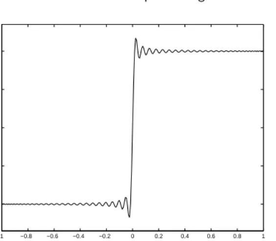
The first example consists of the step function on [−1,1] defined as f(x) = −1 if x 6 0 and f(x) = 1 if x > 0. The approximation of the step function by a Chebyshev series is shown in figure 1.
WithN ex= 60 and on the CGL grid (grid=0), the edge atx= 0, which has a jump of magnitude 2, can be located withJ = 10, Q= 1, andη = 2. This choice of edge detection parameters results in jumps ofJ1/Qp1/N≈0.9 and larger being located. In this case, we just need J1/Qp1/N > 0.85 to locate the correct edge location.
The function has a homogeneous structure throughout its domain, which indi-cates that the reconstruction parameters can be chosen globally. The reconstruction parameters can be specified by setting kλ = 0.1 and km = 0.025 which results in
−1 −0.8 −0.6 −0.4 −0.2 0 0.2 0.4 0.6 0.8 1 −1 −0.5 0 0.5 1
Fig. 1. step function approximation
m= 1 and L= 3 in each smooth subinterval. A slightly better result (check the error from the options menu) can be obtained withkλ= 0.5 andkm= 0.025 which results inm= 1 and L= 15 in each smooth subinterval.
6.2 Sine wave
The function f(x) = Sin(M πx) will test the resolution properties of the Gegen-bauer expansion. This smooth function contains M complete wavelengths in the interval [−1,1]. It was shown in [Gottlieb and Shu 1994] that the Gegenbauer expansions needs a minimum of π points per wavelength to completely resolve a wave.
ChooseN ex= 350, use the CGL grid (grid=0), and setM = 20. The function is smooth so there are no edges in the interval. If the global Gegenbauer parameters are set by specifying kλ = 0.003 and km = 0.25 (which results in m = 88 and
L= 1.05), the functions is well resolved.
6.3 Combination
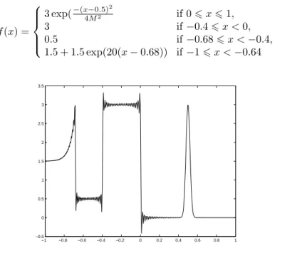
The previous two examples demonstrate that if the function has homogeneous struc-ture throughout its domain, then the reconstruction parameters can be chosen globally. However, if the function consists of subintervals of varying detail, a lo-cal approach to choosing the reconstruction parameters may be necessary. For example, consider function (13). Experimentally, we were unable to chose the re-construction parameters globally and obtain good results. Instead, a local approach seems necessary, where independent values of mand λare specified separately in each smooth subinterval.
For example, takeN ex= 400,grid= 0, andM = 0.015 to specify the width of the feature in the interval [0,1]. The edges can be located with J = 20, Q = 1, andη = 2. In the regions where the function is piecewise constant, reconstruction parameters of λ = 2 and m = 2 provide good results. In the region [−1,−0.68], the function is of moderate detail, and reconstruction can be accomplished with moderate values of m = 9 and λ = 9. In the interval [0,1], which consists of a narrow exponential spike, the function contains small scale structures which will
require a large value of m, and small value ofλ, similar to those in the Sine wave example, e.g.,λ= 0.1 andm= 70.
f(x) = 3 exp(−(x−4M02.5)2 if 06x61, 3 if−0.46x <0, 0.5 if−0.686x <−0.4, 1.5 + 1.5 exp(20(x−0.68)) if−16x <−0.64 (13) −1 −0.8 −0.6 −0.4 −0.2 0 0.2 0.4 0.6 0.8 1 −0.5 0 0.5 1 1.5 2 2.5 3 3.5
Fig. 2. Chebyshev Approx. of function (13)
6.4 Center Step
Theoretical proofs [Gottlieb and Shu 1995b] exist showing exponential convergence properties of the GRP for functions known on the CGL grid. Numerical evidence indicates that method may also be applied on grids arising from mappings of the Chebyshev grid. The determining factor in the accuracy of the reconstruction is how well the chosen grid can capture the function [Sarra 2002].
For example, consider the piecewise analytic function (14). Set N ex = 160,
M = 0.15, and form the grid with the map (9) with γ = 0.9999. The grid is nearly evenly spaced. The Chebyshev approximation of the function is shown in figure 14. The global Gegenbauer parameters can be set by specifyingkλ= 0.2 and
km = 0.025 to achieve a successful reconstruction of the function on the mapped grid.
f(x) = ½
0 ifx6M −1 orx>1−M ,
1 otherwise. (14)
6.5 Hyperbolic Heat Transfer
Our first example of using the GRP as a postprocessing method for Chebyshev Collocations method for PDEs is to the equations of hyperbolic heat transfer. The governing equations of hyperbolic heat transfer can be written in form (12) with
−1 −0.8 −0.6 −0.4 −0.2 0 0.2 0.4 0.6 0.8 1 0 0.2 0.4 0.6 0.8 1
Fig. 3. Chebyshev Approx. of function (14)
u= [T, Q]T,f(u) = [Q, T]T, ψ= [S/2,−2Q]T. T(x, t) is the temperature,Q(x, t) is the heat flux, and S(x, t) is the energy generation rate. Both examples used the initial conditionsT(x,0) = 0 andQ(x, t) = 0 on [0,1]. The problem is linear and the Chebyshev Collocation method is stable without the additional of any spectral viscosity. The system was advanced in time with a fourth order explicit Runge-Kutta method. More detailed information about the spectral solution of this problem may be found in [Sarra 2003b].
For the first hyperbolic heat transfer example, the system (12) is solved with boundary conditions ofQ(0, t) = 1,Q(1, t) = 0,Tt(0, t) =−Qx(0, t), andTx(1, t) = 0. The energy generation rate,S, set to zero.
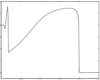
0 0.1 0.2 0.3 0.4 0.5 0.6 0.7 0.8 0.9 1 −0.2 0 0.2 0.4 0.6 0.8 1 1.2 1.4 1.6 1.8
Fig. 4. numerical (solid) vs. exact
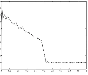
In the figure 4, the temperature solution,T, is shown at timet= 0.5 withN = 33
on the CGL grid (8). Strong oscillations are noticeable at the boundaryx= 0, due to the jump in the heat flux,Q,which is felt by the temperature.
0 0.1 0.2 0.3 0.4 0.5 0.6 0.7 0.8 0.9 1 −1 −0.5 0 0.5 1 1.5 2
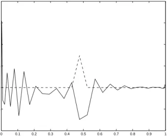
Fig. 5. edge series (solid) and enhancement
An edge is found to be atx= 0.476 with the parameters J = 200, Q= 4, and
η= 2. This choice of edge detection parameters results in jumps of 0.65 and larger being located. The exact jump is 0.65 in magnitude. By specifying η = 2, the oscillation nearx= 0 is not falsely determined to be a jump in the function. With only 33 grid points, the convergence of the edge series, figure 5, is not yet readily apparent. However, if the edge detection parameters are chosen appropriately, the correct edge locations will be found.
After the edges have been located, the GRP is applied in each smooth subinterval with by using global parameters chosen as kλ = 0.3 and km = 0.1 which results in m = 2 andλ= 4.7 in subinterval (0,0.476) and m= 2 and λ= 5.2 in subin-terval (0.476,1). For the homogeneous solution in this example, choosing global reconstruction parameters results in a successful application of the GRP.
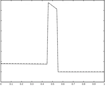
For the second hyperbolic heat transfer example, the system (12) is solved with solved with boundary conditions of Q(0, t) = 0, Q(1, t) = 0, Tx(0, t) = 0, and
Tx(1, t) = 0. The energy generation rate is specified asS(x, t) = 1
dn, if 0≤x≤dn, and zero otherwise. The energy generation rate, S, represents a pulsed energy source released instantaneously at timet= 0.
The temperature solution, (figure 7), with dn= 0.05 is shown at time t = 0.5 with N = 99 collocation points distributed with the map (9) with γ = 0.96. By taking the map parameter as γ = 0.96, the grid becomes closer to evenly spaced and better resolution is realized in the center of the domain.
Edges (figure 8) are found to be atx= 0.447 andx= 0.541 with the parameters
J = 5000, Q= 3, and N E= 1. With these choices of the edge detection parame-ters, only jumps of magnitude greater than 1.72 are found. Other combinations of
J andQcould work equally as well.
0 0.1 0.2 0.3 0.4 0.5 0.6 0.7 0.8 0.9 1 −0.2 0 0.2 0.4 0.6 0.8 1 1.2 1.4 1.6
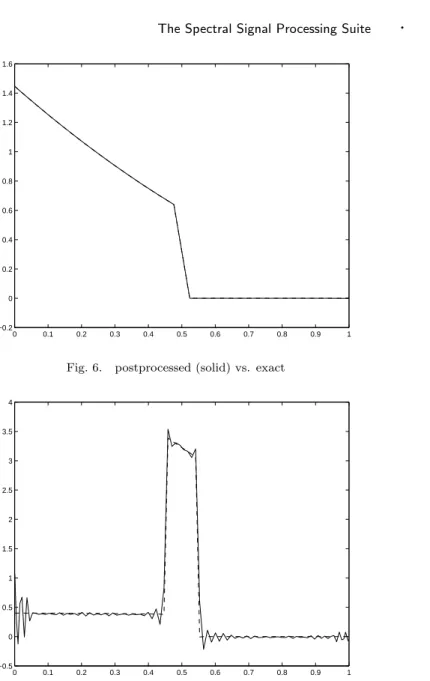
Fig. 6. postprocessed (solid) vs. exact
0 0.1 0.2 0.3 0.4 0.5 0.6 0.7 0.8 0.9 1 −0.5 0 0.5 1 1.5 2 2.5 3 3.5 4
Fig. 7. numerical (solid) and exact (dashed)
After the edges have been located, the GRP is applied in each smooth subinterval by using the global parameterskλ= 0.2 andkm= 0.02. The results are shown in figure 9.
6.6 Shallow Water Equations
Cast in the form (12), the Shallow Water Equations areu= [v, h]T,f(u) = [v2h+
0.5gh2, vh]T, and ψ(u) = 0. The variable h(x, t) is the height of the free upper surface,v(x, t) is the depth averaged fluid velocity, andgis the acceleration due to gravity.
0 0.1 0.2 0.3 0.4 0.5 0.6 0.7 0.8 0.9 1 −4 −3 −2 −1 0 1 2 3 4
Fig. 8. enhancement (solid) and edge series
0 0.1 0.2 0.3 0.4 0.5 0.6 0.7 0.8 0.9 1 −0.5 0 0.5 1 1.5 2 2.5 3 3.5
Fig. 9. postprocessed (solid) and exact
Our example is the dam break problem consisting of an initial condition of
h(x,0) = h0 if x < 0, h(x,0) = h1 if x > 0, and v(x,0) = 0. The solution
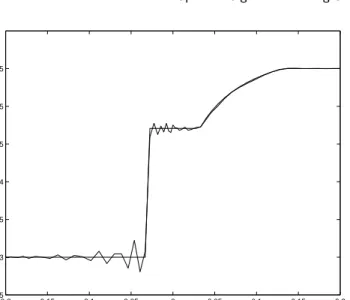
consists of a right moving shock and a left moving rarefaction. The Chebyshev SSV solution (figure 10) was calculated withN = 128 on a grid formed with map (9) withγ = 0.99. The system was advanced in time with a fourth order explicit Runge-Kutta method.
The edge detection procedure finds edges in the first derivative of the height solution in the interval [−1,0] atx=−0.475 andx=−0.374 with J= 70,Q= 2, andη = 1. A shock is found in the solution at x= 0.458 withJ = 1,Q= 1, and
−1 −0.8 −0.6 −0.4 −0.2 0 0.2 0.4 0.6 0.8 1 0.8 0.85 0.9 0.95 1 Fig. 10. SSV solution, h(x,t) η= 1.
The homogeneous features of the solution allow the reconstruction parameters to be chosen globally through the parameters kλ = 0.6 and km = 0.15. The postprocessed solution is shown in figure (figure 11).
−1 −0.8 −0.6 −0.4 −0.2 0 0.2 0.4 0.6 0.8 1 0.8 0.85 0.9 0.95 1 Fig. 11. postprocessed, h(x,t)
An exact solutions to the problem exists. However, for convenience, the refer-ence solution in the software was computed with the second order Nessayhu-Tadmor scheme [Nessyahu and Tadmor 1990] on a very fine grid (N = 4000) and interpo-lated with third order accuracy to the spectral grid.
6.7 Fluidized Bed Equations
Fluidized beds are used in the chemical and fossil fuel processing industries to mix particulate solids and fluids (gases or liquids). A typical fluidized bed consists of a vertically oriented chamber, a bed of particulate solids, and a fluid flow distributor at the bottom the chamber. The fluid flows upward through the particles creating a force that counteracts gravity at which time a state of minimum fluidization is reached. Stronger gas inflows (more than is necessary to maintain minimum fluidization) lead to pockets of gas, or equivalently low particle concentrations, resembling bubbles in a liquid travelling upward through the particles. Each rising bubble pushes a large amount of mass in front of it. Particles move downward through and around the rising bubble until it reaches the top of the bed. A settled bed is reestablished, and the cycle repeats. Each set of upward moving particles is referred to as a slug.
A model that represents a one dimensional simplification of two and three di-mensional fluidized bed models can be cast in the form on a nonlinear system of conservation laws in form (12) with u= [α, m]T and f(u) = [m, m2/α+F(α)]T. The variableα(x, t) denotes the concentration of particles by volume,m(x, t) =αv
represents the particle momentum, andv(x, t) the particle velocity.
A more detailed description of the model can be found in references [Christie et al. 1991] and [Christie and Palencia 1991]. If the source term is neglected, an exact solution to the Riemann problem for the homogeneous system can be found. The exact solution is developed in [Christie and Palencia 1991]. A detailed description of the Chebyshev SSV solution of the model may be found in [Sarra 2003a] and [Sarra 2002].
The appearance of the slugging behavior in the solution will create a solution with nonhomogeneous structure and detail throughout the domain of the problem. A local approach to specifying the reconstruction parameters will be needed.
6.7.1 Homogeneous System, shock-rarefaction. In our first example using the fluidized bed equations, we consider the Riemann problem for the homogeneous system for which an exact solution exists. This example consist of a left mov-ing shock and a right movmov-ing rarefaction wave. The initial conditions consist of
α(x,0) = 0.3 ifx <0 andα(x,0) = 0.55 ifx≥0. The initial velocity is v(x,0) = 0 for allx. The computation is done on a domain of [−0.2,0.2]. Figure 12 shows the SSV solution at t = 0.5. The grid consists of 64 points distributed by map (10) with γ= 0.25. The use of the coordinate map has the effect placing more points in the center of the domain. The system was advanced in time with a fourth order explicit Runge-Kutta method.
The rarefaction wave is characterized by the solution having a discontinuous first derivative, thus edge detection must be applied to the first derivative of the solution in addition to the solution itself. The edge detection procedure with Q = 1 and
J = 1 locates jumps of magnitude greater than 0.125. With these settings, the edge detection procedure locates edges in the function and the first derivative of the function atx=−0.0331,x= 0.0331, andx= 0.1374.
We were unable to get good postprocessed results by specifying the reconstruc-tion parameters globally through the parameters kλ and km. Global parameter specification failed due to the solution containing three intervals of piecewise
−0.2 −0.15 −0.1 −0.05 0 0.05 0.1 0.15 0.2 0.25 0.3 0.35 0.4 0.45 0.5 0.55
Fig. 12. α(x, t= 0.5), SSV approximation (oscillatory) vs. exact subinterval m λ
(-0.2,-0.033) 1 2 (-0.033,0.033) 1 3 (0.033,0.1374) 4 1 (0.1374,0.2) 1 2 Table I. local reconstruction parameters
stant values and a fourth interval, (0.033,0.1374), consisting of a function requiring different reconstruction parameters. Good results were obtained by specifying the GRP parameters locally in each smooth subinterval as listed in table I. The post-processed solution is shown in figure 13.
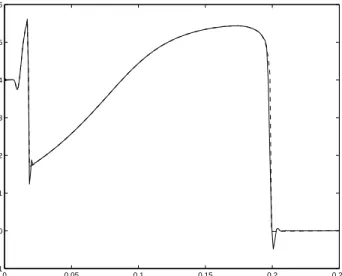
6.7.2 Slugging Problem. The initial conditions were taken as the state of mini-mum fluidization which is the state of the system at the minimini-mum gas flow necessary for the particle phase to be balanced by the upward force of the gas flow. Details of the exact determination of minimum fluidization for this problem may be found in [Sarra 2003a]. The non-homogeneous system was advanced in time with Strang splitting [Strang 1968] and a second order explicit Runge-Kutta method.
The SSV solution of the slugging problem is examined at t = 0.5, when the slugging behavior is first becoming apparent. The collocation grid consisted of 256 CGL (8) grid points. The edge detection procedure, figure 15, withJ = 1,Q= 1, and η = 2 located shocks at x = 0.01778 and x = 0.19822. The postprocessed solution, figure 14, was obtained by locally specifying the reconstruction parameters in each smooth subinterval as listed in table II.
An exact solution to the problem in not known. The reference solution included in the software was computed by Roe’s method [Roe 1981] with N = 1024 and interpolated with third order accuracy to the spectral grid. In figure 16, the Roe’s method solution is shown with the postprocessed spectral solution from figure 14.
−0.2 −0.15 −0.1 −0.05 0 0.05 0.1 0.15 0.2 0.25 0.3 0.35 0.4 0.45 0.5 0.55
Fig. 13. postprocessed (solid) vs. exact (dashed)
0 0.05 0.1 0.15 0.2 0.25 −0.1 0 0.1 0.2 0.3 0.4 0.5 0.6
Fig. 14. SSV (solid) vs. postprocessed, t=0.5 subinterval m λ
(0,0.01778) 15 2 (0.01778,0.19822) 14 4 (0.19822,0.25) 1 1 Table II. local reconstruction parameters
There is a good agreement between the two solutions. The slight variation in the two solution is largely due to the fact that Roe’s method is calculated on a uniform
0 0.05 0.1 0.15 0.2 0.25 −0.5 −0.4 −0.3 −0.2 −0.1 0 0.1 0.2 0.3 0.4 0.5
Fig. 15. edge series and enhancement(solid)
0 0.05 0.1 0.15 0.2 0.25 0 0.1 0.2 0.3 0.4 0.5 0.6
Fig. 16. postprocessed vs. reference (dashed), t=0.5
grid while the spectral method uses a nonuniform grid, which led to the initial conditions being slightly different. The solution of the system is very dependent on the initial conditions. The slightest variation of the initial conditions results in a noticeably different concentration profile at later times. A more detailed description of applying the GRP to this problem can be found in [Sarra 2003a] and [Sarra 2002].
7. CONCLUDING COMMENTS
In this paper, Version 1.0 of the Spectral Signal Processing Suite was described. In the current version methods are available to locate edges in and to postprocess
Chebyshev approximations of discontinuous functions. The algorithms have been implemented using the most efficient known methods, as a straight forward imple-mentation of the GRP algorithm is extremely costly. Additionally, steps have been taken to reduce round-off errors which plague the GRP algorithm.
Work is underway on version 2.0 of the SSPS. Version 2.0 will implement edge detection, the GRP, Spectral Mollification, Spectral Filtering, and Pad´e-based al-gorithms for both Chebyshev and Fourier approximations. SSPS 2.0 will contain a large number of the known methods that may be used to remove or reduce the Gibbs-Wilbraham phenomenon in spectral approximations of discontinuous func-tions. The package will allow the user to compare both the results and the efficiency of the various methods.
REFERENCES
Basdevant, C., Deville, M., Haldenvvang, P., Lacroix, J., Orlandi, D., Patera, A.,
Peyret, R.,and Quazzani, J.1986. Spectral and finite difference solutions of Burgers’ equa-tion. Comput. Fluids 14, 23–41.
Bayliss, A. and Turkel, E. 1992. Mappings and accuracy for Chebyshev pseudospectral ap-proximations.Journal of Computational Physics 101, 349–359.
Canuto, C.,Hussaini, M. Y.,Quarteroni, A.,and Zang, T. A. 1988. Spectral Methods for
Fluid Dynamics. Springer-Verlag, New York.
Christie, I.,Ganser, G.,and Sanz-Serna, J.1991. Numerical solution of a hyperbolic system of conservation laws with source term arising in a fluidized bed model.Journal of Computational
Physics 93,2, 297–311.
Christie, I. and Palencia, C.1991. An exact Riemann solver for a fluidized bed model. IMA
Journal of Numerical Analysis 11, 493–508.
Clenshaw, C.1962.Mathematical Tables, Volume 5. National Physics Laboratory, London.
Davis, P. J.1975.Interpolation and Approximation. Dover Publications, New York.
Driscoll, T. and Fornberg, B.2001. A Pad´e-based algorithm for overcoming the Gibbs phe-nomenon.Numerical Algorithms 26, 77–92.
Fornberg, B.1996.A Practical Guide to Pseudospectral Methods. Cambridge University Press, New York.
Funaro, D.1992. Polynomial Approximation of Differential Equations. Springer-Verlag, New York.
Gelb, A. 2000. A hybrid approach to spectral reconstruction of piecewise smooth functions.
Preprint.
Gelb, A. and Tadmor, E.2000a. Detection of edges in spectral data II: Nonlinear enhancement.
SIAM Journal of Numerical Analysis 38,4, 1389–1408.
Gelb, A. and Tadmor, E.2000b. Enhanced spectral viscosity approximations for conservation laws. Applied Numerical Mathematics 33, 3–21.
Gottlieb, D.,Hussaini, M. Y.,and Orszag, S. A.1984. Theory and application of spectral methods. InSpectral Methods for Partial Differential Equations, R. G. Voigt, D. Gottlieb, and M. Y. Hussaini, Eds. SIAM, Philadelphia, 1–54.
Gottlieb, D. and Orszag, S. A.1977.Numerical Analysis of Spectral Methods. SIAM, Philadel-phia, PA.
Gottlieb, D. and Shu, C.-W.1994. Resoulution properties of the Fourier method for discon-tinuous waves. Comput. Methods Appl. Mech. Engrg. 116, 27–37.
Gottlieb, D. and Shu, C.-W.1995a. On the Gibbs phenomenon IV: Recovering exponential accuracy in a subinterval from a Gegenbauer partial sum of a piecewise analytic function.
Mathematics of Computation 64, 1081–1095.
Gottlieb, D. and Shu, C.-W.1995b. On the Gibbs phenomenon V: Recovering exponential accu-racy from collocation point values of a piecewise analytic function.Numerische Mathematik 71, 511–526.
Gottlieb, D. and Shu, C.-W. 1996. On the Gibbs phenomenon III: Recovering exponential accuracy in a subinterval from a partial sum of a piecewise analytic function. SIAM Journal
of Numerical Analysis 33, 280–290.
Gottlieb, D. and Shu, C.-W. 1997. On the Gibbs phenomenon and its resolution. SIAM
Review 39,4, 644–668.
Gottlieb, D., Shu, C.-W.,Solomonoff, A.,and Vandeven, H. 1992. On the Gibbs phe-nomenon I: recovering exponential accuracy from the Fourier partial sum of a nonperiodic analytic function. Journal of Computational and Applied Mathematics 43, 81–98.
Gottlieb, D. and Tadmor, E.1985. Recovering pointwise values of discontinuous data within spectral accuracy. InProgress and Supercomputing in Computational Fluid Dynamics, E. M. Murman and S. S. Abarbanel, Eds. Birkh¨auser, Boston, 357–375.
Kaber, O. 1996. A Legendre pseudospectal viscosity method. Journal of Computational
Physics 128, 165–180.
Kaber, O. and Mahmoud, S. 1994. Filtering non-periodic function. Computer Methods in
Applied Mechanics and Engineering 116, 123–130.
Kosloff, R. and Tal-Ezer, H.1993. A modified Chebyshev pseudospectral method with an O(1/N) time step restriction. Journal of Computational Physics 104, 457–469.
Ma, H. 1998. Chebyshev-Legendre super spectral viscosity method for nonlinear conservation laws. SIAM J. Numer. Anal 35, 893–908.
Nessyahu, H. and Tadmor, E.1990. Non-oscillatory central differencing for hyperbolic conser-vation laws.Journal of Computational Physics 87, 408–463.
Roe, P.1981. Approximate Riemann solvers, parameter vectors, and difference schemes.Journal
of Computational Physics 43, 357–372.
Sarra, S. A.2002. Chebyshev pseudospectral methods for conservation laws with source terms and applications to multiphase flow. Ph.D. thesis, West Virginia University.
Sarra, S. A.2003a. Chebyshev super spectral viscosity method for a fluidized bed model. To
appear. Journal of Computation Physics.
Sarra, S. A.2003b. Spectral methods with postprocessing for numerical hyperbolic heat transfer.
To appear. Numerical Heat Transfer.
Strang, G.1968. On the construction and comparison of difference schemes. SIAM Journal of
Numerical Analysis 5,3, 506–517.
Tadmor, E. 1989. Convergence of spectral methods for nonlinear conservation laws. SIAM
Journal of Numerical Analysis 26, 30–44.
Tadmor, E. and Tanner, J.2002. Adaptive mollifers - high resolution recovery of piecewise smooth data from its spectral information. Foundations of Computational Mathematics 2, 155–189.
Trefethen, L. N.2000.Spectral Methods in Matlab. SIAM, Philadelphia.
Vandeven, H. 1991. Family of spectral filters for discontinuous problems. SIAM Journal of
Scientific Computing 6, 159–192.