Essays on Causal Inference with Endogeneity and Missing Data

(1)

DISCLAIMER:

This document does not meet

_the

current format guidelines

_of

the

Graduate School at

The University of Texas at Austin.

It has been published for

(2)

Copyright by Qian Feng

(3)

The Dissertation Committee for Qian Feng

certifies that this is the approved version of the following dissertation:

Essays on Causal Inference with Endogeneity and

Missing Data

Committee:

Stephen G. Donald, Supervisor

Jason Abrevaya

Haiqing Xu

(4)

Essays on Causal Inference with Endogeneity and

Missing Data

by

Qian Feng, B.Eco.; M.S. Econ.

DISSERTATION

Presented to the Faculty of the Graduate School of The University of Texas at Austin

in Partial Fulfillment of the Requirements

for the Degree of

DOCTOR OF PHILOSOPHY

THE UNIVERSITY OF TEXAS AT AUSTIN May 2017

(5)

Dedicated to my parents Liang Zhou and Zhenqi Feng, and to my husband Ryan Gu.

(6)

Acknowledgments

The first person I would like to thank is my supervisor, Stephen G. Donald, for his continuous support and guidance. Whenever I encounter dif-ficulties and obstacles in doing research, he is always able to point out the right direction and offer extremely helpful advice. I can’t forget the numerous fruitful and inspiring conversations I had with him. I wish I could grow into a successful scholar as him in the future and am so proud of being his student!

I would like to express my gratitude to Jason Abrevaya and Haiqing Xu. I not only learned great knowledge and receive help from them, but am also largely influenced by their working attitude and enthusiasm about research.

I want to thank everyone in our Econometrics Research Group at de-partment of Economics. I thank Sukjin Han, Brendan Kline, Jessie Coe, Xinchen Gu, Sungwon Lee, Peter Toth and Kaixi Wang. I benefit a lot from participating in the study group, writing seminars as well as lunch seminars and this is exactly where I was shaped into an econometrician.

I am grateful to my parents and my husband, who have provided me through moral and emotional support in my life. I can’t continue the journey towards a PhD without any of them. Special thanks to my husband Ryan Gu, who accompanies me getting over ups and downs and who is always ready to offer the unconditional love.

(7)

Essays on Causal Inference with Endogeneity and

Missing Data

Publication No.

Qian Feng, Ph.D.

The University of Texas at Austin, 2017

Supervisor: Stephen G. Donald

This dissertation strives to devise novel yet easy-to-implement estima-tion and inference procedures for economists to solve complicated real world problems. It provides by far the most optimal solutions in situations when sample selection is entangled with missing data problems and when treatment effects are heterogenous but instruments only have limited variations.

In the first chapter, we investigate the problem of missing instruments and create the generated instrument approach to address it. Specifically, When the missingness of instruments is endogenous, dropping observations can cause biased estimation. This chapter proposes a methodology which uses all the data to do instrumental variables (IV) estimation. The methodology provides consistent estimation with endogenous missingness of instruments. It firstly forms a generated instrument for every observation in the data sample that: a) for observations without instruments, the new instrument is an imputation;

(8)

b) for observations with instruments, the new instrument is an inverse propen-sity score weighted combination of the original instrument and an imputation. The estimation then proceeds by using the generated instruments. Asymp-totic theorems are established. The new estimator attains the semiparametric efficiency bound. It is also less biased compared to existing procedures in the simulations. As an illustrative example, we use the NLSYM data set in which IQ scores are partially missing, and demonstrate that by adopting the new methodology the return to education is larger and more precisely estimated compared to standard complete case methods.

In the second chapter, we provide Lasso-type of procedures for reduced form regression with many missing instruments. The methodology takes two steps. In the first step, we generate a rich instrument set from the many miss-ing instruments and other observed data. In the second step, IV estimation is conduced based on the generated instrument set. Specifically, the (very) many generated instruments are used to approximate a “pseudo” optimal instrument in the reduced form regression. The approach has been shown to have effi-ciency gains compared to the generated instrument estimator developed in the first chapter. We also compare the finite sample behavior of the new estima-tor with other Lasso estimaestima-tor and demonstrate the good performance of the proposed estimator in the Monte Carlo experiments.

The third chapter estimates individual treatment effects in a triangu-lar model with binary–valued endogenous treatments. This chapter is based on the previous joint work with Quang Vuong and Haiqing Xu. Following the

(9)

identification strategy established in (Vuong and Xu,forthcoming), we propose a two-stage estimation approach. First, we estimate the counterfactual out-come and hence the individual treatment effect (ITE) for every observational unit in the sample. Second, we estimate the density of individual treatment effects in the population. Our estimation method does not suffer from the ill-posed inverse problem associated with inverting a non–linear functional. Asymptotic properties of the proposed method are established. We study its finite sample properties in Monte Carlo experiments. We also illustrate our approach with an empirical application assessing the effects of 401(k) retire-ment programs on personal savings. Our results show that there exists a small but statistically significant proportion of individuals who experience negative effects, although the majority of ITEs is positive.

(10)

List of Tables

1.1 Summary Statistics for DGP1 . . . 32

1.2 Summary Statistics for DGP2 . . . 33

1.3 Rejection Rates: DGP2. . . 34

1.4 Checking for MCAR of IQ . . . 37

1.5 Instrumental Variables Estimation of Return to Education . . 38

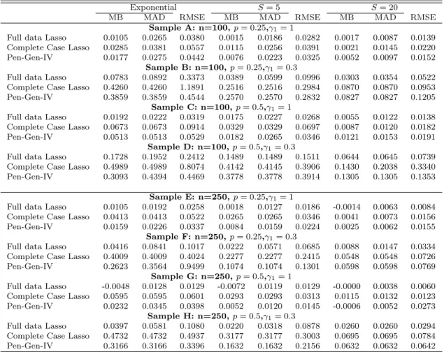
2.1 Summary Statistics for Many Missing instruments . . . 61

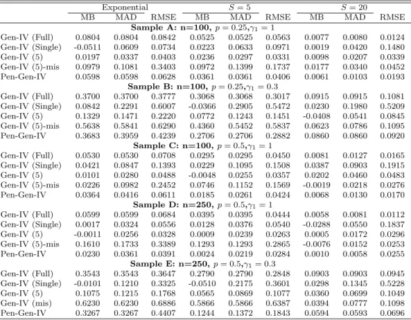
2.2 Comparison of Gen-IV and Pen-Gen-IV . . . 62

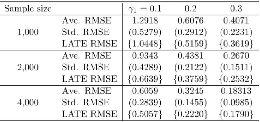
3.1 Finite sample performance of ITE . . . 77

3.2 Summary statistics . . . 86

3.3 Average FNFA (in thousand $) sorted according to covariates 87 3.4 OLS and 2SLS estimates of 401(k) participation . . . 88

3.5 Summary of ITE estimates (in thousand dollars) . . . 90

(14)

List of Figures

1.1 Distribution of the first-stage F statistic: DGP1 . . . 31

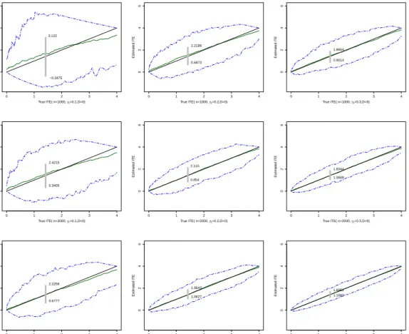
3.1 True and estimated ITE for D= 0 . . . 79

3.2 True and estimated ITE for D= 1 . . . 80

3.3 Estimated density of ITE. . . 81

3.4 Verifying the support condition . . . 89

3.5 The model restriction . . . 90

3.6 Estimated densities of ITE for full sample . . . 91

3.7 Estimated densities of ITE by income category . . . 92

3.8 Estimated densities of ITE by age category . . . 93

3.9 Estimated densities of ITE by family size category . . . 94

3.10 Estimated densities of ITE by marital status category . . . 94

3.11 Densities of potential outcome of nonparticipation . . . 96

(15)

Chapter 1 Instrumental Variable Estimation with

Missing Instruments

1.1 Introduction

Missing instruments occur in instrumental variables(IV) estimation when an instrumental variable has potentially missing values and is only available to a subsample of observations. For example, inAcemoglu and Robinson (2001), the mortality rate faced by early European settlers is used as an instrument for a country’s institutions, but the mortality rate is missing for about 56% of the sample1_{. However, the importance of missing instruments for} empiri-cal work has not been fully appreciated. Econometric literature has offered only a few solutions for addressing the problem. The most common proce-dure is simply dropping the observations with missing instruments in the IV estimation. When the missingness of instruments depends on the endogenous variable and/or other observed variables, existing solutions including dropping observations can result in biased and imprecise estimation.

In this chapter, I propose a methodology to deal with missing instru-ments. The methodology can provide consistent and less biased IV estimation

(16)

even when the missingness of instruments is endogenous. The main idea is to generate a new instrument, which is available to every observation in the data sample, to replace the original one with missing issues. I present a three-step estimation procedure. In the first step, a generated instrument is formed for every observation in the data sample. The generated instrument is an imputa-tion for individuals with missing instruments. The imputaimputa-tion is a predicted value for the missing instrument using completely observed variables. The generated instrument has a weighted combination form for individuals with observed instruments. The weight is the inverse propensity score, which is the probability of instrument being missing for the individual, after controlling for other completely observed variables. The combination is between the ob-served instrument and a predicted value of the instrument. The second and third steps are analogous to a standard two-stage least square (2SLS) proce-dure. The second step is a reduced form regression of the endogenous variable on the generated instrument and other exogenous variables. The third step is a structural estimation of the dependent variable on the fitted value of the endogenous variable and other exogenous variables.

Under certain regularity conditions, I am able to show that the new estimators is√n-consistent and asymptotically normal. My estimator belongs to the class of semiparametric doubly robust estimators (SDREs)2 in terms

2_{I follow the terminology of} _{Rothe and Firpo} ₍₂₀₁₃_{) and say that a semiparametric}

estimator based on doubly robust moment condition is SDRE if the moment condition depends on two unknown nuisance functions, but still identifies the parameter of interest if either one of these functions is replaced by some arbitrary value.

(17)

of that the generated IV is a Doubly Robust IV (DRIV). Even if one of the two nuisance parameters is misspecified, the DRIV remains valid. Another common feature shared by SDREs is that the required convergence rate for the nonparametric component is slower thann−1/4_{. I present explicit rate}

re-sults for sieve estimation of the nuisance functions and argue that compared to other two-step sieve estimation ((Chen, 2007), (Chen et al., 2008)), SDRE can have a richer choice of sieve spaces. In terms of efficiency, I first calculate semiparametric efficiency bounds under the model restrictions. Then I com-pare the asymptotic variances of my estimator to the efficiency bounds and prove that it attains the bounds under some conditions.

In the application, I revisit one empirical example of missing IQ scores fromCard (1995). I apply the new methodology for evaluating the return to education in which IQ score is an instrument for ability, which is proxied by the “Knowledge of the World of Work” (KWW) test score. the data set is the young men cohort from the National Longitudinal Survey 1976 (NLSYM76), in which IQ scores are missing about 30% of the sample. Card (1995) simply omits the observations with missing data in the IV estimation. I adjust the original IQ scores to generated IQ scores. Results show that by using generated IQ scores, return to education is increased from 8.9% to 13.9%, while the standard error reduces by 13%.

(18)

1.1.1 Related Literature

The methodology proposed in this chapter integrates ideas from the doubly robust (DR) estimation literature and the generated regressors liter-ature. My estimators are based on efficient moment conditions, which have the doubly robust property. This approach has precedent in literature on general missing data problems (e.g., (Robins et al., 1994), (Rotnitzky and Robins, 1995), (Scharfstein et al., 1999), (Van der Laan and Robins, 2003), (Bang and Robins,2005), (Wooldridge,2007), (Graham et al.,2012)). Recent studies focus on semiparametric versions of DR estimation. Rothe and Firpo

(2013) provides theoretical results for estimates derived from DR moment con-ditions. Belloni et al.(forthcoming) considers a semiparametric DR estimation for treatment effects. They estimate the first stage nuisance parameters using high dimensional machine learning methods. This chapter contributes to this line of research by developing efficient estimation procedure only through ad-justing the variable with missing values itself. In particular, I consider different treatments to observations with and without missing data, while maintaining the DR property of the estimator.

The new methodology is also related to semiparametric estimation us-ing generated regressors. Newey (2009) proposes a two-step series estimation of sample selection models, where the generated regressors from the first step are used to approximate the correction term. Theoretical results that charac-terize the influence of the generation step on the final estimator appear in e.g.

(19)

This chapter applies the methodology and techniques about generated regres-sors to the situation of generated instruments. I consider both parametric and nonparametric estimation in the second step using generated instruments formed in the first step.

This chapter differs from existing literature on missing instruments in two major aspects. First, I consider the endogenous missingness of instru-ments. Dahl and DellaVigna (2009) use a dummy variable approach to deal with missing value for an instrument. They enter a zero for the missing value and “compensates” by using dummies for “missingness”. Abrevaya and Don-ald (forthcoming) adds the interaction of dummy for missingness of other ex-ogenous variables to the instrument set of dummy variable approach and con-siders an efficient GMM estimator. However, these two approaches implicitly assume away the endogeneity issue of missing. They use a moment condition in which the error term is mean-independent of the instrument, within the subsample where the instrument is non-missing. Angrist et al.(2010) propose a full-sample instrument using a linear projection of the partially observed instrument on the covariates in the sub-sample with non-missing instrument.

Mogstad and Wiswall (2012) consider another full-sample instrument using instead a nonlinear projection, which is a nonparametric approximation to a conditional expectation. Neither of these two papers allows the dependence of missingness on the dependent variable, or the endogenous variable.

Second, the starting point of the methodology in this chapter is the efficient influence function under missing instruments. This chapter is then the

(20)

first to investigate efficient procedure to deal with missing instruments issue.

Chaudhuri and Guilkey (2013) illustrate the good finite sample performance of an augmented inverse propensity score weighted estimator when there are two missing instruments in the simulations. The chapter provides theoretical foundations for estimators based on efficient influence function and proposes an easy-to-implement procedure for execution.

1.1.2 Examples of Missing Instruments

Here I list several empirical examples in which instrumental variables have missing values, besides the aforementioned missing mortality rates (( Ace-moglu and Robinson, 2001)) and missing IQ scores ( (Card,1995)). The first example is the return to education. Some researchers use family background variables, e.g. parental education, as instrument for education ((Heckman and Li, 2004), (Flabbi et al., 2008) ,(Wang, 2013)). However, parental education is only available for individuals whose parents are present in the same house-hold3_{. The IVs are missing for the rest of the population whose parents are} living apart.

The second example is the quantity/quality model. The missing in-struments issue occurs in Angrist et al. (2010) when they combine different instrument sets across partially-overlapping parity-specific subsamples.

The last example is Mendelian Randomization4_. _{Recent studies in}

3_{Due to typical survey designs, information on parental characteristics is asked only when}

they are present in the same household.

(21)

health economics and epidemiology examine the causal effect of a risk fac-tor (e.g. obesity, early-childhood depression) on educational attainment. In

Smith and Hemani (2014), von Hinke Kessler Scholder et al. (2011), Kang et al.(2016), they use genetic variation as instruments. In one of the datasets they use, the Wisconsin Longitudinal Study (WLS), only 47% of the original sample have complete genetic data.

This chapter is organized as follows. Section 1.2 presents the IV model with missing instruments, the observational equivalence of the model with moment equations. Section 1.3 specifies the three-step procedure as well as the Gen-IV estimator. Section 1.4 establishes asymptotic results of the estimator. It also states the semiparametric efficiency bounds and discusses efficiency of the Gen-IV estimator. Section 1.5 provides simulation evidence of finite sample behavior of the estimators. Section 1.6 details the empirical application of return to education. Section 1.7 concludes the paper.

1.2 Model, Identification and the Generated Instrument

Consider the following standard linear regression model

Yi =Xiα+V

0

iβ+i, E(Vii) = 0, E(Xii)6= 0, i= 1, ..., n

Where Xi is an endogenous regressor and Vi is a dv-vector of exogenous

re-gressor. The first element of Vi is 1. There exists an instrumentZi which can

(22)

be (partially) missing. Zi satisfies

E(Zii) = 0 (1.1)

Let Di denote the missing indicator for Zi,

Di =

(

1, if Zi is missing

0, otherwise

For notational convenience, I In the following, I make distinction among

three cases of i.i.d. data samples. Thefull datasample consists of (Yi, Xi, Vi, Zi, Di)n_i₌₁,

which is the data sample we would want to collect on all the individuals

i = 1, ..., n. The observed data sample is (Yi, Xi, Vi,(1−Di)Zi, Di)n_i₌₁ which

is the actually observed data sample. The complete data sample consists of ((1−Di)Yi,(1−Di)Xi,(1−Di)Vi,(1−Di)Zi)n_i₌₁, which is the subsample of

data where the instrument Zi is observed for every individual5.

LetWi ≡(Yi, Xi, V

0

i)

0

, i.e. containing all the completely observed vari-ables. The missing indicator Di satisfies the “missing at random” (MAR)

assumption,

Assumption 1 (MAR). Di ⊥Zi|Wi

In the example of missing IQ scores, MAR indicates that the missing-ness of IQ scores doesn’t depend on the level of IQ scores, after conditioning on completely observed variables like wage, education and gender. In the missing

5_{One can instead write the complete data sample as (}_Y

i, Xi, Vi, Zi, Di) nc

i=1. ncis the

num-ber of individuals with complete data. This writing won’t change the estimation procedure proposed in this paper.

(23)

mortality rates example, MAR implies the propensity scores of missing mor-tality rates should be close for similar countries. Such kind of conditional inde-pendence assumption is also extensively used in econometrics and statistics to achieve identification with missing data. Examples include inference in models with attrition or nonresponse (e.g. (Little and Rubin,2014), (Robins and Rot-nitzky,1995), (Rotnitzky and Robins,1995), (Wooldridge,2002),(Wooldridge,

2007)), the estimation of treatment effects (e.g. (Heckman and Vytlacil,2007) and the references therein), the recovery of comparability over time of statistics calculated using data collected with different methodology.

Remark 1. MAR allows the dependence of missing indicatorDion completely

observed variable Wi. Consider the following example,

Di =1(%0+%1Yi+%2Xi+%3Vi ≤ui)

%0, %1, %2 and %3 are scaler constants, and ui is an error distributed by the

standard logistic distribution. Di depends on Yi, Xi and Vi as long as %1, %2,

%3 6= 0. ButDisatisfies MAR. I call the missingness endogenous if%21+%22+%23 6=

0.

The propensity score of Zi being missing is defined as the conditional

probability ofZi on the completely observed variable Wi,

p(Wi)≡P(Di = 1|Wi)

(24)

Assumption 2 (Overlap). 0≤p(Wi)<1−ν, for some ν >0.

This assumption effectively guarantees that, for any given valuew∈W, where W ⊂ Rdv+2 _{is the support of} _W

i, there is positive probability that the

instrument is observed. For large enough sample size n, there will be enough individuals with instruments near any point w for local methods to work.

Given Assumption1and Assumption2, the following lemma establishes an observational equivalence result between the IV model with single missing instrument and moment conditions. It is an extension to the equivalence result for a general missing data problem in Graham(2011).

Lemma 1 (Identification). Let Ze_i ≡(Z_i, V

0

i)

0

be the instrument set. The sin-gle missing instrument problem under Assumption 1 and 2 is observationally equivalent to the following moment restrictions.

E 1−Di 1−p(Wi) e Zii = 0 (1.2) E p(Wi)−Di 1−p(Wi) |Wi = 0 (1.3)

I follow terminology inGraham(2011) to call (1.2) the “identifying mo-ment” and (1.3) the “auxiliary moment”. The estimation method of inverse propensity score weighting (IPW) merely utilizes the identifying moment and regards the moment condition (1.3) as auxiliary since it only helps in estimat-ing the nuisance parameter p(Wi). See for example Hirano et al. (2003) for

reference. Doubly robust methods, however, adopt a certain combination of (1.2) and (1.3) for estimation. It is well known that a conditional moment

(25)

restriction is equivalent to infinite number of unconditional moment restric-tions6_{. Thus conditional moment (}_1.3_{) is equivalent to unconditional moment}

E p(Wi)−Di 1−p(Wi) g(Wi) = 0 (1.4)

for any measurable functiong(·)∈L2(W).

In the context of single missing instrument, I chooseg(Wi) = E(Ze_i|W_i)_i, wherei =i(Wi) = Yi−X∗

0

i θ, and consider the doubly robust, inverse

propen-sity score weighted combination of identifying moment (1.2) and unconditional moment (1.4). Specifically, the moment condition I am going to use for esti-mation is E 1−Di 1−p(Wi) e Zii− p(Wi)−Di 1−p(Wi) E(Zei|Wi)i = 0 =⇒E 1−Di 1−p(Wi)Zi− p(Wi)−Di 1−p(Wi) E(Zi|Wi) Vi ! i = 0 LetZi ≡ ₁−1−p(DWii)Zi− p(Wi)−Di

1−p(Wi) E(Zi|Wi). I callZi the generated instrument. As

a result, the actual instrument set used in estimation is Zei = (Zi, V

0

i)

0

. The following lemma shows that the generated instrumentZi is a valid IV.

Lemma 2(Validity of Generated IV). The generated instrumentZi is a valid,

full data instrument in terms of that it satisfies the excluded restriction.

E(Zii) = 0 (1.5)

where Zi = ₁₋1−_p₍D_Wi

i)Zi−

p(Wi)−Di

1−p(Wi) E(Zi|Wi).

6_{Several examples pointing out this equivalence include} _Bierens ₍₁₉₈₂_), _Chamberlain

(26)

Note that the generated IVZi contains two nuisance parametersp(Wi)

and E(Zi|Wi). The following corollary summarizes the Doubly Robust (DR)

property7 _of Z

i.

Corollary 1 (Doubly Robust IV). The generated IV Zi remains valid, i.e.

E(Zii) = 0 if either p(Wi) or E(Zi|Wi) is misspecified.

1.3 Estimation and the Gen-IV Estimator

Assume that the true value of the parameters of interest θ0 = (α0, β0)

0

lies in the interior of the compact parameter space Θ∈Rdv+1_{. The estimation}

is based on the sample analog of moment condition:

E(eZii) = 0 (1.6)

where Ze_i is the generated instrument set. I propose a three-step semipara-metric procedure for the estimation of θ based on (1.6). In the first step, the generated instrument Zi is estimated nonparametrically, denoted as bZ_i. The second step is a reduced form regression of the single endogenous variable Xi

on the generated instrument set b e

Zi = (bZi, V

0

i)

0

, which includes the estimated instrumentZb_i and other exogenous variablesV_i. The third step is a structural estimation of the dependent variableYion exogenous variableVi and the fitted

value Xb_i obtained in the second step. The following presents the estimation procedure in detail.

7_{A formal definition of DR is given in (}_{Bang and Robins}_, ₂₀₀₅_{): An estimator is DR}

if it remains consistent when either (but not necessarily both) a model for the missingness mechanism or a model for the distribution of the complete data is correctly specified.

(27)

Step 1 Estimation of generated instrument

The generated instrument Zi = ₁₋1−_p₍D_Wi_i₎Zi− p(Wi)

−Di

1−p(Wi) E(Zi|Wi) contains

two nuisance parameters which are the propensity score p(Wi) and the

con-ditional expectation E(Zi|Wi). Let h(Wi) ≡ E(Zi|Wi), hereafter. We first

estimate p(Wi) and h(Wi) nonparametrically and then form the generated

instrument by plugging in the nuisance estimates. In the following, I use sub-script cand m to refer to observations belonging to the complete data sample and subsample with missing instruments,respectively. Individuals in the the complete data sample are indexed by i = 1, ..., nc, while those in the missing

instrument sample are indexed byj = 1, ..., nm. It holdsn =nc+nm.

Assumption1implies that thefull data instrumentZi is mean

indepen-dent of the missing indicatorDi, controlling for completely observed variable

Wi,

h(Wi) =E(Zi|Wi) = E(Zi|Wi, Di = 0)

Hence we can use the complete data sample for the estimation of h(·). Let

{ql(w), l = 1,2, ...} be a sequence of known sieve basis functions, such as

power series, splines, Fourier series, etc. LetHdenote the sieve space spanned byql(w) H= ( h(w) =q(w)0π = ∞ X i=1 ql(w)πl )

A sieve least square estimator for h(w) is

bh(w) = nc X i=1 Zciqkh(n)(Wci)(Q 0 hQh)−1qkh(n)(w)

(28)

where qkh(n)₍_w_{) = (}_q 1(w), ..., qkh(n)(w)) 0 and Qh = (qkh(n)(Wc1), ..., qkh(n)(Wcnc)) 0

for some integerkh(n), withkh(n)→ ∞and kh(n)/n→0 when n→ ∞.

A sieve least square estimator for the propensity scorep(w), proposed inHahn (1998) is: b p(·) = arg min p(·)∈_Sn 1 n n X i=1 (Di−p(Wi))2/2 Sn =    s(w) = qkp(n)₍_w₎0_π ₌ kp(n) X j=1 qj(w)πj   

for some known basis (qj)∞j=1

whereSn is the sieve space spanned by the basis functions qj,j = 1, ..., kp(n).

The regularity conditions derived in this paper are based on the sieve esti-mation of the two nuisance functions. However, my estiesti-mation methodology doesn’t restrict the choice for estimation techniques to sieve only. One can use other nonparametric estimation, like kernel methods in obtainingp_b(·) andbh(·). In particular, machine learning methods, such as Lasso and random forests, are also suitable choices for estimating the two functions8_.

Furthermore, one can use parametric estimation for p_b(·) and bh(·) as well, which is potentially more appealing in empirical studies. h(Wi) can

8_{A valuable insight provided in}_{Belloni et al.}₍_forthcoming_{) is that, doubly robust moment}

conditions are key ingredients in deriving honest inference when machine learning methods are adopted for nuisance estimation

(29)

simply be a fitted value in a linear regression of instrument Zi on Wi in the

complete data sample:

bh(W_i) = W

0

iξb and p(Wi) can be parametrized as

p(Wi) =p(Wi;φ)

for a finite dimensional parameter φ. Estimates of φ can be obtained by maximizing

Πn_i₌₁{p(Wi;φ)}Di{1−p(Wi;φ)}1−Di

and _bp(Wi) =p(Wi;φb). Limited dependent variable estimation like Probit and Logit can execute the estimation well.

As a result, the generated instrument Zi is constructed by plugging in

b h(Wi) and pb(Wi), b Zi = 1−Di 1−p_b(Wi) Zi+ Di−pb(Wi) 1−p_b(Wi) b h(Wi) (1.7)

Note that in the subsample with missing instruments, the generated instru-ment is an impuation

b

Zmi=bh(Wmi)

On the other hand, in the complete data sample, the generated in-strument is an inverse propensity score weighted combination of the original instrumentZi and the estimated conditional expectationbh(Wi),

b Zci= 1 1−p_b(Wci) Zci− b p(Wci) 1−p_b(Wci) b h(Wci)

(30)

Step 2 Reduced form estimation

The reduced form estimator _bτ is an OLS estimator,

b τ = arg min τ∈B 1 n n X i=1 Xi−Zbe 0 iτ 2 = n X i=1 b e ZiZbe 0 i !−1 _n X i=1 b e ZiXi

where B ⊂Rdv+1 _{is a compact set, and} b e Zi = (Zb_i, V 0 i) 0 .

Step 3 Structural estimation

I define the Gen-IV estimator θb_GenIV as follows b θGenIV = (α,b βb) 0 = arg min θ∈Θ 1 n n X i=1 Yi−Xbiα−V 0 iβ 2 = n X i=1 b X_i∗X_i∗0 !−1 _n X i=1 b X_i∗Yi = n X i=1 b e ZiXi∗ 0 !−1 _n X i=1 b e ZiYi where Xbi =Zbe 0 iτband Xb ∗ i = (Xbi, V 0 i) 0 .

I leave the large sample properties of θb_GenIV to Section 4.

1.4 Asymptotic Results

(31)

1.4.1 Large Sample Properties of Gen-IV Estimator

For Gen-IV estimator, the asymptotic results established in this section is a generalization of the single missing instrument case. Namely, suppose now there is a fixed set of instruments Ai = A(Zi) ≡ (A1(Zi), A2(Zi), ..., At(Zi))

0

satisfying unconditional independence assumption E(Aii) = 0. The number

of instruments t doesn’t increase with the sample size n. And t is relatively small compared to the sample size, t << n.

I also allow the “structural” equation to have a general separable non-linear formYi =g(Xi∗;θ) +i. g(·) is a known function, which can be nonlinear

in Xi and/or Vi. In the single missing instrument case considered in Section

2, g(X_i∗;θ) =X_i∗0θ.

With fixed instrument set Ai, Step 2 and Step 3 in Section 2.2 are

now altered by a standard GMM procedure9 _{with estimated instrument set} b

Zi ≡ (bZi1, ...,Zb_it)

0

and weighting matrix G. The GMM version of Gen-IV estimator with fixed instrument set Ai is

b θGenIV = X∗0b e ZGbbeZ 0 X∗ −1 X∗0b e ZGbZbe 0 Y

in matrix notation, where ˆG is a consistent estimate of G, and b e Zi = (Zb_i, V 0 i) 0 .

9_{In the exact-identification case as in Section 2, the proposed three-step procedure}

coin-cides with a GMM procedure using generated instrument. The coincidence is analogous to that between a standard 2SLS and GMM.

(32)

1.4.1.1 Notation

Before listing regularity conditions, I first introduce some notations. Denote W ≡ X×Y×V = Rdv+2 ₌ _Rdw _{to be the support of the completely}

observed variablesWi = (Xi, Yi, Vi), and W is allowed to be unbounded. For

any 1×dw vectora= (a1, ..., adw) of nonnegative integers, write|a|=

Pdw

i=1ai.

Denote the |a|th derivative of a function l :W→R as

Oal(w) = ∂ |a| ∂wa1 1 · · ·∂w adw dw l(w)

The Hölder space Λγ(W) is a space of functions with up to [γ] continuous derivatives10, and the highest (γth) derivatives are Hölder continuous with the Hölder exponentγ−[γ]∈[0,1). The Hölder space is endowed with the norm

||l||Λγ = sup w |l(w)|+ max |a|=[γ]_wsup6= ¯w |_O|a|_l₍_w₎₋ O|a|l( ¯w)| p (w−w¯)0(w−w¯)γ−[γ] A H¨older ball Λγ

c(W) with radius cis defined as

Λγ_c(W) = {l ∈Λγ(W) :||l||Λγ ≤c <∞}

Define a weighted sup-norm ||l||∞η ≡ supw∈_W|l(w)(1 + ||w||2)−

η

2| for some

η >0. The role [1 +|w|2_]−η·/2 _{plays is similar to that of a trimming procedure}

in Kernel methods, where smaller weight is imposed upon larger values of

W. Denote Π∞nl to be the projection of l onto the sieve space Sn under

the norm || · ||∞η. A weighted H¨older ball Λγc(W, η) with radius c is then

Λγ

c(W, η)≡ {l ∈Λγ(W) :||l||∞η ≤c <∞}.

(33)

The two nuisance functionsp(·) andh(·) belong to H¨older spaces Λγp₍W₎

and Λγh₍W_{). The weighted sup-norms for the two spaces are} || · ||

∞ηp and

|| · ||∞ηh, respectively. To avoid tedious notation, I just let γ = γp = γh, and

η=ηp =ηh.

1.4.1.2 Consistency

The regularity conditions in the following assumption are required for the consistency of Gen-IV estimator.

Assumption 3. Let Gb−G=o_p(1) for a positive semidefinite matrix G, and the Jacobian Jθ ≡ −_∂θ∂ E[Ze_ig(X_i∗;θ)], the following hold

(3.1) Jθ0 has full column rank equal to dv+ 1.

(3.2) p0(·) belongs to H¨older ball S= {p(·) ∈Λγc(W, η) : 0 < p ≤p(w) ≤p <¯

1,∀w∈W}, h0(·) is H(γ, η1)-smooth for some η1 ≥0.11

(3.3) E((1 +||Wi||2) η )<∞ for some η > η1 ≥0. (3.4) (i) E(||A(Zi)i||2)<∞, E(||h0(Wi)i||2)<∞, σ2 ≡E(2i)<∞. (ii)E(||A(Zi)i||(1+||Wi||2) η 2)<∞,E(||A(Z_i)||2)<∞, E(||h₀(W_i)||2)< ∞.

(34)

(3.5) There is a function b(·) s.t. b(δ)→0 as δ →0 and E sup ||θ−_θ˜||<δ |g(X_i∗;θ)−g(X_i∗; ˜θ)|2 ! ≤ b2(δ) E sup ||θ−_θ˜||<δ |(Yi−g(Xi∗; ˜θ))(1 +||Wi||2) η 2| ! ≤ δ

for a small positive value δ.

(3.6) For any function l1 ∈ S, and any l2 ∈ Λcγ(W.η), there are Π∞nl1 and

Π∞nl2 in the sieve spaces Sn and Hn such that

||l1−Π∞nl1|| = op(1)

||l2−Π∞nl2|| = op(1).

Also E[qkh(n)₍_W₎0_qkh(n)₍_W_)] _{is non-singular uniformly in} _k

h(n).

(3.1) is the usual rank condition for identification. (3.2)-(3.5) are stan-dard conditions in the sieve literature. These conditions are tailored to ac-commodate the two nuisance functions. I extend results in Chen et al.(2003) Theorem 1, Pakes and Pollard (1989) Corrolary 3.2 and simultaneously con-trol the influence of the two nuisance functions to the doubly robust moment conditions. (3.3) is similar to that inChen et al.(2008) and the weightingη is needed since we allow the support ofWi to be unbounded. (3.6) requires that

the two nuisance functions are well approximated by the sieve terms under the weighted sup-norm|| · ||∞η. Note that the sieve spaces for estimating p(·) and

(35)

Theorem 1. Under Assumption 1, 2 and 3, if kp(n)

n →0, kh(n)

n → 0,kp(n) →

∞, kh(n)→ ∞, then the Gen-IV estimator bθ_GenIV is consistent, i.e. bθ_GenIV −

θ0 =op(1).

1.4.1.3 Asymptotic Normality

The next two assumptions are needed for the asymptotic normality of b

θGenIV.

Assumption 4. Let θ0 ∈int(Θ), E

h e ZiZe 0 i2i i

be positive definite, the following hold (4.1) EheZ₀_i ∂g(X∗ i;θ) ∂θ i

exists for θ ∈Θδ ≡ {θ ∈Θ :||θ−θ0|| ≤δ} and is

contin-uous at θ=θ0, where Ze₀_i ≡ 1−Di 1−p0(Wi)A(Zi) 0 +Di−p0(Wi) 1−p0(Wi) h0(Wi) 0 , V_i0 0 . (4.2) EheZ₀_i ∂g(X∗ i;θ) ∂θ i

|θ=θ0 is of full (column) rank. (4.3) E((1 +||Wi||2))2η <∞. (4.4) E(||A(Zi)i||4)<∞, E(||h0(Wi)i||4)<∞. (4.5) For θ ∈Θδ, E ( sup ||θ−θ0||≤δ (A(Zi)−h0(Wi)) (1 +||Wi|| 2₎η₂ i ) < ∞ E ( sup ||θ−θ0||≤δ (1 +||Wi||2) η 2|Y_i−g(X∗ i;θ)| ) < ∞ E ( sup ||θ−θ0||≤δ ∂g(X_i∗;θ) ∂θ (1 +||Wi||2)η ) < ∞

(36)

(4.6) There exist functions a1(·), a2(·), s.t. a1(δ)→0, a2(δ)→0, as δ→0, E ( sup ||θ−θ˜||≤δ A(Zi)(g(X ∗ i;θ)−g(X ∗ i; ˜θ)) 2) ≤ a2₁(δ) E ( sup ||θ−θ˜||≤δ g(X ∗ i;θ)−g(X ∗ i; ˜θ) 4) ≤ a4₂(δ)

Assumption 5.(5.1) Assumptions 3.1 and 3.2 hold with γ > dw/2, and η >

η1+γ.

(5.2) Either (a) the growing speed of sieve terms

kp(n) = O(n dw 2γ+dw₎ _(1.8) kh(n) = O(n dw 2γ+dw) (1.9)

or (b) theL3(W)-norms of the two nuisance functions satisfy convergence

rates ||p(·)−p0(·)||3 =op(n− 1 6), ||h(·)−h₀(·)||₃ =o_p(n− 1 6) holds.

Remark 2. Similar to consistency, I extendChen et al.(2003) Theorem 2 and

Pakes and Pollard (1989) Theorem 3.3 to a higher order asymptotics. To be more specific, if the growing speed for sieve terms is set as in (1.8), the resulting convergence rates for the two nuisance parameters would be||p_b(·)−p0(·)||2 =

Op(n

−₂_γ₊γ_dw

),||bh(·)−h₀(·)||₂ =O_p(n

−₂_γ₊γ_dw

). These are the optimal rates in the sense of Stone (1982). And these rates are achievable by a lot of sieve terms, including othogonal series, splines, wavelets and sigmoid neural network sieve.

(37)

However, if we can actually have a slower convergence rate requirement for the nuisance functions than the optimal rates. (5.2) (b) is based on a second-order expansion for the remaining terms and sieve spaces like cosine neural network sieve, which is slower than the optimal rates (see other sieve space choices in

Chen and Shen(1998)) will still be suitable choices.

Theorem 2.Under Assumptions 1-4, the Gen-IV estimatorθb_GenIV has

√ n(bθGenIV− θ0)⇒N(0, VGenIV), with VGenIV = (J 0 θGJθ)−1J 0 θGΩGenIVGJθ(J 0 θGJθ)−1

Furthermore, if G= Ω−_GenIV1 , then √n(bθGenIV −θ0)⇒N(0, V0), with

V0 = (J 0 θΩ −1 GenIVJθ)−1 where ΩGenIV =E 1 1−p(Wi) E(ZeiZe 0 i|Wi)2i − p(Wi) 1−p(Wi) E(Zei|Wi)E(Zei|Wi) 0 2_i

In practice, the standard errors are calculated according to the sample analog of the asymptotic variance. For example, ΩGenIV can be estimated as

b ΩGenIV = 1 n n X i=1 1 1−p_b(Wi) \ E(ZeiZe 0 i|Wi)b 2 i − b p(Wi) 1−p_b(Wi) \ E(Zei|Wi)E(\Zei|Wi) 0 b 2_i

Note that p_b(Wi) andE(\Ze_i|W_i) can be estimated using procedures proposed in Section 1.3. _b is a consistent estimate of the error term. At last, E(Ze\_iZe

0

i|Wi)

can be estimated within the complete data sample since

E(Ze_iZe

0

i|Wi) =E(Ze_iZe

0

(38)

according to MAR.

1.4.2 Efficiency

In this section, I first state the semiparametric efficiency bounds for all the estimators derived through (2.1) under Assumption 1 and Assumption 2. I then compare the efficiency bound with the asymptotic variance of Gen-IV and shows that the estimator attains the bound if using optimal weighting matrix in the GMM estimation.

1.4.2.1 Semiparametric Efficiency Bounds

I consider efficiency bound for regular and asymptotically linear(RAL) estimators12_.

Theorem 3. Letθbe defined by moment condition (2.1). Under Assumption1

and Assumption2, the asymptotic variance lower bound for all RAL estimator of θ is Q0Ω−_{ef f}1Q −1 where Q=E(ZeiX∗ 0 i ) and Ωef f =E 1 1−p(Wi) E(ZeiZe 0 i|Wi)2i − p(Wi) 1−p(Wi) E(Zei|Wi)E(Zei|Wi) 0 2_i (1.10)

12_{Although most reasonable estimators are RAL, regular estimators do exist that are not}

asymptotically linear. However, as a consequence ofH´ajek(1970) representation theorem, it can be shown that the most efficient regular estimator is asymptotically linear; hence, it is reasonable to restrict attention to RAL estimators.

(39)

If we compare the efficiency bound in Theorem 3 to the full data effi-ciency bound when there is no missing instrument, we will find out that the only difference between the two bounds lie in the Ω term. In the full data efficiency bound, Ωf ull =E(ZeiZe

0

i2i). The difference between the two Ω terms

is ∆loss ≡Ωef f −Ωf ull =E p(Wi) 1−p(Wi) V ar(Zeii|Wi) ≥0

where V ar(·|Wi) is the conditional variance. The term ∆loss quantifies the

information loss due to the missing instrument issue.

1.4.2.2 Efficiency of Gen-IV Estimator

The following Corollary states the efficiency of the Gen-IV estimator.

Corollary 2. The Gen-IV estimator attains the semiparametric efficiency bound specified in Theorem 3.

A by-product in calculating the efficiency bound is the efficient influence function. In this case, the influence function used to derive θGenIV coincides

with the efficient influence function.

1.5 Monte Carlo Experiments

The previous sections’ results suggest that using Gen-IV estimator to deal with missing instruments should result in good estimation and inference properties. In this section, I provide simulation evidence regarding these prop-erties. The simulation design incorporates both exogenous and endogenous

(40)

missing mechanisms. I compare the Gen-IV estimator with five existing esti-mators and present the good performance of the new one.

1.5.1 Data Generating Process (DGP)

In this design, the simulations are based on a simple instrumental vari-ables model data generating process (DGP) with single missing instrumentZi

(Di = 0 if observed): Yi = β0+α0Xi+β1Vi +i Xi = γ0+γ1Zi+γ2Vi+υi Di = 1(sin(%0Yi+%1Xi +%2Vi) +ui ≤p) (i, υi) ∼ N 0, 1 ρυ ρυ 1 (Zi, Vi) ∼ N 0, 1 ρzv ρzv 1 ui ∼ U nif[0,1]

where α0 = β0 = β1 = 1 are the parameters of interest. In all simulations,

γ0 =γ2 = 1, ρυ = 0.3, ρzv = 0.4.

For other parameters, I consider various settings. I use two different specifications for the missing indicator Di. In the first specification (DGP1),

missingness is endogenous and depends on the dependent variable Yi, the

en-dogenous variableXi, as well as the exogenous variable Vi. I set %0 =−0.25,

%1 = 0.5, %2 = 0.25. In the second specification (DGP2), the missingness

doesn’t depend on any observed variable,%0 =%1 =%2 = 0. This missing

(41)

statistics literature. For both DGP1 and DGP2, experiments are conducted with the specifications for

n∈ {250,500}, p∈ {0.25,0.5}, γ1 ∈ {1,0.3}

For each setting of the simulation parameter values, I report results from six different estimators. The estimators could have a unified representa-tion as b θ = X∗0P_Z_eX∗ −1 X∗0P_Z_eY P_Z_e = Ze e Z0Ze −1 e Z0

The full data estimator is the 2SLS estimator using the full data sample, in which Zei = (Zi, V

0

i)

0

. The complete case estimator is the 2SLS estimator using the complete data subsample, in which Zei = ((1−Di)Zi,(1−Di)V

0

i)

0

. The GMM-Dummy estimator uses instrument set Ze_i = ((1−D_i)Z_i, D_i, V

0

i)

0

, which is proposed in Dahl and DellaVigna (2009). The GMM-AD estimator, proposed in Abrevaya and Donald (forthcoming), considers another GMM estimator in which the iteraction of missing indicator and exogenous variables (1−Di)Vi is added to the instrument set, and Ze_i = ((1−D_i)Z_i, D_i, V

0 i,(1− Di)V 0 i) 0

. The IPW-IV estimator is an IV version of inverse propensity score weighted estimator, the instruments set of which is Ze_i = (₁₋1−_p₍D_Wi

i)Zi, V 0 i) 0 . 1.5.2 Results

For each estimator, three summary statistics are reported: median bias (MB), median absolute deviation (MAD), and root mean squared

(42)

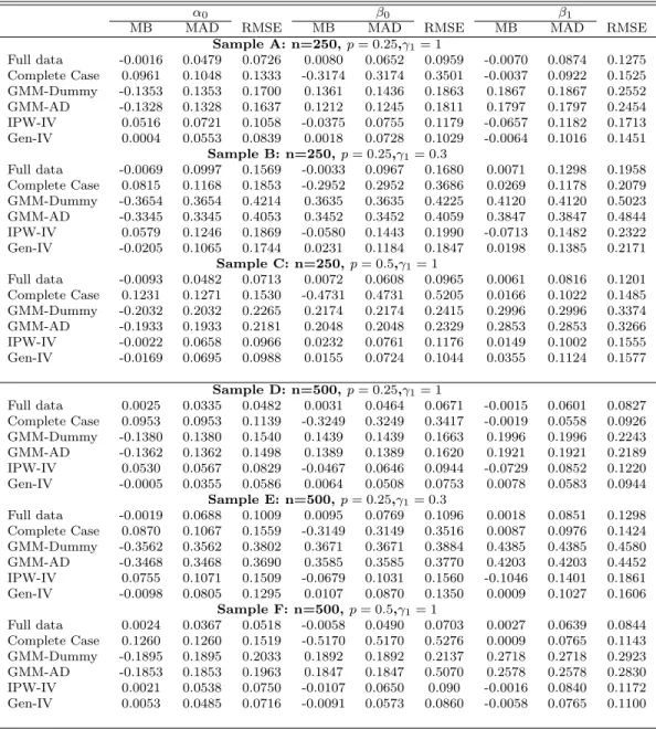
er-ror (RMSE). Table 1.1 and Table 1.2 contain the summary statistics for the estimators for each of the experiments. The case I consider most relevant for applications is in Table 1.1.

There is clear evidence that estimates of three estimators, the Complete Case estimator, GMM-Dummy estimator, and GMM-AD estimator are very biased. Both MB and MAD are much larger for these three estimators than those of the rest. The estimates are even more biased when the instrument is relatively weak, i.e. γ1 = 0.3. One possible reason for the biasedness is that all

the three estimators are based on the moment conditionE((1−Di)Zii) = 0.

When the missing indicatorDidepends onWi , it is plausible that the moment

condition E((1−Di)Zii) 6= 0. To see this more explicitly, note that under

Assumption 1and using Law of iterated expectations,

E((1−Di)Zii) =E(E((1−Di)Zii|Wi, Zi))

=E(E((1−Di)|Wi)Zii)

=E((1−p(Wi))Zii)

The full data moment function Zii is multiplied by the propensity

score 1−p(Wi), which could results in the inconsistency of estimation based

on this moment equation. This also explains the necessity for the IPW-IV and Gen-IV estimators to adjust the observed data moment function (1−Di)Zii

by the inverse of propensity score ₁₋_p1₍_W

i).

Since the error term i can be consistently estimated via Gen-IV, one

(43)

following null and alternative hypothesis:

H0 :E((1−Di)Zii) = 0

H1 :E((1−Di)Zii)6= 0

Overall, the Gen-IV estimator dominates the IPW-IV estimator in the perspective of every summary statistic. The performance of the Gen-IV esti-mator is the closest to that of the infeasible Full data estiesti-mator among all the estimators. Even when there is nearly one quarter of missing instruments, the summary statistics for the full data estimator and the Gen-IV estimator are still quantitatively similar.

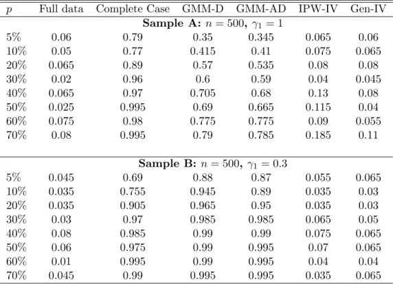
To further explore how the missing proportion will influence the behav-ior of estimators, I conduct a Wald-type test with “H0 : α0 = β0 = β1 = 1”

for a wide range of values of p, p ∈ {0.05,0.1,0.2,0.3,0.4,0.5,0.6,0.7}. I re-port rejection frequencies of 5% level tests for each of the six estimators under DGP1 in Table 1.3. The rejection frequencies for the three biased estima-tors, Complete Case, GMM-Dummy and GMM-AD are quite high, even if the missing proportionpis as low as 5%. When the instrument is relatively weak,

γ1 = 0.3, there are more than half of the iterations in which Complete Case,

GMM-Dummy, and GMM-AD estimators reject the null. However, there is no clear conclusion about the patterns of Gen-IV estimator and IPW-IV estima-tor. Both of them have similar rejection frequencies. And these frequencies are quantitatively similar compared to the Full data estimator. One interesting finding in Table 1.3is that the rejection frequencies for Gen-IV estimator and

(44)

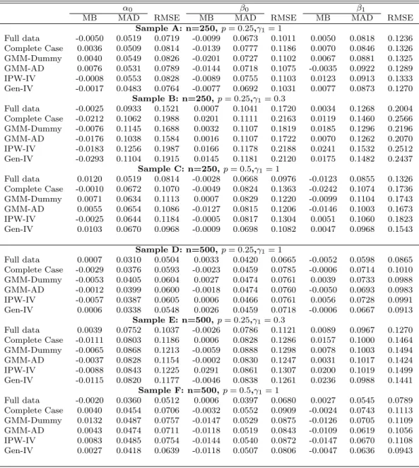
IPW-IV estimator won’t change much as the missing proportion increases. Table 1.2 summarizes the behavior of the six estimators under DGP2. SinceDi is completely exogenous, it holds that

E((1−Di)Zii) =E(1−Di)E(Zii)

| {z }

0

= 0

In this case, all the estimators are consistent. There does not seem to exist a best estimator in terms of MB and MAD. The Gen-IV estimator has slightly smaller RMSE than the others. In particular, the advantage of the Gen-IV estimator is more obvious when the missing proportion is higher, p = 0.5, or when the instrument is stronger, γ1 = 1.

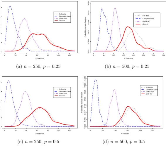
To compare the identifying power of instrument sets from different es-timators, I draw distributions of the F statistic from reduced form regression in Figure 1. These figures present density estimates of the F statistic when instrument Zi is relatively weak γ1 = 0.3 under DGP1. Results show that

the identifying power of generated instruments is very close to the full data instruments. On the other hand, restricting estimation within the complete data sample will severely contaminate the identifying power of IV. Sometimes when missing proportion is high (e.g., (c) n= 250, p= 0.5), researchers might get wrong conclusion about the strength of the instrument, with suspicion of weak instrument.

(45)

Figure 1.1: Distribution of the first-stage F statistic: DGP1 0 20 40 60 80 100 120 0.00 0.01 0.02 0.03 0.04 0.05 F Statistics

Probability density function

Full data Complete case GMM−AD Gen−IV (a) n= 250, p= 0.25 0 50 100 150 200 250 300 350 0.000 0.005 0.010 0.015 0.020 0.025 F Statistics

Full data Complete case GMM−AD Gen−IV (b)n= 500, p= 0.25 0 20 40 60 80 100 120 0.00 0.01 0.02 0.03 0.04 0.05 F Statistics

Full data Complete case GMM−AD Gen−IV (c)n= 250,p= 0.5 0 50 100 150 200 250 0.000 0.005 0.010 0.015 0.020 0.025 0.030 0.035 F Statistics

Full data Complete case GMM−AD Gen−IV

(46)

Table 1.1: Summary Statistics for DGP1

α0 β0 β1

MB MAD RMSE MB MAD RMSE MB MAD RMSE Sample A: n=250,p= 0.25,γ1= 1 Full data -0.0016 0.0479 0.0726 0.0080 0.0652 0.0959 -0.0070 0.0874 0.1275 Complete Case 0.0961 0.1048 0.1333 -0.3174 0.3174 0.3501 -0.0037 0.0922 0.1525 GMM-Dummy -0.1353 0.1353 0.1700 0.1361 0.1436 0.1863 0.1867 0.1867 0.2552 GMM-AD -0.1328 0.1328 0.1637 0.1212 0.1245 0.1811 0.1797 0.1797 0.2454 IPW-IV 0.0516 0.0721 0.1058 -0.0375 0.0755 0.1179 -0.0657 0.1182 0.1713 Gen-IV 0.0004 0.0553 0.0839 0.0018 0.0728 0.1029 -0.0064 0.1016 0.1451 Sample B: n=250,p= 0.25,γ1= 0.3 Full data -0.0069 0.0997 0.1569 -0.0033 0.0967 0.1680 0.0071 0.1298 0.1958 Complete Case 0.0815 0.1168 0.1853 -0.2952 0.2952 0.3686 0.0269 0.1178 0.2079 GMM-Dummy -0.3654 0.3654 0.4214 0.3635 0.3635 0.4225 0.4120 0.4120 0.5023 GMM-AD -0.3345 0.3345 0.4053 0.3452 0.3452 0.4059 0.3847 0.3847 0.4844 IPW-IV 0.0579 0.1246 0.1869 -0.0580 0.1443 0.1990 -0.0713 0.1482 0.2322 Gen-IV -0.0205 0.1065 0.1744 0.0231 0.1184 0.1847 0.0198 0.1385 0.2171 Sample C: n=250,p= 0.5,γ1= 1 Full data -0.0093 0.0482 0.0713 0.0072 0.0608 0.0965 0.0061 0.0816 0.1201 Complete Case 0.1231 0.1271 0.1530 -0.4731 0.4731 0.5205 0.0166 0.1022 0.1485 GMM-Dummy -0.2032 0.2032 0.2265 0.2174 0.2174 0.2415 0.2996 0.2996 0.3374 GMM-AD -0.1933 0.1933 0.2181 0.2048 0.2048 0.2329 0.2853 0.2853 0.3266 IPW-IV -0.0022 0.0658 0.0966 0.0232 0.0761 0.1176 0.0149 0.1002 0.1555 Gen-IV -0.0169 0.0695 0.0988 0.0155 0.0724 0.1044 0.0355 0.1124 0.1577 Sample D: n=500,p= 0.25,γ1= 1 Full data 0.0025 0.0335 0.0482 0.0031 0.0464 0.0671 -0.0015 0.0601 0.0827 Complete Case 0.0953 0.0953 0.1139 -0.3249 0.3249 0.3417 -0.0019 0.0558 0.0926 GMM-Dummy -0.1380 0.1380 0.1540 0.1439 0.1439 0.1663 0.1996 0.1996 0.2243 GMM-AD -0.1362 0.1362 0.1498 0.1389 0.1389 0.1620 0.1921 0.1921 0.2189 IPW-IV 0.0530 0.0567 0.0829 -0.0467 0.0646 0.0944 -0.0729 0.0852 0.1220 Gen-IV -0.0005 0.0355 0.0586 0.0064 0.0508 0.0753 0.0078 0.0583 0.0944 Sample E: n=500,p= 0.25,γ1= 0.3 Full data -0.0019 0.0688 0.1009 0.0095 0.0769 0.1096 0.0018 0.0851 0.1298 Complete Case 0.0870 0.1067 0.1559 -0.3149 0.3149 0.3516 0.0087 0.0976 0.1424 GMM-Dummy -0.3562 0.3562 0.3802 0.3671 0.3671 0.3884 0.4385 0.4385 0.4580 GMM-AD -0.3468 0.3468 0.3690 0.3585 0.3585 0.3770 0.4203 0.4203 0.4452 IPW-IV 0.0755 0.1071 0.1509 -0.0679 0.1031 0.1560 -0.1046 0.1401 0.1861 Gen-IV -0.0098 0.0805 0.1295 0.0107 0.0870 0.1350 0.0009 0.1027 0.1606 Sample F: n=500,p= 0.5,γ1= 1 Full data 0.0024 0.0367 0.0518 -0.0058 0.0490 0.0703 0.0027 0.0639 0.0844 Complete Case 0.1260 0.1260 0.1519 -0.5170 0.5170 0.5276 0.0009 0.0765 0.1143 GMM-Dummy -0.1895 0.1895 0.2033 0.1892 0.1892 0.2137 0.2718 0.2718 0.2923 GMM-AD -0.1853 0.1853 0.1963 0.1847 0.1847 0.5070 0.2578 0.2578 0.2830 IPW-IV 0.0021 0.0538 0.0750 -0.0107 0.0650 0.090 -0.0016 0.0840 0.1172 Gen-IV 0.0053 0.0485 0.0716 -0.0091 0.0573 0.0860 -0.0058 0.0765 0.1100

(47)

Table 1.2: Summary Statistics for DGP2

α0 β0 β1

MB MAD RMSE MB MAD RMSE MB MAD RMSE Sample A: n=250,p= 0.25,γ1= 1 Full data -0.0050 0.0519 0.0719 -0.0099 0.0673 0.1011 0.0050 0.0818 0.1236 Complete Case 0.0036 0.0509 0.0814 -0.0139 0.0777 0.1186 0.0070 0.0846 0.1326 GMM-Dummy 0.0040 0.0549 0.0826 -0.0201 0.0727 0.1102 0.0067 0.0881 0.1325 GMM-AD 0.0076 0.0531 0.0789 -0.0144 0.0718 0.1075 -0.0035 0.0922 0.1289 IPW-IV -0.0008 0.0553 0.0828 -0.0089 0.0755 0.1103 0.0123 0.0913 0.1333 Gen-IV -0.0017 0.0483 0.0764 -0.0077 0.0692 0.1031 0.0077 0.0873 0.1270 Sample B: n=250,p= 0.25,γ1= 0.3 Full data -0.0025 0.0933 0.1521 0.0007 0.1041 0.1720 0.0034 0.1268 0.2004 Complete Case -0.0212 0.1062 0.1988 0.0201 0.1111 0.2163 0.0119 0.1460 0.2566 GMM-Dummy -0.0076 0.1145 0.1688 0.0032 0.1107 0.1819 0.0185 0.1296 0.2196 GMM-AD -0.0176 0.1038 0.1584 0.0016 0.1107 0.1722 0.0070 0.1262 0.2070 IPW-IV -0.0183 0.1256 0.1987 0.0166 0.1178 0.2188 0.0241 0.1532 0.2512 Gen-IV -0.0293 0.1104 0.1915 0.0145 0.1181 0.2120 0.0175 0.1482 0.2437 Sample C: n=250,p= 0.5,γ1= 1 Full data 0.0120 0.0519 0.0814 -0.0028 0.0668 0.0976 -0.0123 0.0855 0.1326 Complete Case -0.0010 0.0672 0.1070 -0.0049 0.0824 0.1363 -0.0242 0.1074 0.1736 GMM-Dummy 0.0071 0.0634 0.1113 0.0007 0.0829 0.1220 -0.0099 0.1104 0.1743 GMM-AD 0.0055 0.0654 0.1086 -0.0127 0.0815 0.1206 -0.0146 0.1003 0.1673 IPW-IV -0.0025 0.0644 0.1184 -0.0005 0.0817 0.1304 0.0051 0.1060 0.1823 Gen-IV 0.0103 0.0670 0.0968 -0.0009 0.0698 0.1082 0.0047 0.0968 0.1543 Sample D: n=500,p= 0.25,γ1= 1 Full data 0.0007 0.0310 0.0504 0.0033 0.0420 0.0665 -0.0052 0.0598 0.0865 Complete Case -0.0029 0.0376 0.0593 -0.0023 0.0459 0.0785 -0.0006 0.0714 0.1010 GMM-Dummy -0.0053 0.0405 0.0604 0.0027 0.0474 0.0761 0.0039 0.0733 0.0988 GMM-AD -0.0012 0.0399 0.0600 -0.0018 0.0474 0.0760 -0.0050 0.0693 0.0983 IPW-IV -0.0057 0.0387 0.0605 0.0006 0.0466 0.0761 0.0056 0.0728 0.0991 Gen-IV 0.0006 0.0338 0.0548 0.0026 0.0459 0.0718 -0.0006 0.0667 0.0913 Sample E: n=500,p= 0.25,γ1= 0.3 Full data 0.0039 0.0752 0.1037 -0.0026 0.0786 0.1121 0.0089 0.0967 0.1270 Complete Case -0.0111 0.0803 0.1186 0.0006 0.0828 0.1286 0.0157 0.1000 0.1464 GMM-Dummy -0.0065 0.0868 0.1213 -0.0059 0.0888 0.1298 0.0078 0.1003 0.1494 GMM-AD -0.0037 0.0828 0.1154 -0.0002 0.0830 0.1247 0.0031 0.1017 0.1424 IPW-IV -0.0088 0.0843 0.1225 0.0291 0.0861 0.1307 0.0200 0.1019 0.1499 Gen-IV -0.0115 0.0820 0.1177 -0.0046 0.0838 0.1261 0.0236 0.0988 0.1441 Sample F: n=500,p= 0.5,γ1= 1 Full data -0.0020 0.0360 0.0512 0.0006 0.0397 0.0680 0.0027 0.0545 0.0789 Complete Case 0.0040 0.0454 0.0706 -0.0032 0.0552 0.0909 -0.0024 0.0743 0.1113 GMM-Dummy 0.0132 0.0487 0.0757 -0.0147 0.0529 0.0875 -0.0126 0.0705 0.1109 GMM-AD 0.0043 0.0474 0.0711 -0.0118 0.0519 0.0843 -0.0109 0.0619 0.1056 IPW-IV 0.0083 0.0485 0.0754 -0.0144 0.0540 0.0872 -0.0147 0.0670 0.1108 Gen-IV 0.0027 0.0418 0.0639 -0.0118 0.0507 0.0806 -0.0047 0.0636 0.0943

(48)

Table 1.3: Rejection Rates: DGP2

p Full data Complete Case GMM-D GMM-AD IPW-IV Gen-IV

Sample A: n= 500, γ1 = 1 5% 0.06 0.79 0.35 0.345 0.065 0.06 10% 0.05 0.77 0.415 0.41 0.075 0.065 20% 0.065 0.89 0.57 0.535 0.08 0.08 30% 0.02 0.96 0.6 0.59 0.04 0.045 40% 0.065 0.97 0.705 0.68 0.13 0.08 50% 0.025 0.995 0.69 0.665 0.115 0.04 60% 0.075 0.98 0.775 0.775 0.09 0.055 70% 0.08 0.995 0.79 0.785 0.185 0.11 Sample B: n= 500, γ1 = 0.3 5% 0.045 0.69 0.88 0.87 0.055 0.065 10% 0.035 0.755 0.945 0.89 0.035 0.03 20% 0.035 0.905 0.965 0.95 0.035 0.03 30% 0.03 0.97 0.985 0.985 0.065 0.05 40% 0.08 0.985 0.99 0.99 0.075 0.065 50% 0.06 0.975 0.99 0.995 0.07 0.065 60% 0.01 0.995 0.99 0.995 0.04 0.04 70% 0.045 0.99 0.995 0.995 0.035 0.065

(49)

1.6 Application

In this section, I apply the new estimation methodology to study the causal effect of education in labor market outcomes. It is well understood in the literature that education is endogenous. One of the famous candidate in-struments for education is the college proximity. Card(1995) uses an indicator for the presence of an accredited 4-year college in the local labor market as an instrument for education.

Other factors like ability affect both education and wage at the same time. Ability then enters into the wage regression as an important confounder. And there has been a long tradition in the literature to use “Knowledge of the World of Work” (KWW) test score13_{as a measure of “ability”, which can date} back toGriliches (1976),Griliches (1977). A potential criticism about KWW is that it is treated as an error-free measure of “‘ability”. To address this criticism, IQ score is used to instrument for the KWW score.

I use the following specification in this section:

lwagei =β0+β1 Educationi | {z } IV:college proximity +α KW Wi | {z } IV:IQ score +other controls0γ+i

where education and KWW score are instrumented by college proximity and IQ score, respectively. The dependent variable is the log of weekly wage.

13_{In the NLSYM76 dataset, the KWW test items were questions on the job activities of 10}

specific occupations, the education requirements for these 10 occupations, and the relative earnings of 8 different pairs of occupations, with a total of 28 items.

(50)

1.6.1 Data and Missing Instruments

The data sample consists of 2,963 observations on male workers from the National Longitudinal Survey of Young Men (NLSYM) in 1976. Other control variables include years of experience (and its square), an SMSA indi-cator (=1 if living in an SMSA in 1976), a South indiindi-cator (=1 if living in the south in 1976), and a black-race indicator. Regions dummies include 9 region indicators and family background consists of 14 variables representing mother’s and father’s education, indicators for missing father’s or mother’s education, interactions of mother’s and father’s education, and dummies for family structure at age 14.

The IQ data are missing for 923 observations. Thecomplete data sam-ple, where IQ scores are observed, has 2,040 observations.

Simulation studies in the previous section suggest that Complete Data method only works when the instrument is MCAR. Table 1.4 checks the de-pendence of the missing indicator on completely observed variables by running Logit and Probit regression ofDi onWi. Significant coefficients are found for

KWW, education, experience (and its square) and the South indicator. And results are robust if we include family background as well as the region dum-mies. There is clear evidence that IQ is not MCAR, which implies that the results under Complete Data method might not be reliable.

(51)

Table 1.4: Checking for MCAR of IQ

Missingness of IQ Score, (D)

Logit-I Probit-I Logit-II Probit-II Logit-III Probit-III

(1) (2) (3) (4) (5) (6) Wage -0.1685 -0.0927 -0.1633 -0.0890 -0.1618 -0.0886 (0.1221) (0.0708) (0.1227) (0.0711) (0.1243) (0.0718) Ability(KWW) -0.0307*** -0.0181*** -0.0285*** -0.0167*** -0.0275*** -0.0160*** (0.0072) (0.0042) (0.0073) (0.0043) (0.0074) (0.0043) Education -0.2529*** -0.1385*** -0.2285*** -0.1253*** -0.2338*** -0.1286*** (0.0223) (0.0125) (0.0235) (0.0132) (0.0237) (0.0133) Experience -3.1546*** -1.8111*** -3.2040*** -1.8415*** -3.2598*** -1.8744*** (0.3019) (0.1739) (0.3033) (0.1745) (0.3050) (0.1754) Experience squared 5.3667*** 3.0849*** 5.4426*** 3.1322*** 5.5355*** 3.1863*** (0.5236) (0.3016) (0.5258) (0.3025) (0.5286) (0.3040) Black 0.8172*** 0.5018*** 0.7046*** 0.4317*** 0.7160*** 0.4411*** (0.1188) (0.0708) (0.1239) (0.0737) (0.1251) (0.0744) SMSA -0.0258 -0.0110 -0.0138 -0.0058 -0.0008 0.0015 (0.1037) (0.0605) (0.1045) (0.0609) (0.1077) (0.0626) South 0.4307*** 0.2461*** 0.3959*** 0.2287*** 0.2604 0.1450 (0.1020) (0.0597) (0.1032) (0.0602) (0.2082) (0.1207) Constant 49.8121*** 28.4567*** 51.1235*** 29.2531*** 52.1515*** 29.8705*** (4.3385) (2.4941) (4.3757) (2.5105) (4.4036) (2.5246) Family background N N Y Y Y Y Region dummies N N N N Y Y N 2,963 2,963 2,963 2,963 2,963 2,963 1.6.2 Results

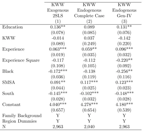
Table1.5reports the IV estimation results. Column (1) treats KWW as exogenous, as one of the specifications considered inCard(1995). It is served as a benchmark for the other two IV results. Column (2) is the procedure adopted in Card (1995) where IV estimation is conducted only to the complete data sample. Column (3) is based on the generated IQ scores. Results show that the return to education is insignificant using Complete Data method. Instead, the proposed method in this paper will restore the significance of return to education. Meanwhile, the standard errors of most of the coefficients are smaller compared to Column (2).

(52)

Table 1.5: Instrumental Variables Estimation of Return to Education

Weekly log(Wage)(Dependent variable)

KWW KWW KWW

Exogenous Endogenous Endogenous 2SLS Complete Case Gen-IV

(1) (2) (3) Education 0.136** 0.089 0.131** (0.078) (0.085) (0.076) KWW -0.014 0.037 -0.142 (0.089) (0.249) (0.220) Experience 0.063*** 0.059** 0.096*** (0.019) (0.035) (0.032) Experience Square -0.117 -0.112 -0.220** (0.108) (0.105) (0.092) Black -0.172*** -0.138 -0.256** (0.036) (0.119) (0.116) SMSA 0.091** 0.117*** 0.123*** (0.044) (0.025) (0.023) South -0.145*** -0.102*** -0.148*** (0.028) (0.032) (0.028) Constant 4.040*** 4.278*** 4.180*** (0.657) (0.654) (0.539) Family Background Y Y Y Region Dummies Y Y Y N 2,963 2,040 2,963

1.7 Conclusion

I study consistent and efficient IV estimation when instruments are missing endogenously. Under a conditional version of “missing at random” assumption, I am able to generate new instruments for every observation in the original data sample. With a generated instrument set, the identifying power of the infeasible full data instrument can be largely restored, making valid inference possible.

(53)

Empirical researchers need to be more cautious when facing missing instruments in the data set. If endogenous missingness exists, simply ignoring the observations with missing instruments may result in insignificant coeffi-cients of interest and very large standard errors. Furthermore, the diagnosis about the strength of IV could also be wrong.

There are several directions for future research. First, it is interest-ing to investigate other missinterest-ing data problems in IV estimation. Examples include missing endogenous variables and missing dependent variables. In-ference methods under other more complicated situations e.g. IV estimation entailing missing instruments and weak instruments would also worth a try. Second, one can develop formal tests on the consistency of Complete Data methods based on certain moment conditions. Also, the theoretical results in this paper has focused on monotone missing patterns of instruments. The idea of generated instruments can be extended to multiple/non-monotone missing-ness of instruments.

(54)

Chapter 2 Methods for Optimal Instruments with Many

Missing Instruments

2.1 Introduction

In this chapter, I study another case of missing instruments, i.e. many missing instruments. It occurs in empirical studies when one has a rich in-strument set but each inin-strument can have missing values. The methodology developed in this chapter is an extension to the generated instrument approach in Chapter 1. I also propose a three-step estimation procedure. In the first step, many generated instruments are formed and estimated. These generated instruments are used to improve the efficiency of IV estimation or approximate the infeasible optimal instruments in the spirit of Amemiya(1974), Chamber-lain (1987), andNewey (1990). Although the improvement in efficiency is at-tractive, there are two potential problems with generating many instruments. The first problem is the well-known “many-instrument” problem where the IV estimators based on many instruments may have poor properties.1 The second problem is the possible large estimation error in the formation of the many generated instruments. Keeping these two problems in mind, in the

1_{These poor properties include inaccurate inference and large standard errors. See}_Bekker

(55)

second step, I develop a shrinkage-based method for estimating the reduced form regression of the endogenous variable on the many generated instruments. My method can accomplish selection among many generated instruments and parameter estimates within one step. At the same time, it controls for the estimation bias brought by first-step estimation. I extend the methods of Bel-loni et al. (2012) to a pseudo-approximation of the optimal instruments. The IV estimation proceeds in the third step by regressing the dependent variable on the pseudo-approximation.

The approach is new and easy for implementation. It recovers the full data instrument set from the original many missing instruments. The new instrument set does not suffer from missing data issues again. I also allow a flexible instrument set in which the number of instruments can be increas-ing with the sample size and can even exceed the sample size. At the same time, every instrument in the instrument set could have missing values. Both

Muris (2011) and Chaudhuri and Guilkey (2013) consider multiple missing data problems including missing instruments. But the instrument set is fixed in their settings. To my knowledge, this is the first paper in the literature to study many missing instruments. In particular, I am able to show that under a “pseudo” sparsity condition and several regularity conditions, the parameters of interest are estimated at the parametric rate.

This paper also makes several theoretical contributions. First, I cal-culate semiparametric efficiency bounds under conditional moment equality when the conditioning variable has missing data. Hristache and Patilea(2014)