2009/51
■
Multi-assets real options
CORE
Voie du Roman Pays 34
B-1348 Louvain-la-Neuve, Belgium. Tel (32 10) 47 43 04
Fax (32 10) 47 43 01
E-mail: [email protected] http://www.uclouvain.be/en-44508.html
CORE DISCUSSION PAPER 2009/51
Multi-assets real options
Joachim GAHUNGU1 and Yves SMEERS2
September 2009
Abstract
Real options present a wide topic in investment litterature nowadays. However, despite big advances in the single asset investment pricing, the theory is miser of informations about problems involving more than one asset. We show in this paper that using dynamic programming, one can find an analytic trigger for a three assets simple exchange problem. Although we get a forward investment rule, one can not find the precise option value ex ante but only an average value. The precise option value depends on the first exit time from the continuation region which is stochastic.
This is a quite intuitive effect of the course of dimensionality of the problem. Valuating a single asset project gives a single condition for the optimal decision rule. The same holds for the simple exchange problem with two assets since the value of the project just depends on the price over cost ratio. In a three assets problem, as the project don’t depend anymore of a single state variable, one can’t run for a decision rule depending on the first exit time from the continuation region.
Keywords: real options, dynamic programming, price and cost uncertainty.
JEL Classification: C61, C63, G11
1 Université catholique de Louvain, CORE, B-1348 Louvain-la-Neuve, Belgium.
E-mail: [email protected]
2 Université catholique de Louvain, CORE and INMA, B-1348 Louvain-la-Neuve, Belgium.
E-mail: [email protected]. This author is also member of ECORE, the association between CORE and ECARES.
Financial support from GDF-Suez is gratefully acknowledged.
This paper presents research results of the Belgian Program on Interuniversity Poles of Attraction initiated by the Belgian State, Prime Minister's Office, Science Policy Programming. The scientific responsibility is assumed by the authors.
1
Introduction
A firm that observes a rise in demand of its output is induced to increase production to catch a higher immediate profit. To do so, it may have to invest in additionnal capacity. Sometimes, these investments have no salvage value. They are firm specific and hence cannot be recovered should the demand fall or the production cost rise. For instance, in power generation, a Combined Cycle Gas Turbine looses some of its value if the price of gas rises sharply and the utilisation of the plant decreases. There is little incentive for a competitor to buy the plant and hence no way to recover the entire initial expenditure. Such firm specific investment has a sunk cost : it is irreversible i.e. it cannot be recovered assuming downturn.
Irreversibility requires to act carefully. On one side, investing too early exposes to damages assuming downturn. On the other side, waiting implies lost immediate profits. One needs an investment rule that gives the perfect trade-off between the option to wait for a safer opportunity and the decision to go ahead with the investment as soon as one can capture an immediate profit.
The combination of the two features — irreversibility and time flexibility — im-plies an opportunity cost. Because of irreversibility, the opportunity to wait has a value that one must take into account in the investment decision. Investing entails not only the sunk cost of the project but also the cost of abandoning the option to invest later. The optimal behavior requires to wait until the value of launching the project just equals its sunk cost plus the opportunity cost of abandoning the right to wait. This is the well known analogy between investment problems and financial options : the right to delay an expenditure until an optimal time is similar to an american call
option. The option to wait can accordingly be priced using eithercontingent claimor
dynamic programmingdepending on whether the value of the project is or is not
per-fectly correlated with an asset traded on the market.1
Contingent claim analysis is the traditional approach for valuing options in fi-nance. It requires that the value of the project — here the option — is at all moment replicated by a portfolio of traded assets. The value ot the option at any time is then the market value of that portfolio. This approach is quite demanding in term of as-sumptions. The interested reader can consult Wilmott[18], Shreve[16], Karatzas and Shreve[7] and Bingham and Kiesel[3]. Theses assumptions do not always fit the real-ity of investment in some physical assets. For instance, one cannot replicate the value of a nuclear plant by a portfolio of traded assets, let alone do this on a continuous basis by continuously trading the elements of that portfolio. We therefore resort to the alternative approach of dynamic programming in the rest of the paper.
Dynamic programming avoids problems of market completeness or perfect cor-relation with some traded asset. There is no strong financial assumption except the existence of an exogeneous discount rate. This approach is more akin to classical cor-porate finance. It does not require spanning assets but supposes a discount rate that embeds risk aversion, referred to as a “risk discount rate”. The valuation of the option to wait by dynamic programming is based on Hamilton-Jacobi-Bellman equation. The essence of this method is to compare the immediate payoff coming from an immedi-ate investment to the expected payoff coming from the same delayed investment. One has to wait until the value of the immediate action exceeds the expected value of the delayed project.
Finding the optimal timing of an investment in a real asset implies identifying 1A comparison of these two approaches is given in Dixit and Pindyck[4].
the external conditions that justify the investment. More specifically one is looking for special values of the demand and/or of the cost that will trigger an irreversible investment. The set of the values is the border between the continuation region in which the optimal decision is to wait and the exploitation region, in which we launch the project. Because this border is initially unknown, real option problems are free boundary problems and the determination of the unknown bound needs a double sets of conditions known as value matching and smooth pastings (see section 2).
The notion of real option was developed by Myers[12]. The idea (see Myers[12], Kester[8]) to link investment opportunities and American call options leads to the simple result than the option to wait is an advantage that allows one to invest more safely. McDonald and Siegel[11] show in their seminal paper that the incentive to wait rises with the uncertainty of the project leading to the famous paradigm stated in Dixit and Pindyck’s book[4] : “(. . . ) the simple NPV rule is not just wrong; it is often very wrong.” Pindyck[14] notes the importance of delaying actions : for irreversible investment, one get one’s money’s worth waiting for new informations and higher value of the immediate post investment profit.
The theory of real option was extended from individual project valuation to the analysis of investment behaviour in market economics. Specifically, Leahy[9] shows that the optimal strategy of a firm acting in a competitive industry follows a myopic behavior. Oligopolistic situations were discussed by Slade[17], Baldursson[1], Bal-dursson and Karatzas[6]. Grenadier[5] finally proves than the Leahy’s myopic argu-ments still holds in symmetric oligopolies for Cournot competition.
The real options litterature usually treats a single uncertainty factor. Directly re-lated to our paper, the first two assets analysis was conducted by McDonald and
Siegel[11] with the problem of “price and cost uncertainty”.2 Additionnal work on
two assets uncertainty in irreversible investments includes Pindyck[15] and Bertola[2]. This paper extends the work of McDonald and Siegel[11]. It provides analytic so-lutions for more than two assets real options problems. McDonald and Siegel show that the two asset problem can be cast in the single state variable case and hence has a simple solution. With more than 2 assets one cannot reduce the problem to a single state variable and hence obtain an investment threshold that is given by a single num-ber. The boundary is a surface and hence the option value is not fully known before the first exit time of the continuation region. It is this problem with more than 2 assets that we examine in this paper.
We structure the work as follows : the second section presents the price and cost uncertainty problem. We prove that the solution found by McDonald and Siegel[11] is the only form that can solve the equation along with the value matching and the smooth pasting conditions. The third section is the presentation of the solution of the 3 assets exchange problem. Section 4 shows simulations and gives useful comments. Section 5 extends the discussion to more than 3 assets. Section 6 gives solutions to additional problems. Section 7 concludes.
2
The (1,1) exchange problem
The first two asset real option model has been developed by McDonald and Siegel[11], hereafter referred to as "the price and cost uncertainty" or the (1,1) exchange prob-2McDonald and Siegel[11] treated the first (one uncertainty) real option model — known as the
Mc-Donald and Siegel example — and the first two uncertainties problem — the price and cost uncertainty problem — in the same paper.
lem.3 Consider the American perpetual right to exchange one asset for an other. Every problem that we will define herafter concerns American and perpetual security. See Margrabe[10] for a similar non perpetual European right.
Definition 1(The (1,1) exchange problem). Consider the perpetual American option to pay the stochastic cost K(t)against a project of stochastic valueS(t). When is the right time to exercise this option?
We make the standard assumption of geometric Brownian motion processes and write
dS(t) = µSS(t)dt+σSS(t)dzS(t, ωS) dK(t) = µKK(t)dt+σKK(t)dzK(t, ωK)
withE[dzSdzK] =ρSKdtwheredzSanddzKare respectively theSandKWiener
incre-ments. We note :
• Ω=ΩS×ΩKthe set of all the events for the 2 processes.
• ω∈Ωa special event for the set of the 2 processes{S(t), K(t)}i.e.
ω= (ωS, ωK).
The single termωincludes the randomness of the two processes.
• We defineFtto be theσ-algebra generated by the two variables{S(s), K(s)}0≤s≤t.
Note that{Ft}is increasing i.e. Fs ⊂ Ft fors ≤t. The random processesSand
KareFt-adapted.
We use dynamic programming throughout the paper and noterthe risk discount
rate. It is of course not the risk-free interest rate : we work on the the real measure and adapt consequently the discount rate to risk aversion.
We define the continuation region as the region in which the exchange of assetK
against assetSis not optimal. One can write the Bellman equation on the continuation
region. The value of the projectFis obviously a function of the two economic variables
SandK. F(S, K) =max S−K, 1 1+rdtE h F(S, K) +dF S, K i
In the continuation region
F(S, K) = 1 1+rdtE h F(S, K) +dF S, K i
leading to the Bellman partial differential equation
µSSFS+µKKFK+ 1 2 σ2SS2FSS+σ2KK2FKK+2ρSKσSσKKSFSK −rF=0 (1)
that directly follows by the two dimensions Ito lemma.4 Note that the differential
equation (1) only holds on the continuation region. We refer to a solution of (1) as a Bellman function.
3We use dynamic programming instead of contingent claim in order to lay the ground of the
method-ology used in the following sections.
4For a formal derivation see Dixit and Pindyck[4], chapter 6, section 5, Price and cost uncertainty.
2.1 The homogeneity argument
McDonald and Siegel[11] state the solution of (1) as the following homogeneous func-tion.
F(S, K) =AKS K
β
(2)
IntroducingF(S, K) in the differential equation (1), one finds that βsatisfies the
fol-lowing quadratic equation
Q(β)≡ 1 2β(β−1) σ2S+σ2K−2ρSKσSσK +β(µS−µK) − (r−µK) =0 (3) hereafter referred to as the “fundamental quadratic” of the (1,1) exchange. This equa-tion is known (see e.g. Dixit and Pindyck[4]) to have both a positive and a negative root, the positive root being greater than one. Because the value of the project increases
withS, one must insert the positive root in the Bellman function.
Dixit and Pindyck[4] discuss various features of the solution of the characteristic equation. Specifically, the positive and negative roots respectively tend toward 1 and 0 as uncertainty increases.
In order to find the exchange trigger surface, one applies the two following optimal investment conditions.
1. The value matching condition : at the optimal exercise time τ, the value of the
investment option matches the value of lauching the project i.e.
F(S(τ), K(τ)) =S(τ) −K(τ).
2. The smooth pasting conditions : at the optimal exercise point, the value of the
project must be smooth with respect to the S and K variables. See Dixit and
Pindyck[4] in chapter 4, Appendix C for a formal proof.
[∂SF] (S(τ), K(τ)) = 1 [∂KF] (S(τ), K(τ)) = −1
The derivation of the final result follows McDonald and Siegel[11] and is now stan-dard.
Proposition 1(Optimal trigger of the (1,1) exchange problem). The trigger of the (1,1) exchange problem is given by
T1 ≡ (S, K) | S= β1 β1−1K (4) whereβ1is the positive root of the fundamental quadraticQ(β).
Proof. See McDonald and Siegel[11] or Appendix A.
We note this trigger T1 to indicate that this relation define a 1-dimensional
man-ifold in theS×Kspace. Note that this result is strikingly similar to the investment
trigger of the single uncertain factor problem. The only difference is thatKnow
rep-resents a random variable. One can find an expression for the volatility and the drift of the exchange and thus fall back on the single asset rule. Such simplification also appears in Margrabe[10].
The right time to exercise the option is the first exit time from the continuation
region. It is given by a random timeτ(ω)defined by
τ(ω) =min
t | S(t, ω) = β1
β1−1K(t, ω)
where the vertical bar|means “such that”. If the eventS(t, ω) = β1
β1−1K(t, ω)has zero
measure, we setτ(ω) = +∞.
The continuation region is given by
CR ≡
(S, K) | S≤ β1
β1−1K
and because the random timeτ:ω →[0,∞]is the first exit time from a given subset
CR ∈R2,τis a stopping time (see Oksendal[13]).
2.2 Elaboration of the solution : the uncorrelated case
It is worth elaborating on the form of equation (2), starting from the uncorrelated exchange problem and seeing what variable separation brings us. Consider the case where there is no correlation. The partial differential equation simplifies to
µSSFS+µKKFK+ 1 2
σ2SS2FSS+σK2K2FKK−rF=0. (5) Assume a multiplicative form for the solution.
F(S, K) =Af(S)g(K)
withA > 0. The problem becomes separable as one can rewrite this differential
equa-tion as an equality between a funcequa-tion of S and a function of K. One can find the
solution of this two dimensional real option problem by solving two separate one di-mensional real option problems. Mathematically, one can prove that the multiplicative solution has to be of the formASβ1Kλ2.
Proposition 2(The power form of the (1,1) exchange). Assuming a separable form for the Bellman function of the (1,1) exchange, it has the power form
F(S, K) =ASβ1Kλ2 (6)
whereβ1andλ2 are the roots of two fundamental quadratics.
Proof. See Appendix A.
Assuming this particular solution, one can then prove that this function has to be homogeneous of degree one to satisfy the value matching and the smooth pasting conditions.
Applying the smooth pasting conditions one obtains
Proposition 3(Condition at trigger). At an optimal exercise timeτ, the point(S(τ), K(τ))∈
T1verifies S(τ) = − β1 λ2 K(τ) (7)
Proof. Using the solution F(S, K) = ASβ1Kλ2 in the two smooth pasting conditions leads to the two relations
β1
S(τ)F(S(τ), K(τ)) = 1 (8)
λ2
K(τ)F(S(τ), K(τ)) = −1. (9)
The two processesS(t, ω) andK(t, ω)will always be positive because zero is an
ab-sorbant barrier for the geometric Brownian motion. MoreoverF(S, K) is the value of
an option, so it has to be greater or equal to zero. Thus these two equations implies thatβ1 > 0and thatλ2 < 0. Now, we note that(8) = −(9)i.e.
β1
S(τ)F(S(τ), K(τ)) = − λ2
K(τ)F(S(τ), K(τ))
and we simplify byF(S(τ), K(τ))leading to
S(τ) = − β1 λ2 K(τ) (10)
which proves the statement.
One observes that the combination of the two smooth pastings leads to one trigger
condition. Simplifying by the function F(S(τ), K(τ)) eliminates the unknown
coeffi-cientAso the set of the two smooth pastings (8) and (9) is equivalently reformulated
as the trigger (7) plus one of these two smooth pastings.
Solving for the value matching condition leads to homogeneity result.
Proposition 4(Homogeneity in the (1,1) exchange problem). The Bellman function (6) of the (1,1) exchange problem satisfies
β1+λ2 =1 (11)
withβ1> 1andλ2 < 0. Proof. See Appendix A.
This proposition shows that homogeneity should not be seen as an assumption. It is imposed by the value matching and the smooth pasting conditions in the exchange of two assets.
Knowing that the sum of the positive root β1 and the negative root λ2 must be
equal to one, one can rewrite the general solution with a single exponent.
F(S, K) =AK S
K β1
(12) This is just the McDonald and Siegel[11] form. To solve the Bellman differential
equa-tion,β1 has to be the positive root of the quadratic equation
Q(β)≡ 1 2β(β−1) σ2S+σ2K +β(µS−µK) − (r−µK) =0.
One can similarly fall back on McDonald and Siegel trigger of Proposition 1 by
This variable separation also shows that one can alternatively write
F(S, K) =AS K
S λ2
without any difference of results. In the first formulation, the exchange option is
ex-pressed as a dynamic portfolio containing K(t, ωK) perpetual american calls on
un-derlying asset S(t, ωS)/K(t, ωK) and of strike one. In the second, it is expressed as
a dynamic portfolio containingS(t, ωS)perpetual american puts on underlying asset
K(t, ωK)/S(t, ωS) and of strike one. The two options are obviously the same. This dual view of the problem is known as changing numéraire in risk neutral valuation. See e.g. Shreve[16], Wilmott[18] or Bingham and Kiesel[3] for exhaustive informations on changing numéraire.
This discussion gave a motivation for the multiplicative form of the McDonald and Siegel[11] solution : We first noted that in the absence of correlation, the Bellman differential equation is separable so the multiplicative form comes naturally in mind. We then noticed that solving our differential equation with the value matching and smooth pastings conditions requires homogeneity for the Bellman function. We now extend these findings to the general correlated case.
2.3 Elaboration of the solution : the correlated case
Putting back correlation in the differential equation, one cannot infer directly a separa-ble form for the Bellman function and hence Proposition 2 no longer holds. However one can still try its multiplicative form
F(S, K) =ASβ1Kλ2.
One observes that this function solves Bellman differential equation with correlation and has to be homogeneous to solve the value matching and the smooth pasting con-ditions. Propositions 3 and 4 obviously still hold, leading to
Proposition 5(The general solution of the (1,1) exchange problem). The Bellman func-tion of the (1,1) exchange problem is given by
F(S, K) =AKS K
β1
(13) withβ1the positive root of a fundamental quadraticQ(β) : R→R.
Proof. One can check by direct calculus that the solution (13) solves the Bellman partial differential equation with correlated assets along with the value matching and smooth
pasting conditions. This only requiresβ1 to be the positive root of the more involved
fundamental quadratic
Q(β)≡ 1
2β(β−1)
σ2S+σ2K−2ρSKσSσK+β(µS−µK) − (r−µK) =0
3
The (2,1) exchange problem
The previous problem is a particular case of a wider class of problems defined as the
(n, m)exchange problem.
Definition 2 ((n,m) exchange problem). Consider the perpetual american option to ex-change a bundle ofnstochastic assets against a bundle ofmothers. When is the right time to exercise this option?
McDonald and Siegel[11]’s "price and cost uncertainty" is thus a (1,1) exchange that we extend to a (2,1) exchange problem in this section. Of course, if one can solve the (2,1) exchange problem, one can also solve the (1,2) exchange problem in a similar way.
Example 1. [The (2,1) exchange problem] Consider the perpetual American option to pay the sum of two stochastic sunk costsK1(t)andK2(t)for a project of stochastic valueS(t). When is the right time to exercise this option?
The three assets follow geometric Brownian motions i.e. :
dS(t) = µSS(t)dt+σSS(t)dzS(t, ωS)
dK1(t) = µK1K1(t)dt+σK1K1(t)dzK1(t, ωK1) dK2(t) = µK2K2(t)dt+σK2K2(t)dzK2(t, ωK2)
We allow for correlation between random processes. AssumeE[dzSdzK1] = ρSK1dt,
E[dzSdzK2] =ρSK2dt,E[dzK1dzK2] =ρK1K2dt. We note :
• Ω=ΩS×ΩK1×ΩK2 the set of events for the 3 processes.
• ω∈Ωa special event for the set of the 3 processes{S(t), K1(t), K2(t)}i.e.
ω= (ωS, ωK1, ωK2).
The single termωincludes the randomness of the three processes.
• We defineFt to be theσ-algebra generated by the random variables
{S(s), K1(s), K2(s)}0≤s≤t. Note that{Ft}is increasing i.e. Fs ⊂ Ftfors ≤t. The
random processesS,K1 andK2 areFt-adapted.
The following discussion essentially adapts the procedure of the (1, 1) exchange
problem to derive the Bellman function. We first solve the separable problem and show that the value matching and the smooth pasting conditions imply a homoge-neous form for the Bellman function. We then analyse the specific behavior of this three assets exchange problems.
3.1 The free boundary problem
The investment trigger is the set of all the triplets(S, K1, K2)for which it is optimal to
invest. We shall show that it is a surface — or a 2-dimensional manifold — in the 3
dimensional spaceS×K1×K2. This 2-dimensional manifold splits the whole space in
The right time to exercise the option is the first exit time from the continuation region. In other terms, this is the first time when one hits the trigger surface. This is a
random timeτ:Ω→[0,∞]. We note
τ:ω→τ(ω).
In a two variables problem — the (1,1) exchange — one observed that the right time to invest was given by an equation linking the two variables of the problem :
the trigger condition has the formS∗ = αK∗. The set of optimal couples (S∗, K∗) is
therefore a line in theS×Kplan. The right time to exercise the option is
τ=min
t | S(t) =αK(t)
.
In a three variables problem — like the (2,1) exchange — it is thus natural to expect that the investment trigger is a surface. One should find a 2-dimensional set of triplets
(S∗, K∗1, K∗2) satisfying the optimal investment criterion. We expect something of the
form
τ=min
t | S(t), K1(t), K2(t) ∈T2
withT2designating a 2-dimensional manifold.
This investment trigger T2 is the unknown bound of a free boundary problem.
Specifically, one needs to find the Bellman functionF(S, K1, K2)and the bound surface
T2such that :
• The Bellman functionF(S, K1, K2)solves
µSSFS + µK1K1FK1+µK2K2FK2 + ρSK1σSσK1SK1FSK1 + ρSK2σSσK2SK2FSK2 + ρK1K2σK1σK2K1K2FK1K2 + 1 2 σ2SS2FSS+σ2K1K 2 1FK1K1+σ 2 K2K 2 2FK2K2 −rF=0 (14)
in the continuation region.
• At each point S(τ), K1(τ), K2(τ)
∈ T2, the value of the project matches the
investment cost plus the option to defer : 1. In value (value matching)
F S(τ), K1(τ), K2(τ)=S(τ) −K1(τ) −K2(τ).
2. In slope (smooth pastings)
[∂SF] S(τ), K1(τ), K2(τ) = 1 [∂K1F] S(τ), K1(τ), K2(τ) = −1 [∂K2F] S(τ), K1(τ), K2(τ) = −1.
3.2 The uncorrelated case
Like in the two assets problem, we motivate the form of the Bellman function starting from the no correlation case. With this assumption, the differential equation in the continuation region becomes
µSSFS + µK1K1FK1+µK2K2FK2 + 1 2 σ2SS2FSS+σ2K 1K 2 1FK1K1 +σ 2 K2K 2 2FK2K2 −rF=0.
We can assume the separable multiplicative form
F(S, K1, K2) =Af(S)g(K1)h(K2)
for the Bellman function, whereAis a constant to determine.
The functionF(S, K1, K2)represents the value of the option to exchange the sum of
K1(t)andK2(t)forS(t). It must be increasing inSand decreasing in bothK1 andK2.
The problem is separable as we first assume no correlation between random processes. Solving using variable separation leads to the following result.
Proposition 6(The power form of the (2,1) exchange). Assuming a separable form for the Bellman function of the (2,1) exchange, it has the power form
F(S, K1, K2) =ASβ1Kλ2
1 K γ2
2 (15)
whereβ1,λ2andγ2are the roots of three fundamental quadratics.
Proof. See Appendix B.
Assuming this particular solution, one will prove that this function has to be homo-geneous of degree one to solve the value matching and the smooth pasting conditions.
The application of the smooth pasting conditions leads to
Proposition 7(Conditions at trigger). At an optimal exercise timeτ, the point(S(τ), K1(τ), K2(τ))∈
T2verifies K2(τ) = γ2 λ2 K1(τ) (16) S(τ) = − β1 λ2 K1(τ) (17)
whereβ1,λ2andγ2are the exponents of the separable Bellman function (15). Proof. Introducing the solution F(S(τ), K1(τ), K2(τ)) = ASβ1(τ)Kλ2
1 (τ)K γ2
2 (τ) in the
three smooth pasting conditions leads to the three relations
β1 S(τ)F(S(τ), K1(τ), K2(τ)) = 1 (18) λ2 K1(τ)F(S(τ), K1(τ), K2(τ)) = −1 (19) γ2 K2(τ)F(S(τ), K1(τ), K2(τ)) = −1. (20)
BecauseF(S(τ), K1(τ), K2(τ))is positive,β1has to be positive andλ2andγ2has to be
negative.
Then we note that(18) = −(19)and(19) = −(20). Simplifying byF(S(τ), K1(τ), K2(τ))
The three smooth pastings lead to two trigger conditions. The simplification by
the functionF(S(τ), K1(τ), K2(τ))eliminates the unknown coefficientAthen the set of
the three smooth pastings (18), (19) and (20) is equivalent to the set of the conditions at trigger (16) and (17) plus one of these three smooth pastings.
From now on we focus on the two conditions at trigger (16) and (17).
K2(τ) K1(τ) = γ2 λ2 S(τ) K1(τ) = −β1 λ2
For a given triplet(β1, γ2, λ2), these two relations define a 1-dimensional manifold
that gives a relation linking the priceS(τ)and the costsK1(τ)andK2(τ)at each
exer-cice timeτ. To find the investment trigger, one has to find the set of allowed triplets
{(β1, λ2, γ2)}which we shall show is itself a 1-dimensional manifold. Then one obtains
the trigger surface as the cartesian product of these two 1-dimensional manifolds. We begin by noting that the right time to exercise the option is the first exit time from the continuation region given by
τ=min t | K2(t) K1(t) = γ2 λ2, S(t) K1(t) = − β1 γ2,(β1, λ2, γ2)∈Σ .
We now characterise the setΣ.
From Proposition 7 and using the value matching
F(S(τ), K1(τ), K2(τ)) =S(τ) −K1(τ) −K2(τ)
one can expressAin terms of valueS(τ).
1 A =β1S β1−1(τ)Kλ2 1 (τ)K γ2 2 (τ) =β1S β1−1(τ) −λ2 β1 λ2 Sλ2(τ) −γ2 β1 γ2 Sγ2(τ) (21) Applying the value matching condition with the relations (21), (16) and (17) leads to homogeneity result.
Proposition 8(Homogeneity in the (2,1) exchange problem). The Bellman function (15) of the (2,1) exchange problem satisfies
β1+λ2+γ2 =1 (22)
withβ1> 1andλ2, γ2< 0.
Proof. See Appendix B.
Rewriting the Bellman function as
F(S, K1, K2) =ASK1 S λ2K2 S γ2 (23)
and introducing the homogeneity condition in (21) one obtains the coefficientA in
terms ofλ2 andγ2.
A(λ2, γ2) = 1
(1−λ2−γ2)(1−λ2−γ2)(−λ
2)λ2(−γ2)γ2
Note that the homogeneity condition reduces the possible values for the triplets
(β1, γ2, λ2) : one has 3 unknowns values and one condition then the set of possible
triplets become a 2-dimensional manifold.
One can rewrite our stopping time solution as :
τ=min t | K2(t) K1(t) = γ2 λ2, S(t) K1(t) = λ2+γ2−1 λ2 ,(λ2, γ2)∈Σ 0
where the setΣ0 remains to define. Substituting the solution (23) in the uncorrelated
Bellman partial differential equation (14), one find that the couple (λ, γ) solves the
following equation. Q(γ, λ) ≡ 1 2λ(λ−1) σ2S+σ2K 1−2ρSK1σSσK1 +λ(µK1−µS) + 1 2γ(γ−1) σ2S+σ2K 2−2ρSK2σSσK2 +γ(µK2−µS) − (r−µS) =0.
The right time to exercise the option is thus given by
τ=min t | K2(t) K1(t) = γ2 λ2, S(t) K1(t) = λ2+γ2−1 λ2 ,Q(γ2, λ2) =0 .
3.3 The correlated case
The problem is no longer separable in the correlated case and Proposition 6 no longer holds. One can still try the multiplicative form
F(S, K1, K2) =Sβ1Kλ2
1 K γ2
2
to check whether it verifies the differential equation (14) with correlation.
One observes that this function solves the Bellman differential equation with corre-lation and has to be homogeneous to solve the value matching and the smooth pasting conditions. Propositions 7 and 8 still hold and can be restated as follows :
Proposition 9(The general solution of the (2,1) exchange problem). The Bellman func-tion of the (2,1) exchange problem is given by
F(S, K1, K2) =A(λ2, γ2)S K1 S λ2K2 S γ2 (25) where (λ2, γ2) belong to the 0-level curve of an interaction fundamental quadratic form
Q(λ, γ) :R2 →RandA(λ2, γ2)is defined by relation (24).
Proof. One can check by direct calculus that the solution (25) solves the Bellman differ-ential equation with correlated assets along with the value matching and the smooth pastings conditions.
Substituting the general solution (25) in the differential equation (14), one find that
the couple(λ, γ)has to solve the following equation.
Q(λ, γ) ≡ 1 2λ(λ−1) σ2S+σ2K 1−2ρSK1σSσK1 +λ(µK1−µS) + 1 2γ(γ−1) σ2S+σ2K 2−2ρSK2σSσK2 +γ(µK2−µS) + λγσ2S−ρSK1σSσK1 −ρSK2σSσK2 +ρK1K2σK1σK2 − (r−µS) =0. (26)
Extending the previous notation, we refer to the binary quadratic form Q(γ, λ)
as the fundamental quadratic form of the problem.5 We refer to the values(λ, γ) for
which this quadratic form vanishes as the 0-level curve6ofQ(γ, λ).
This 0-level curve now reduces the possible set of triplets (β1, λ2, γ2) to a
1-dimensional manifold. One can then write the final expression of the investment trigger.
Proposition 10. The right time to exercise the option is the first exit time defined by
τ=min t | K2(t) K1(t) = γ2 λ2 , S(t) K1(t) = λ2+γ2−1 λ2 ,Q(λ2, γ2) =0 .
Proof. The result was directly derived from the preceding propositions. We now summarise the steps leading to the solution.
• Using the smooth pastings conditions, one obtains a 1-dimensional manifold for
the investment trigger. This manifold is parametrised by the triplet(β1, γ2, λ2).
• Using the value matching condition and the differential equation, one obtains
two conditions on the triplets (β1, γ2, λ2) : an homogeneity condition and a
quadratic form. Both conditions reduce the allowed triplets(β1, γ2, λ2) to a
1-dimensional manifold.
• To find the trigger, one has to introduce the 1-dimensional manifold for
(β1, γ2, λ2) in the 1-dimensional manifold for the trigger : this defines the
2-dimensional manifold for the general trigger.
3.4 Remarks
Note four points on Proposition 10 :
1. The right time to exercise the option allows one to determine the trigger surface. T2 ≡ (S, K1, K2) | K2 K1 = γ2 λ2, S K1 = λ2+γ2−1 λ2 , Q(λ2, γ2) =0 (27) One can write two alternative descriptions of the trigger using the conditions (16) and (17). Direct calculus leads to the following two other sets.
T2 ≡ (S, K1, K2)| K2 K1 = γ2 λ2 , S K2 = λ2+γ2−1 γ2 , Q(λ2, γ2) =0 (28) T2≡ (S, K1, K2) | K2 K1 = γ2 λ2, S= λ2+γ2−1 λ2+γ2 (K1+K2), Q(λ2, γ2) =0 (29) The formulation (29) of the trigger is meaningful : it is a direct link between the
revenue and the total cost. Both λ2 and γ2 are negative, thus the real option factor
(λ2+γ2 −1)/(λ2+γ2)in (29) is always higher than 1. We’ll show in Section 4.1 that it is also strictly increasing with the volatility of the three assets.
5A quadratic form in 2 variables is called a binary quadratic form. 6One can also use the terminology of 0-contour line.
2. T2 is the cartesian product of the set of possible triplets(S, K1, K2) assuming
known values for the triplet (β1, γ2, λ2) by the set of possible triplets {(β1, γ2, λ2)}. Since this is the product of two 1-dimensional manifold, the resulting set is a two dimensional manifold, as expected.
We note S(τ), K1(τ), K2(τ), β1, γ2, λ2 | {z } D=2 = S(τ), K1(τ), K2(τ)(β1, γ2, λ2) | {z } D=1 ⊗ (β1, γ2, λ2) | {z } D=1
3. The (2,1) problem differs from the (1,1) problem by a major feature : one does not know the value of the two exponents in the Bellman solution before reaching the trigger. The Bellman function is indeed only known when reaching the trigger; it can take different values because the trigger surface is a manifold of dimension greater than 1.
4. Finally, the preceding expression forτis a stopping time. One can write :
ω | τ(ω)≤t = ω | ∃t0 ≤0 : K2(t0) K1(t0) = γ2 λ2, S(t0) K1(t0) = λ2+γ2−1 λ2 ,Q(λ2, γ2) =0 Usingγ2 =λ2KK2(t0)
1(t0) this can be rewritten
ω | τ(ω)≤t = ω | ∃t0 ≤0 : S(t0) K1(t0) = λ2+λ2KK2(t0) 1(t0)−1 λ2 ,Q λ2, λ2K2(t0) K1(t0) =0 ∈ Ft
since the process K2(t)
K1(t) isFt-mesurable. Thenτ(ω) is a stopping time.So one can
de-termine whether or not the trigger has been reached at timetbased on informations
available up to time t. This investment rule is therefore appropriate to forward
nu-merical simulation as discussed in the following section.
A convenient reformulation of the trigger obtains after introducing the new stochastic process
η(t) = K2(t) K1(t)
∀t, η(t)∈ Ft.
One can write
τ(ω) =min t | S(t) K1(t) = λ2+λ2η(t) −1 λ2 ,Q(λ2, λ2η(t)) =0
and the trigger is defined by the collection of 1-dimensional manifoldC1(η)
T2 ={C1(η)}η>0 = (S, K1, K2) | S K1 = λ2+λ2η−1 λ2 ,Q(λ2, ηλ2) =0 η>0 parametrised by η= K2 K1.
In order to pave the way for numerical solution, the following section restate the opti-mal exercise procedure in algorithmic form.
3.5 Optimal exercise algorithm
1. Based on observations at timet, compute the ratio of the costs, notedη(t).
K2(t) K1(t)
=η(t)
2. In the fundamental quadratic form, replace γby ηλand solve for λ. Set λ2 =
min{λ}.
3. Using the last computedλ2, computeγ2 = ηλ2 to find the trigger value for the
price by S∗(t) = λ2+γ2−1 λ2 K1(t). 4. IfS=S∗ thent=τand F(S, K1, K2) =A(λ2, γ2)SK1 S λ2K2 S γ2 .
IfS6=S∗ then wait until timet+dtand return to step 1.
A detailed explanation of the algorithm is given in Appendix B.
As indicated above the value of the Bellman function depends on the first exit time. As this cannot be predicted one cannot give the precise Bellman function before the first exit time. One can however define the expected value of the Bellman function where the expectation is taken over the possible exit times. This cannot be solved analytically but is amenable to simulation. This is what we turn to in the next section.
4
Simulations
We here illustrate the three assets exchange problem by a few simulations. We conduct our analysis in four steps.
We first give standard comparative statics. Starting from a basic set of parameters we illustrate the variation of the trigger with respect to the drift rates, the volatility rates and the correlations. We show that our solution has a good real option behavior. The trigger increases with high volatitily rates and high drift rates for the price. The trigger decreases with the two costs drifts rates since increasing costs imply that it is more valuable to invest now than wait and incur a bigger cost. As explained before,
the trigger is a function of theK2/K1 ratio. Proper comparative must be conducted
with a fixed cost ratio. We therefore assume a constantK2/K1ratio for all the
compar-ative statics simulations.
In a second step, we use Monte Carlo simulation to find the probability distribution of the costs ratio at the first exit time.
We thirdly use this distribution to compute an expected Bellman function of the exchange problem.
Finally, we check that the binary quadratic form behave well under reasonnable assumptions on the diffusion processes.
4.1 Comparative Statics
We illustrate the behavior of our solution. We start from the following set of parame-ters. The discount rate is 5% and all rates are annual.
µS = 0.03 µK1 =0.015 µK2 =0.008
σS = 0.2 σK1 =0.25 σK2 =0.2
We split the year in 100 periods of time and scale variances accordingly. Correlations areρSK1 =0.15,ρSK2 =0.25,ρK1K2 = 0.75. We consider the cost ratioK2/K1 =0.8for the base case simulation and throughout the comparative statics.
For the base case simulation, we find a trigger
S∗=3.4965K1
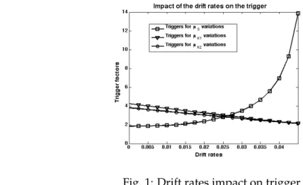
and find a real option factor greater than 1.8 as expected.7 Assume that we want to
see the impact of a change in theµS parameter. We plot the trigger starting from the
base case and changingµSover a broad range of values. We then do the same forµK1
andµK2 and obtain Figure 1, that depicts the impact of the drift rates on the trigger.
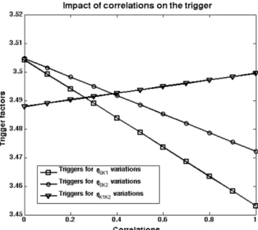
We do the same thing for the volatility rates and correlations to obtain Figure 2 and Figure 3.
Fig. 1: Drift rates impact on trigger
7This factor encompasses the two costs then must be twice bigger than normal. One can check that
putting all drift rates, all volatility rates and all correlations to zero lead to a trigger factor equal to 1.8 i.e. the deterministic rule since we assumedK2/K1=0.8.
Fig. 2: Volatility rates impact on trigger
Fig. 3: Correlations impact on trigger
Figure 1 shows that the trigger is an increasing function of the drift rate of the reselling price i.e. the incentive to wait is increasing with the expected profit’s growth. The value of the option to defer bursts when the drift rates rises up to the discount rate : it is then always more valuable to wait. However the trigger decreases with the cost’s drift rates as they reduce the expected spread.
Figure 2 shows that the trigger always increases with the volatility rates. Increasing uncertainty on the reselling price makes the option to wait for better safety more valu-able whereas an increasing uncertainty on a cost is an incentive to wait for a downturn in this cost.
Figure 3 shows that the trigger is a decreasing function of the correlation between the cost and the reselling price as this correlation reduces the expected spread. Con-versely, the real option trigger rises with the inter-cost correlation as it increases the uncertainty over the spread.
We conclude that the three assets model complies with standard intuition on real options. As the uncertainty increases the option to postpone investment has a greater value and thus leads to wait. The drift is also a key parameter as a higher expected growth leads to a bigger incentive to wait for better conditions. The correlation factors have different impacts depending on their link with the reselling price. A correlation between the reselling price and a cost decreases the uncertainty over the spread and
thus reduces the investment trigger. A correlation between costs increases the uncer-tainty over the spread and thus increases the investment trigger.
4.2 Probability of the first exit time
Section 3.5 summarises the investment rule. As explained earlier it depends on the
first exit time of the continuation region through the stochastic parameterη(τ)defined
as
η(t) = K2(t) K1(t)
, ∀t.
At a exercise timeτ, this parameter satisfies
K2(τ) K1(τ) =η(τ) = γ2 λ2 S(τ) = λ2+γ2−1 λ2 K1(τ)
where(γ2, λ2)satisfies the 0-level curve of the fundamental quadratic (26). Suppose
one would know the probability distribution of the random variable η(τ), that is
dP[η(τ) = η]. It’s direct computation can be algebraically tricky, but it can be esti-mated using direct Monte Carlo method by resorting on our forward investment rule.
Suppose this is done, we note this probability densityφ(η).8
dP h
η(τ) =η i
=φ(η)dη
One can compute easily an expected value for the project.
Proposition 11 (The expected Bellman function of the project). Consider the (2,1) ex-change problem. Given the probability densityφ(η)of the costs ratio at the first exit time one can compute an expected Bellman function of the projectF(S, K¯ 1, K2).
¯ F(S, K1, K2) = Z+∞ 0 φ(η)A(η)S K1 S λ2(η)K2 S ηλ2(η) dη (30)
withA(η) =A(λ2(η), ηλ2(η)).
The expected value of the project is a function ofS, K1 andK2. We notedλ2(η)
becauseλ2is the negative root of the fundamental interaction quadratic formQ(λ, ηλ)
then it is unique and depends only on the value of the parameterη. For the same
reason, the coefficientA(λ2, ηλ2)is just a function ofη.
As we said earlier one can evaluate the probability density of the costs ratio at the first exit time using Monte Carlo method. This is done by simulating the evolu-tion of the risk factors using the decision rule on a big number of scenarios to have a
distribution of theηparameter associated with (the) exercise time.
We here give the graph of φ(η), the costs ratio distribution estimated by 15000
investment outcomes forηcorresponding to (the) first exit time. This graph shows a
bell-like curve for the costs ratio distribution. One can then have an approximation of the value of the project.
8To be more explicit P » η−dη 2 ≤η ` τ(ω)´ ≤η+dη 2 ] – = Z ω∈Ω:η(τ(ω))∈[η−dη/2,η+dη/2] dP(ω) =φ(η)dη.
Fig. 4: Probabilitity distribution of the costs ratio at the F.E.T.
In figure 4, the grey figure was obtained by generating 15000 paths on Matlab9and
counting the number of ηcorresponding to the first exit time (in the graphic F.E.T.)
in each elements of a partition 0.01-fine of the interval [0, 10]. We normalised and
obtained a density distribution. The density distribution is bell shaped, but one can
not infer that it is a normal as the parameterηcan never be negative.10
The continuous black curve gives the same distribution filled by a generalΓ(α, β)
distribution. We used the Matlab functiongamfitand obtained parameterα = 37.48
andβ=0.0275for the distribution ofηat the first exit time.
The two alternatives are pretty concordant. We illustrate the fact that one can
ei-ther use numerical integration to evaluate the expected Bellman function (usingδ-fine
partition of possible outcomes forηat the F.E.T.) or fit the probability density in order
to manipulate heavy special functions.
4.3 The value of the project
The densityφ(η), allows one to evaluate numerically the expected Bellman function
as a Riemann sum. We obtain the expected Bellman function ¯F(S, K1, K2). Since, the
states variables areFt-measurable, the Bellman function isFt-measurable as well.
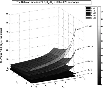
Computing the value of the project for a broad range of values forS, K1 andK2,
we get the following representations. BecauseF : R3 →
Rand one can just have a
clear representation of a function fromR2 → R, we always fixedS = Siand plotted
9All simulations were made on a Mac Mini 2 Core 2 Duo 2.2 GHz using Matlab 7.4.0. Time needed
to run the 15000 events was around 5 minutes. Matlab files are available on demand. Please contact Joachim Gahungu at [email protected] or +32 10 47 94 27.
¯
F(Si, K1, K2)as a function ofK1 andK2. We did it forS= (0, 5, 10, 15, 20)and drawn 5
surfaces on each graph.
Fig. 5: The value of the (2,1) exchange
Fig. 6: The value of the (2,1) exchange
It is decreasing in bothK1andK2as one can see following each surface along the two
axes. It is increasing inSas a higher value ofSleads to a higher position of the surface.
4.4 Conditions on the fundamental quadratic form
Consider now the fundamental quadratic formQ(λ, γ). As a binary quadratic form,
its 0-level curve contains an infinite number of points. Including the conditionγ=ηλ,
the resulting one variable quadratic inλhas two roots.
Q(λ, ηλ) = 1 2λ(λ−1) σ2S+σ2K 1−2ρSK1σSσK1 +λ(µK1−µS) + 1 2ηλ(ηλ−1) σ2S+σ2K 2−2ρSK2σSσK2 +ηλ(µK2−µS) + ηλ2σ2S−ρSK1σSσK1−ρSK2σSσK2+ρK1K2σK1σK2 − (r−µS) (31)
We need to show whether one of this roots has the necessary sign for the Bellman function to make economic sense. We consider the two following problems.
4.4.1 The exchange ofK1+K2forS
The economics of the problem imposes that Bellman function of the (2,1) exchange is
decreasing in bothK1andK2i.e.
F(S, K1, K2) =AS K1 S λ2K2 S γ2 (32)
with bothλ2 andγ2 negative. But λ2 = ηγ2 with η > 0. To make sense, one thus
should determine under what conditions
for allη > 0, Q(λ, ηλ)has a negative rootλ2. (33)
Note that these conditions also ensure that the trigger factor in (29) is greater than one.
4.4.2 The exchange ofSforK1+K2
From the preceding sections, it is clear that the Bellman function of the problem of
exchangingSforK1+K2is F(S, K1, K2) =AS K 1 S λ1K 2 S γ1 (34)
with bothλ1andγ1positive. It leads to the same quadratic form (26) and to (31).
The economics of this problem requires that the Bellman function (34) decreases withSi.e.λ1+γ1 > 1. One should thus determine under what conditions
for allη > 0, Q(λ, ηλ)has a positive rootλ1s.t.λ1(1+η)> 1. (35) As we will see in Section 6, these conditions also warrants that the trigger factor of the (1,2) exchange problem is greater than one.
4.4.3 Conditions on the drift rates
One can not determine analytically under what conditions (33) and (35) hold because the only relation linking the correlation factors is the covariance matrix which is sup-posed to be positive definite. This condition is not easily algebraically handleable.
However, one can show using Monte Carlo simulation that (33) and (35)
simul-taneously hold providing the growth parametersµS,µK1 andµK2 are lower than the
discount rater.11
To summarize, assumingµS,µK1,µK2 < r, the quadratic
Q(λ, ηλ), η > 0
has a positive and a negative root, respectivelyλ1andλ2such that :
1. λ1(η) +γ1(η) = (1+η)λ1(η)> 1
2. λ2(η) +γ2(η) = (1+η)λ2(η)< 0.
5
The (n,m) exchange problem
The dynamic programming approach gives a solution to the general problem of
ex-changing a bundle ofnassets formothers. Noted=n+mas the total dimension of
the problem. We extend the above discussion to obtain a forward investment rule and an expected Bellman function.
Example 2(The (n,m) exchange problem). Assume one is considering the perpetual amer-ican option to pay a sum ofnstochastic sunk costs i.e. a total costa1K1(t) +a2K2(t) +· · · + anKn(t)for a project whose value is a sum ofmstochastic assetsb1S1(t) +b2S2(t) +· · · +
bmSm(t). When is the right time to exercise this option? We extend the above reasoning and proceeds. 1. We first assume no correlation
(a) Solve by multiplicative variable separation and determine the power form. (b) Find the conditions at trigger using the smooth pasting conditions.
(c) Find the homogeneity condition using the value matching condition. (d) Determine the fundamental quadratic form.
2. We then assume correlation
(a) We take the multiplicative power form obtained in (1a) and check that it solves the Bellman differential equation.
(b) On that basis we determine the fundamental quadratic form.
This formal work is left to the Appendix. We just show the general procedure to extract the trigger surface.
The investment trigger has to be ad−1manifold.
For thedassets problem, one has:
11Matlab files available on demand. Please contact Joachim Gahungu at
• one value matching;
• dsmooth pastings; thesedsmooth pastings lead tod−1 conditions at trigger
and one condition for theAcoefficient of the Bellman function.
For given exponents of the Bellman function, the application of thed−1conditions
at trigger reduces the trigger surface(S1(τ), . . . , Kn(τ))from adto a 1-manifold.
It remains to find the admissible set of thedunknown exponents. The value
match-ing condition implies an homogeneity equation, thus reduce the exponents admissible
set from adto ad−1manifold.
Moreover the Bellman function has to be solution of the Bellman differential equa-tion. This implies that the exponents satisfy an equation — the quadratic form — that
reduces this admissible set to ad−2manifold.
The investment trigger is the cartesian product of the 1-manifold for the trigger
surface(S1(τ), . . . , Kn(τ))assuming known exponents by thed−2manifold
describ-ing the allowed exponents. It is ad−1manifold.
Given the trigger manifold, it remains to identify the first exit time. This is done by identifying whether the values of the processes allow one to determine univocally
thedexponents. This requiresd−2additionnal conditions to identify a point of the
d−2admissible manifold. Thesed−2additionnal conditions are given by the values
of the processes at the first exit time. They are called thefiltration matchingrelations.
Referring to the (2,1) exchange problem as an example. This problem has three
state variables. One needs3−2 = 1 other relation coming from observations. This
relation is precisely the value of the parameterη(τ)∈ Fτ.
Usingfiltration matchingconditions, one can solve the(n, m)exchange problem.
Proposition 12 (The solution of the (n,m) exchange problem). Assuming a separable form for the (n,m) exchange problem, the Bellman function of the problem has the power form
F(S1,· · · , Sm, K1,· · · , Kn) =AΠmi=1Sβi i Πnj=1Kλj j with βi> 0,∀i λj < 0,∀j m X i=1 βi+ n X j=1 λj =1.
Moreover, the right time to exercise the (n,m) exchange option is given by
τ=min t | Q(~α) =0 , Xk(t) Xi(t) = αk αi ci ck ∀i,∀k with Q(~α)≡ nX+m i=1 µiαi+1 2 nX+m i=1 nX+m j=1 ρijσij δijαi(αi−1) + (1−δij)αiαj −ρ.
6
Additional problems
This section gives solutions to additional problems. We first treat the (1,2) exchange problem and then take up the (0,2) and the (2,0) exchange problems. The methodol-ogy can be applied to multi-assets irreversible investment. Still, we leave these appli-cations for future work.
Example 3(The (1,2) exchange problem). Consider the perpetual American option to pay a stochastic sunk costsK(t)for a project whose value is the sum of two random assetsS1(t) + S2(t). When is the right time to exercise this option?
The Bellman function of this problem is
F(K, S1, S2) =AK S1 K γ1S2 K λ1 . (36)
For economic reasons, we expectA > 0.γ1andλ1are positive as the Bellman function
must be increasing in bothS1 andS2. The couple(λ1, γ1)belongs to the 0-level curve
of a quadratic formQ0(λ, γ).
One then applies the value matching and smooth pasting conditions for this
problem. The project is continuous at the border between the two regions i.e.
F(K(τ), S1(τ), S2(τ)) =S1(τ) +S2(τ) −K(τ). It must also be smooth at this border then
FS1(K(τ), S1(τ), S2(τ)) = FS2(K(τ), S1(τ), S2(τ)) = 1and FK(K(τ), S1(τ), S2(τ)) = −1. The three smooth pasting conditions lead to two conditions at trigger.
S2(τ) S1(τ) = λ1 γ1 (37) K(τ) S1(τ) = (γ1+λ1−1) γ1 (38)
Note that we showed in Section 4.4 thatγ1 +λ1 > 1provided all the drift rates
lower than the exogeneous discount rate. One pointed out that this condition is of the essence.
Equation (38) is a relation at trigger. At each momenttone measuresS1(t),S2(t)
andK(t). One then uses the information at timetto check if the threshold has been
reached using the standard algorithm. The investment trigger is defined by
T0(2)≡ (S1, S2, K) | S2 S1 = λ1 γ1, K(τ) S1(τ) = (γ1+λ1−1) γ1 , Q(γ1, λ1) =0 .
Using (37), one obtains the intuitive formulation T0(2)≡ (S1, S2, K) | S2 S1 = λ1 γ1, S1+S2 = λ1+γ1 λ1+γ1−1 K, Q(γ1, λ1) =0
and becauseγ1 +λ1 > 1(see Section 4.4), the real options factor is greater than 1 as
expected.
One alternatively uses the value matching or one smooth pasting to determine the coefficientA. A= (γ1+λ1−1) (γ1+λ1−1) γγ1 1 λ λ1 1 (39)
Example 4(The (0,2) exchange problem). Consider the perpetual American option to pay a deterministic sunk costI =K(0)for a project whose value is the sum of two random assets
S1(t) +S2(t). When is the right time to exercise this option?
Intuition suggests to conjecture that the Bellman function of this project is
F(S1, S2) =BI S1 I γ1S2 I λ1
as this would relax the general form of the (1,2) exchange problem. However, such a motivation is not mathematically correct as the differential equation of the (1,2) ex-change problem has one more state variable than the (0,2) exex-change problem. We con-jecture an alternative form of the Bellman function on the basis of variable separation on the (0,2) exchange problem.
The separable solution of the (0,2) exchange problem differential equation is
F(S1, S2) =ASγ1
1 S λ1
2
withγ1andλ1positive andAexpected to be positive after application of the boundary
conditions. Solving the differential equation using this general function holds if the
couple(γ1, λ1) is on the 0-level curve of an easily computed fundamental quadratic
formQ00(γ, λ). One show easily that this special quadratic form is a particular case of
the quadratic of the (1,2) exchange problem withµK = 0andσK= 0. Thus we know
thatλ1+γ1 > 1.
The boundary conditions are the value matchingF(S1(τ), S2(τ)) =S1(τ) +S2(τ) −I
and the two smooth pastingsFS1(S1(τ), S2(τ)) =FS2(S1(τ), S2(τ)) =1.
Solving with the two smooth pasting conditions gives the relation at trigger
γ1 λ1 =
S1(τ)
S2(τ) (40)
and an expression forAin terms of the price processes at triggerS1(τ).
A= 1 γ1Sγ1−1 1 S λ1 2 = 1 γ1(λ1 γ1) λ1Sγ1+λ1−1 1 (41)
As one can not have the usual relationλ1 +γ1 = 1, we remain with two unknown
powers.
Using the value matching condition, relation (41) forAand the relation at trigger
(40), one obtains the investment rule
S1(τ) =
γ1
γ1+λ1−1
I. (42)
One can then use the standard algorithm with the prices ratio at trigger as a source
of information : given the price ratio at timet, one can find the two powersλ1andγ1
and check if the investment criterion (42) holds.
The investment trigger has to verify the set of equations T00(2)≡ (S1, S2, K) | S2 S1 = λ1 γ1, S1(τ) = γ1 γ1+λ1−1 I, Q00(γ1, λ1) =0 .
Using (40), one obtains the intuitive formulation T00(2)≡ (S1, S2, K) | S2 S1 = λ1 γ1, S1+S2 = λ1+γ1 λ1+γ1−1 I, Q00(γ1, λ1) =0
and again note than the real options factor is greater than 1.
One can compute the coefficientA.
A= (λ1+γ1−1) (λ1+γ1−1) λλ1 1 γ γ1 1 I(λ1+γ1−1) = (λ1+γ1−1) (λ1+γ1−1) λλ1 1 γ γ1 1 I(1−λ1−γ1)
We thus fall back on our initial intuition as we can write the general solution of the (0,2) exchange problem as F(S1, S2) =BI S1 I γ1S2 I λ1 with B= (λ1+γ1−1) (λ1+γ1−1) λλ1 1 γ γ1 1 .
Example 5(The (2,0) exchange problem). Consider the perpetual american option to pay the sum of two stochastic sunk costs K1(t) +K2(t) for a project whose value S(0) = V is deterministic. When is the right time to exercise this option?
One can prove that the solution of the problem will take the form
F(K1, K2) =BV K1 V γ2K2 V λ2
with (γ2, λ2) a negative point (i.e. λ2 < 0 andγ2 < 0) of the 0-level curve of the
fundamental quadratic form of the previous problem. The proof is immediate from the preceding example.
7
Conclusion
In this paper, we solve the real option problem of the exchange between n and m
assets using dynamic programming. Our analysis assumes that each asset follows a geometric Brownian motion, and that the exchange option is American and perpet-ual. We are thus in the general framework of real option initiated by Mc Donald and Siegel[11].
We develop the approach on the simple two to one asset exchange that we later ex-tend to the general case. We build up intuition by first considering the case of uncorre-lated risk factors and find a product power form for the solution of the Bellman partial differential equation. We then note that this solution also solves the Bellman partial differential equation of the correlated case. In this process, we derive a quadratic rela-tion that the exponents of the different factors of the product form need to satisfy. We refer to this relation as the fundamental quadratic form.
The fundamental quadratic form, together with the boundary optimality condi-tions define a stopping time that triggers the investment. This is obtained as follows. The value matching condition implies homogenity of degree one of the Bellman func-tion. This is a second condition on the exponents of the Bellman function that re-duces the set of possible exponents to a manifold of dimension 1. The smooth pasting conditions can be reduced to two relations between the three state variables that de-fine a manifold of dimension 1.These relations involve the exponents of the Bellman function. All in all these define a trigger described by a manifold of dimension 2. A 2-dimensional trigger is quite intuitive for a three assets problem.
The Bellman function of the project depends on the value of the assets at the ex-ercise point. In constrast with standard real option problems, the Bellman function cannot therefore be computed ex ante, that is, before the first exit time from the con-tinuation region. We can however compute an ex ante value of the project as an ex-pectation of the Bellman function using Monte Carlo simulation. We show that this expectation also satisfies Bellman partial differential equation.
We show in numerical treatment that the solution of this three assets problem has a good real option behavior. Among other things, the incentive to wait increases with the volatility of every asset.
We then extend this result to thentomexchange problem. Using the same
rea-soning we find a trigger of dimensionm+n−1.
Then we define the key concept of this paper : the filtration matching conditions.
With more than two assets, one has to use the filtration generated by the processes up
to current time. In an+mexchange problem, one needn+m−2conditions coming
from observations.
Additionnal problems are treated as application of the general method.
References
[1] BALDURSSON. Irreversible investment under uncertainty in oligopoly. Journal of
economic dynamics and control(1997).
[2] BERTOLA, G. Irreversible investment.Research in Economics(1998).
[3] BINGHAM, N., AND KIESEL, R. Risk-Neutral Valuation : Pricing and Hedging of
Financial Derivatives. Springer, 2001.
[4] DIXIT, A. K.,AND PINDYCK, R. S. Investment under Uncertainty. Princeton
Uni-versity Press, January 1994.
[5] GRENADIER, S. Option exercice games : an application to the equilibrium
invest-ment strategies of firms. Review of financial studies(2002).
[6] KARATZAS, I., AND BALDURSSON, F. M. Irreversible investment and industry
equilibrium. Finance and stochastics 1(1996), 69–89.
[7] KARATZAS, I.,ANDSHREVE, S. E.Brownian Motion and Stochastic Calculus
(Grad-uate Texts in Mathematics). Springer, August 2004.
[8] KESTER, C. Today’s options for tomorrow’s growth. Harvard Business Review
(1984).
[9] LEAHY, J. Investment in competitive equilibrium : the optimality of myopic
behavior. Quaterly journal of economics(1993).
[10] MARGRABE, W. The value of an option to exchange one asset for another. The
Journal of Finance 33, 1 (1978), 177–186.
[11] MCDONALD, R.,ANDSIEGEL, D. The value of waiting to invest. The Quarterly
Journal of Economics 101, 4 (1986), 707–728.
[12] MYERS, S. Determinants of corporate borrowing. Journal of Financial Economics
[13] OKSENDAL, B. Stochastic Differential Equations. Springer, 2007.
[14] PINDYCK, R. S. Irreversibility, uncertainty, and investment. Journal of economic
literature(1991).
[15] PINDYCK, R. S. Investment of uncertain cost.Journal of Financial Economics(1993).
[16] SHREVE, S. Stochastic Calculus for Finance. Springer, 2005.
[17] SLADE, M. What does an oligopoly maximize? Journal of Industrial Economics
(1994).
[18] WILMOTT, P. Paul Wilmott on Quantitative Finance. Wiley, March 2006.
A
The (1,1) exchange problem
A.1 Proof of Proposition 1
Proof. We assumed a solution
F(S, K) =AK S
K β
.
ReplacingFby this general solution in the differential equation (1) we find thatβmust
be a root of the fundamental quadratic
Q(β)≡ 1 2β(β−1) σ2S+σ2K−2ρSKσPσI +β(µS−µK) − (r−µK).
One still needs to apply the 3 boundary conditions. One notes β1 the positive root
of the fundamental quadratic in the following. At the point (S(τ), K(τ)) where
in-vestment is optimal, one has continuity in the value of the project and "high contact" conditions.
The first condition is the well known value matching
F(S(τ), K(τ)) =S(τ) −K(τ). (43)
At the optimal point the value of the option to wait is just equal to the value of the running project. One gives up the option to wait for a project where its value is at least the sunk cost plus the option to defer. The second and third conditions are the "smooth pasting" conditions.
FK(S(τ), K(τ)) = −1 (44)
FS(S(τ), K(τ)) = 1 (45)
The interpretation of these relations is that if the Bellman function weren’t smooth at the border between the two regions one could do better exercising at an other point.
The application of these conditions leads to
1 A = (β1−1) S(τ) K(τ) β1 1 A =β1 S(τ) K(τ) β1−1 .
The trigger relation between S(τ) and K(τ) makes these two relations actually the
same. One find the condition at trigger
S(τ) = β1 β1−1K(τ)