(will be inserted by the editor)
RER: a Real time Energy efficient Routing protocol for query-based
applications in Wireless Sensor Networks
Ehsan Ahvar · Gyu Myoung Lee · Noel Crespi · Shohreh Ahvar
Received: date / Accepted: date
Abstract Energy-aware routing protocols can be classified into two categories, energy savers and energy balancers. En-ergy saver protocols are used to minimize the overall enEn-ergy consumed by a wireless sensor network (WSN), while en-ergy balancer protocols efficiently distribute the consump-tion of energy throughout the network. Energy saver proto-cols are not necessarily good at balancing energy consump-tion and energy balancer protocols are not always efficient at reducing energy consumption. On the other hand, although delay is another important factor for WSNs energy-aware protocols do not take care of it. This paper proposes a Real time Energy efficient Routing(RER) protocol for query-based applications in WSNs, which offers an efficient trade-off be-tween traditional energy balancing and energy saving objec-tives while supporting a soft real time packet delivery. This is achieved by means of fuzzy sets and learning automata techniques along with zonal broadcasting to decrease total energy consumption.
Keywords Wireless sensor network·Routing protocol· Real time·Energy efficient
Ehsan Ahvar
Institut Mines-Telecom, Telecom SudParis, Evry, France E-mail: [email protected]
Gyu Myoung Lee
Liverpool John Moores University, Liverpool, U.K Tel.:+44 (0)151 231 2052
E-mail: [email protected] Noel Crespi
Institut Mines-Telecom, Telecom SudParis, Evry, France E-mail: [email protected]
Shohreh Ahvar
Institut Mines-Telecom, Telecom SudParis, Evry, France E-mail: [email protected]
1 Introduction
A Wireless Sensor Network (WSN) includes some sensor nodes, which are deployed either inside the phenomenon or very close to it [2]. Basically, each sensor node has capabil-ity of sensing, packet transmission, data processing, mobil-ity, and location finding. However, some of these capabilities can be optional, such as mobility. Sensor nodes can coordi-nate with each other to get high-quality information about the physical environment. These nodes have the ability to communicate amongst each other. They sometimes can di-rectly communicate to an external station.
Because sensors are generally battery-powered nodes, the critical aspects to face concern how to improve the power consumption of sensor nodes, so that the network lifetime can be extended to reasonable time [3]. As the battery car-ried by each mobile sensor node has a limited power supply, computing power is limited, which in turn limits supported services by each node. This restriction is considered as a se-rious challenge in WSNs, where each node has to act as both an end system and a router node at the same time and, there-fore, additional energy is needed to send packets to other nodes.
Many routing algorithms and protocols have been pro-posed for different types of WSNs (i.e., [4, 5], [8–13], [15– 18], [20], [22, 23]) among which we have identified a cat-egory known as query-based routing. For this catcat-egory, a station S sends queries to find specific events among the WSNs. The strategies used for routing these queries and their corresponding replies can be classified into two ma-jor groups, energy savers and energy balancers. The former tries to decrease the energy consumption of the network as a whole and thereby increase the operation lifetime which also usually leads to the utilization of the shortest paths. The lat-ter, on the other hand, tries to balance the energy consump-tion of the nodes to prevent particonsump-tioning of the network.
Rumor is an energy saving protocol that provides an ef-ficient mechanism combining push and pull strategies to ob-tain the desired information from the network [6]. In Rumor, the nodes generating events send notifications that leave a sticky trail along the network. When query agents visit a node where an event notification agent has already passed through, they can find pointers (i.e., the trail) towards the lo-cation of the corresponding source. In general terms, when a node receives a query two things can happen: i) the node already has a route toward the target event, so it only needs to forward the query along the route; or ii) the node does not have a route, and therefore, it forwards the query to a ran-dom neighbor. The ranran-dom selection of the neighbor in this case is relatively constrained, since each node keeps a list of recently visited neighbors to avoid repeatedly visiting them. Clearly, the forwarding strategy in Rumor could end up producing spiral paths, so an intuitive improvement would be to reduce its level of routing indirection. To this end, Cheng-Fu Chou et al. proposed the Straight Line Routing (SLR) protocol [7], which aims at making the routing path grow as straight as possible. More recently, Shokrzadeh et al. made significant efforts to improve Rumor in different as-pects with their Directional Rumor (DRumor) [19]. Shokrzadeh et al. later improved their DRumor protocol by means of what they called the Second Layer Routing (SecondLR) [21]. SecondLR uses geographical routing immediately after lo-cating the source of an event, and Shokrzadeh et al. have shown that this approach considerably improves the perfor-mance of DRumor. Despite these efforts, current query-based routing protocols are mainly energy savers, and have shown relatively poor performance when it comes to balancing en-ergy consumption.
Much more recently, Ahvar et al. have proposed the Energy-aware Query-based Routing protocol (EQR), an energy saver and balancer routing protocol [1]. EQR uses zonal broad-casting to reduce energy consumption.
This paper presents a routing strategy applicable to var-ious forms of query-based applications and offers a reason-able trade-off between the energy and delay objectives. More precisely, we propose a Real time Energy efficient Routing protocol for query-based applications in WSNs called the RER, supported by a learning automata, a fuzzy sets and uses zonal broadcasting to decrease the total energy con-sumed. Our initial results demonstrate the potential and the effectiveness of RER in energy awareness and even in de-lay, making it a promising candidate for a number of WSN applications.
The rest of the paper is organized as follows. In Sec-tion 2, we introduce our design goals. SecSec-tion 3 presents the main contribution of this paper which is basically the RER routing strategy. The assessment of RER is covered in Sec-tion 4, and SecSec-tion 5 concludes the paper.
2 Design Goals
More specifically, RER satisfies the following design objec-tives:
– (1)Energy-distance optimization:Energy-awareness means both energy saver and energy balancer concepts. Energy saver protocols try to decrease the energy consumption of a network to increase network lifespan. They usually try to find the minimum path length to reduce energy consumption. Energy balancer protocols try to balance the energy consumption of nodes to prevent network par-titioning. Finding the best route only based on energy balancing concept may lead to longer paths with greater delay, and finding the best route based only on energy saving concept and optimal distance may lead to net-work partitioning. The RER is an energy saver and an energy balancer at the same time. It achieves a tradeoff between distance and energy by using learning automata and fuzzy sets techniques.
– (2)Accuracy:Finding the best node as a next hop in as-pects of energy saving and balancing is a big challenge for routing protocols. Most energy-aware routing proto-cols find the next hop based on only one measurement factor, such as energy level. The RER, however, consid-ers hop count and distance as well as energy level, si-multaneously, utilizing more than one decision-making technique to achieve more exact results.
– (3)Localized behavior and scalability:The ability to main-tain performance characteristics irrespective of the size of the network is referred to as scalability. Pure localized algorithms are those in which any action invoked by a node should not affect the system as a whole. In these protocols, a node usually uses flooding to discover new paths. In WSNs, where thousands of nodes communi-cate with each other, broadcast storms may result in sig-nificant power consumption and even in a network melt-down. To avoid that situation, most of the distributed op-erations in RER are localized to achieve high scalability. – (4)Soft real time: Although the main goal of the RER is saving and balancing energy, in time-critical situation this protocol can be changed from a pure energy-aware (normal mode) to a delay-aware (critical mode) routing protocol.
– (5)Minimal state architecture:The physical limitations of WSNs, such as large scale, high failure rate, and con-strained memory capacity, demand a minimal state ap-proach. The RER only maintains the immediate neigh-bor’s information and so it does not need a large routing table. Thus, its memory requirements are minimal. – (6)Link failure detection:The RER has the ability to find
a broken link. Unlike most protocols it does not use the Acknowledge packet to check link stability. The RER verifies links by means of the overhearing technique.
– (7)Minimal control packet: In many routing protocols the nodes’ energy levels are forwarded to neighbors by Acknowledge packets. The proposed routing protocol uses the overhearing technique for updating energy lev-els. In most routing protocols, nodes with very low en-ergy levels send a packet to warn their neighbors. The RER instead has a threshold, and when each neighbor forwards a packet, all the neighbors receive it and com-pare the attached energy level of the sender node to the threshold level. If the sender energy is under the thresh-old, the sender is considered to be a dead node and will not be selected again as a next hop. Therefore, the pro-posed protocol does not need an extra packet to announce a dead node. The threshold level is the energy required to send a packet.
– (8)Mobility:Although WSNs usually do not need to con-sider a high degree of mobility but the proposed protocol supports node mobility. Source node can send its query from any place. Our query zone is established on de-mand and dynamically. Also we consider an expected zone specialized for supporting mobility of destination node.
3 Real time Energy efficient Routing (RER)
This section is divided into three main parts. The first part includes some useful definitions and terms that used in our RER protocol. Second part introduces the RER components and the third part gives a brief, general overview of the RER protocol mechanism.
3.1 Definitions
– Def.1:Station. a station or sink node is a node that creates a query packet. In fact, the station is original source of a query packet.
– Def.2:Sender node. each node that sends query or data packet is called a sender node. In fact, a sender node is a previous hop of a packet.
– Def.3:Destination node. a target node that we try to find it by sending query packet is called destination.
– Def.4:Query packet. a query packet is a request packet for receiving information on a particular event.
– Def.5:Data packet. when a destination node or an event witnessed node receives a query packet, it creates a data packet and sends back the packet to the station. A data packet includes information that an event witnessed node or a destination node wants to transfer to the station. – Def.6:Neighbor Table. Neighbor Table is a data
struc-ture that is created inside each node to store information about its one-hop neighbors.
ZEU
EDU
M2: FS
MCUTEU
NUU
Neighbor Table DispatcherDPSU
Decision Maker NM CMM1: LA
PCU PUU API Modes NL NR SL SRFig. 1 RER protocol
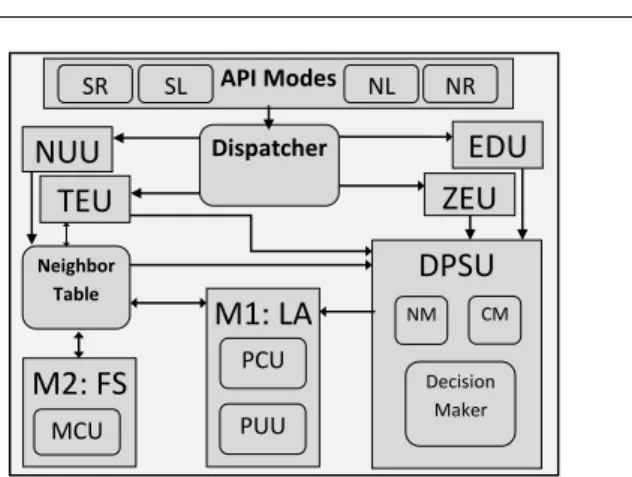
3.2 RER Components
Our proposed RER protocol basically includes following com-ponents:
– (1)an Application Programming Interface (API), – (2)a Dispatcher module,
– (3)a Neighbor Update Unit (NUU), – (4)a Time Estimation Unit (TEU), – (5)a Zone Estimation Unit (ZEU), – (6)a Data Path Selection Unit (DPSU), – (7)a Membership Computation Unit (MCU), – (8)a Probability Computation Unit (PCU), – (9)an Error Detection Unit (EDU) and
– (10)a Probability Update Unit (PUU),(see Fig.1).
For more clarification, we considered two modules: M1:LA module and M2:FS module. The M1:LA module covers all components of learning automata and the M2:FS is a mod-ule related to fuzzy set technique.
In brief, the RER protocol provides four application-level API modes called Non-specific Location (NL), Spe-cific Location (SL), Non-speSpe-cific Region (NR), and SpeSpe-cific Region (SR) for different type of applications. The ZEU is responsible for estimating the query zone. The Dispatcher is a module responsible for receiving piggybacked informa-tion and then transmitting it to the appropriate modules. The NUU gets information from Dispatcher and inserts it into the Neighbor Table. As its name indicates, the EDU is designed to detect errors. The DPSU is the core routing module and hence is responsible for choosing the next hop during the packet forwarding process. The DPSU supports two modes: normal and critical. In normal mode, its Decision Maker (DM) selects an optimum neighbor as the next hop, based on both the membership (from M2 field) degree and the prob-ability (from M1 field) of each neighbor, available in the Neighbor Table (Neighbor Table’s fields will be described in Section 3.2.3). The membership degree associated to each neighbor is computed by the MCU (in the M2:FS module) and the probability of each neighbor is computed by the
PCU and then updated by the PUU (in the M1:LA mod-ule). In critical mode, the TEU alerts the DPSU that there is no enough time to deliver the data packet. Then DPSU trig-gers the immediate selection of the nearest neighbor to the station as the next hop. The constellation of modules is thus mainly designed to assist the DPSU. We describe each unit in detail in the following sub-sections.
3.2.1 Application API and Packet Format
– API modes:As we mentioned the RER protocol supports four application-level API modes: NL, SL, NR and SR. In this architecture, the SR and NR modes are used for event monitoring. The SR is used for applications that monitor events in a specific region of the network, while the NR is used when there is no prior knowledge about where such events occur. In the NR mode, the query packets must be broadcast throughout the entire network to locate potential events.
The two remaining modes, SL and NL, are designed for querying a given node and getting information directly from it: SL when there is prior knowledge about the ex-pected location of the node, and NL when its location is unknown.
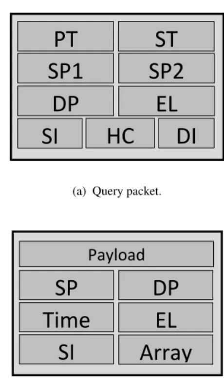
– Query Packet:The query packet contains the following fields: Packet Type (PT), Start Time (ST), Sender Id (SI), Destination Id (DI), Sender Position (SP1), Station Posi-tion (SP2), Hop Count (HC), DestinaPosi-tion PosiPosi-tion (DP) and Energy Level(EL)(see Fig.2(a)).
The PT field indicates the type of communication or mode (SL, SR, NL or NR), ST carries start time of query broadcasting, SI saves the Id of the query-sender node, the destination Id is carried by the DI field in the SL or NL mode’s destination. SP1 and SP2 forward the po-sitions of the sender and the station, respectively, and, if available, DP forwards the position of the destination or the center of requested zone. EL indicates the energy level of the sender node and finally HC holds the number of hops from a query sender node to the station. – Data Packet:There is a single data packet format for the
RER protocol, which contains the following major fields (see Fig.2(b)).
Station Id (SI) which is the destination of the data packet or the Id of the station, Payload, an array with a size of 5 that saves the 5 last previous hops to help the PCU to compute probabilities and also to prevent loops, Energy Level (EL) for forwarding the energy level of the data sender node, and Sender Position (SP) which gives the location of the data sender node as well as the Time and Destination Position (DP) fields that indicate the loca-tion of the destinaloca-tion node at a certain time so that the query zone in the station can be estimated for a future query. Therefore, the station can update and estimate the
position of a destination node more exactly after receiv-ing each data packet from it.
PT
SP2
SP1
EL
DP
DI
SI
ST
HC
(a) Query packet.Payload
DP
SP
EL
Time
Array
SI
(b) Data packet. Fig. 2 RER protocol packet formats.3.2.2 Dispatcher
In the query broadcasting phase, the Dispatcher module will receive information and transmit it to the NUU so it can be inserted into the Neighbor Table. In the response phase, use-ful information is attached (piggybacked) to the data packet. The Dispatcher will receive piggybacked information from data packet and send each part of that information to the ap-propriate module.
3.2.3 Neighbor Update Unit (NUU)
The neighbors’ information will be recorded in a Neigh-bor Table. The components of the NeighNeigh-bor Table for each neighbor are as follows:
– Neighbor ID (NID):Holds the Id of a neighbor;
– Energy Level (EL):Holds the energy level of the sender’s neighbor;
– Hop Count (HC):Holds the number of hops from a neigh-bor to the station;
– Sender Position (SP1):Gives the position of the sender (neighbor) node;
– Station Position(SP2):Indicates the position of the sta-tion;
– Module1(M1):Holds the probability associated with a neighbor as computed by the PCU and updated by the PUU; and
– Module2(M2):Contains the membership degree associ-ated with a neighbor as computed by the fuzzy set tech-nique
The Neighbor Table also has three global fields:
– Start Time (ST):Contains the time that a query packet is sent by the station. The NUU receives the start time from a query packet and inserts it in the ST field. – Time to Reach (TTR): Indicates the estimated time it
takes to reach the station from this node; be computed by the TEU.
– TimeS or time stamp:Holds the actual receiving time of the data packet. The EDU uses this field for error detec-tion.
As mentioned earlier, there are two types of packets: query and data. The fields of each type of packet have been de-scribed in previous sections. After receiving a query packet, the Dispatcher sends the sender Id, energy level, hop count, sender position, and the station position information (also the ST, which will be described subsequently) to the NUU, and then NUU will insert (or update) this data into the Neigh-bor Table.
The TEU computes the time it takes to go from this node to the station (the TTR) and inserts it into the TTR field. The method used by the TEU to compute the TTR is described in Section 3.2.4. The TimeS or the time stamp field refers to the data packet receiving time. The EDU uses this field for error detection.
After receiving a data packet, the Dispatcher transmits the piggybacked energy level of the sender node to the NUU. The NUU then updates the sender node’s energy level in the Neighbor Table.
3.2.4 Time Estimation Unit (TEU)
The TEU works based on two concepts: estimation and com-parison. In the query broadcasting phase, the ST is attached to the query packet. We assume our network is synchro-nized. Each node that receives the query packet will estimate TTR from itself to the station based on the current time (CT) of receiving the query packet and the attached ST time:
T T R=CT −ST. (1)
The TEU saves the TTR into the Neighbor Table. After the query broadcasting phase, each node can estimate how much time it takes to reach to the station from itself. In the
response phase, each data sender node first computes the re-maining time (RT) to reach the station.
RT =Deadline−(CT −ST). (2)
Next, the TEU compares the RT with its TTR, with the condition value of TTR>RT will send an alarm to DPSU. After receiving the alarm, the DPSU will change the condi-tion from normal to critical mode.
3.2.5 Zone Estimation Unit (ZEU)
The ZEU is responsible for estimating the query zone. There are four different states for estimating the zone, based on API modes:
– State 1: the ZEU and the SL mode, – State 2: the ZEU and the SR mode, – State 3: the ZEU and the NL mode, – State 4: the ZEU and the NR mode. Following we will describe each state.
State 1: the ZEU and the SL Mode–The SL mode im-proves the efficiency of our query-based routing algorithm by restricting query flooding to a specified query zone. When the WSN starts its operation for querying a given node and getting information from it, the ZEU in the stationS that will issue the queries will lack any zonal information. There-fore, the query mode used by stationS at the beginning of the operations will typically be NL, which means that the en-tire region is assumed to be the query zone. Once the ZEU starts collecting information, the subsequent queries issued by stationScan be made using the SL modes, thus exploit-ing the advantages of zonal broadcastexploit-ing. The SL mode has two terms, expected zone and query zone, which we de-scribe in the following paragraphs.
Expected zone–Consider a nodeS that needs to find a route to nodeD. Assume that nodeS knows that nodeD was at locationLat timet0, and that the current time ist1.
Then, the expected zone of nodeD, from the viewpoint of nodeSat timet1, is the region that nodeSexpects to
con-tain nodeDat timet1. NodeScan determine the expected
zone based on the knowledge that nodeD was at location Lat timet0 [14]. For instance, if nodeS knows that node Dtravels with average speedvorV elocity, thenSmay as-sume that the expected zone is the circular region of radius v(t1-t0), centered at locationL.
In general, the radius is computed based on following equation:
F =V elocity×(t1−t0) +epsilon. (3)
In the equation,V elocityis the average speed.t1is the
current time andt0 is the time of the previous location of
nodeD. The constantepsilonis used to keep radius non-zero in an immobility status.
If nodeSdoes not know a previous location of nodeD, then nodeScannot reasonably determine the expected zone - in this case, the entire region that may potentially be oc-cupied by the ad hoc network is assumed to be the expected zone [14].
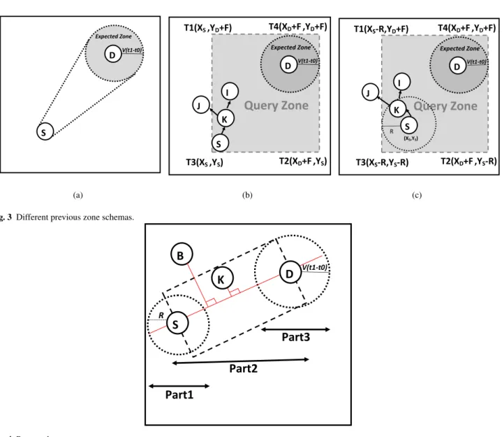
Query zones-After estimating the expected zone, nodeS defines a query zone for the route query. All zonal broadcast-ing algorithms are essentially identical to floodbroadcast-ing, with the modification that a node that is not in the request or query zone does not forward a route request to its neighbors. We describe the previous methods of computing the query zone and then introduce our proposed methods.
Previous query zones- Again, consider nodeSthat needs to determine a route to nodeD. In the LAR1 algorithm, Ko et al. [14] proposed two methods of computing query (re-quest) zones. They proposed a query zone, shown in Fig.3(a), that includes the expected zone. This is not an adequate query zone. All the paths fromStoDmay be located out-side the query zone. Also, this type of zone does not include all the one-hop neighbors of stationS and cannot support acceptable energy balancing in the stationSarea.
Ko et al. also proposed a query zone that is rectangular in shape (Fig.3(b)). Assume that node S knows the aver-age speedV at whichDcan move, and that nodeS knows that nodeD was at location (Xd, Yd) at timet0. Assume
that at time t1, nodeS initiates a new route discovery for
destinationD. Utilizing this knowledge, nodeSdefines the expected zone at timet1to be the circle of radius F = v(t1 -t0) centered at location (Xd, Yd). The query zone is the
rect-angle whose corners areT1,T2,T3andT4. When a node
re-ceives a query, the node discards it if the node is not within the rectangle specified by the four corners included in the route query. For instance, when node j receives the query originally sent from the stationSand forwarded by nodek, it will process the packet but it will not forward it, sincej is not within the query zone delimited by the four corners. Instead, nodesiandkwill process and forward the query, since they are inside the zone determined by the ZEU.
This rectangular zone has the problem as the previous zone: it does not include all the one-hop neighbors of node S and, therefore, energy management and balancing is not possible in the station domain. In a previous study [1], we presented a query zone for balancing energy in the station domain, shown in Fig.3(c). Unlike the method proposed by Ko et al., our proposed method considered all the station neighbors in the zone and can balance energy in the station domain very well.
Our proposed query zones- all the previous methods have one problem in common: zone size. The first zone, pictured in Fig.3(a), is very small and cannot cover enough nodes for effective energy balancing, especially around the station. The other method, shown in Fig.3(b), often covers a vast range of the network as a zone, and the nodes located at the
corners of the zone (near pointsT1andT2) will be useless.
Another visible weakness of Fig.3(b) is all neighbors of the station are not included in the zone and therefore managing energy around station can be so difficult. Although the third zone computing method, Fig.3(c), considers all neighbors of the station in its zone but still its computed zones are of-ten very big and consume more energy. In fact, using these nodes, that are located in the corners of zone, lead to long paths with long delay.
We propose a new query zone with an optimum size. This size optimization can reduce broadcasting query packet transmissions and energy consumption. We also introduce a very simple and efficient method for computing this optimum-size query zone. As Fig.4 shows, we can divide the zone into three parts: part 1, 2 and 3.
– Part.1includes all one-hop neighbors of the station S that are located inside its radio range. Therefore, tech-nically each node that receives a query packet directly from the station considered itself inside the zone. – Part.2can be considered as a rectangular shape. Its length
is equal to distance between our source and destination. For computing its width, first we compute a Threshold. Width of the rectangular shape is considered two times longer than the Threshold. For getting the Threshold, first we compare radio range of the station (radios of part.1) and mobility range of destination (radios of part.3) and after that select the longest as our Threshold. There-fore the Threshold is whether radios of part.1 or part.3. A line that connects source and destination is passing from center of the rectangular shape. This line techni-cally considered as a part.2 zone backbone and all inter-mediate nodes computes their distance from this back-bone. If their distance from the backbone be less than the Threshold they are inside zone.
– Part.3 of zone can be considered as a circular shape. Part.3 covers all possible locations that destination D can be there, we described it before in the Expected Zone and equation (3). Technically each query receiver node computes its distance from destinationD(center of Part.3) and compare it with F in equation(3). If its distance be less thanFit will be inside the zone.
Algorithm.1 shows details of our algorithm for computation of the proposed zone.
State 2: the ZEU and the SR mode–The ZEU acts almost the same way with the SR and SL modes. Instead of the destination location used in the SL mode, the ZEU uses the center position and the radius of the monitored region in the SR mode.
State 3: the ZEU and the NL mode–If the station node does not know the previous location of a destination node,
S D Expected Zone V(t1-t0) (a) S K J I
Query Zone
D Expected Zone V(t1-t0) T4(XD+F,YD+F) T1(XS ,YD+F) T3(XS ,YS) T2(XD+F,YS) (b) T4(XD+F,YD+F) T1(XS-R,YD+F) T3(XS-R,YS-R) T2(XD+F,YS-R) D Expected Zone V(t1-t0) S K J IQuery Zone
(XS,YS) R (c) Fig. 3 Different previous zone schemas.V(t1-t0) R
D
Part1
Part2
Part3
S
B
K
Fig. 4 Proposed query zone
then the station cannot reasonably determine the expected zone. In this case, the entire region that may potentially be occupied by the network is assumed to be the Query zone.
We note that this state occurs only once for each destina-tion node, and that the stadestina-tion will find the posidestina-tion of each node after one query broadcast in NL mode. When the desti-nation node receives the query packet, it includes its current location and current time in the data packet.
When the station receives this data packet, it records the location of the destination node. The station can use this in-formation to determine the query zone for a future query.
State 4: the ZEU and the NR mode–When the station node wants to monitor the network domain to determine if there is an event or not, the entire region that may potentially be occupied by the network is assumed to be the query zone.
3.2.6 Data Path Selector Unit (DPSU)
The constellation of modules is mainly designed to assist the DPSU. The DPSU is the core routing module with the re-sponsibility for choosing the next-hop during the data packet forwarding process. The DPSU can work in one of its two possible transmission modes: Normal and Critical. When the TCU warns the DPSU about shortage of time for deliv-ery current packet, the DPSU will enter its critical mode and select the shortest (hop count) path to reach the station. The TEU is designed to assist the DPSU to select the appropriate mode every time.
If the TCU does not announce any warning, the DPSU will operate in its normal mode. It looks at its Neighbor Ta-ble and finds the neighbor with the highest probability in the M1 field (calledID(M1)) and the neighbor with highest membership degree in the M2 field (calledID(M2)). The highest probability neighbor in the M1 field is a selected
Algorithm 1:The Zone Detector Algorithm
Inputs :{S(XS, YS), D(XD, YD), I(Xi, Yi), R, F}
Output : detecting a node is inside or outside the zone Definition.1:Sis our source or station
Definition.2:Dis our destination
Definition.3:Iis an intermediate node which receive the query Definition.4:Ris radio range of nodeS
Definition.5:Fis radius of expected zone for destination: F=V(t1−t0)
Definition.6: If (F >R) then Threshold=Felse Threshold=R; Definition.7:dis distance between intermediate nodeIand
line passing fromSandDpoints:
d=|(XD−XS)∗(YS−Yi)−(XS−Xi)∗(YD−YS)| [(XD−XS)2+(YD−XS)2]
1 2
.
1 foreachzone detection requestdo
2 ifI am one-hop neighbor of Sthen
3 I am in Part.1 of the zone;
4 else if
((XD> Xi)and(Xi> XS)and(d <=T hreshold))
then
5 I am in Part.2 of the zone;
6 else if
((XD< Xi)and(Xi< XS)and(d <=T hreshold))
then
7 I am in Part.2 of the zone;
8 else if(distance between D and I is shorter thanF)then
9 I am in Part.3 of the zone;
10 else
11 I am not in the zone;
neighbor when using the learning automata technique (the M1:LA module) and the highest membership degree in the M2 field is a selected neighbor by means of the fuzzy set technique (the M2:FS module).
The Decision Maker (DM) will then select the next hop. Note that if the selections made by the M1:LA and M2:FS modules match, then the node selected is chosen as the next-hop. Otherwise, the DM runs a basic sequence of tie-breaking rules until the next-hop is selected.
The processing of the DPSU module is summarized in Algorithm 2. In this algorithm EID(M1) and HID(M1) are the energy level and hop count, respectively, of selected neigh-borID(M1)by means of learning automata andEID(M2)and HID(M2)are the energy level and hop count, respectively, of selected neighborID(M1) by utilizing the fuzzy set tech-nique.
3.2.7 Membership Computer Unit (MCU)
The theory of fuzzy sets was introduced by L. Zadeh in 1965 [24]. Since the pioneering work of Zadeh, there has been a great effort to obtain fuzzy analogues of classical the-ories. Fuzzy set theory is a powerful tool for modeling
un-Algorithm 2:The DPSU Algorithm Input :{ID(M1),E(M1) ID , H (M1) ID } Input :{ID(M2),E(M2) ID , H (M2) ID } Input :{T EU alarm}
Output: next-hop node
1 foreachpacket to be forwardeddo
2 ifReceived alarm from TEUthen
3 Send the packet to nearest neighbor to the station;
4 // If no alarm;
5 else if(ID(M1)==ID(M2))then
6 send the packet to the selected neighbor;
7 // If IDs do not match then run tie-breaking rules;
8 else if(EID(M1)>EID(M2)) && (HID(M1)< HID(M2))
then
9 chooseID(M1)as the next-hop;
10 else if(EID(M1)<EID(M2)) && (HID(M1)> HID(M2))
then
11 chooseID(M2)as the next-hop;
12 elsechoose the one with the highest energy;
certainty and for processing vague or subjective information in mathematical models. Their main directions of develop-ment have been quite diverse and it has been applied to a great variety of real problems. The notion central to fuzzy systems is that truth values (in fuzzy logic) or membership values (in fuzzy sets) are indicated by a value on the range [0, 1], with 0 and 1 representing absolute Falseness and ab-solute Truth, respectively.
The RER algorithm considers a fuzzy set;A. Fuzzy set Aincludes all possible candidates or neighbors. The set also has a membership function. The membership function maps each value (neighbor) to a membership value on the range [0, 1].
Membership function computation–The membership func-tion consists of three factors,K1,K2 andK3, on a range of [0,1]. A fairly efficient way to compute the membership degree of neighbors can be achieved by multiplying these factors together. All three factors of each neighbor will thus be multiplied together to get neighbor’s membership degree. Assume there arenneighbors. Computing of the factors for the membership function of the ith neighbor is described below in more detail:
K1= 1− Hopi M axHop , K2= Energy i M axEnergy , K3= 1− Distancei M axDistance . (4)
The membership degree of theithneighbor can then be computed based on the following function and inserted into theM2field of theithneighbor:
M2=M embershipF unction=K1×K2×K3. (5)
3.2.8 Probability Computation Unit (PCU)
As we mentioned earlier, when a node (i.e., nodei) receives a query packet from a neighbor for the first time (i.e., from neighborK), this produces a new entry in its Neighbor Ta-ble. The Neighbor Table is composed of fields, and each part of the data has to be stored in its related field (described in Section 3.2.3).
The PCU can then compute the probability of neighbor Kfrom the information contained in the Neighbor Table re-ceived from neighborK. The probability Pk(t) associated with neighborKis computed according to the equation (6).
P k(t) = 13 Ek(t) PNi m=1Em(t) + 1 Dk(t) PNi m=1 1 Dm(t) + 1 Hk(t) PNi m=1 1 Hm(t) ! k≤Ni. (6)
As stated above, the probability Pk(t) is computed us-ing the PCU, whereEm(t)is the energy level advertised by neighborm,Ni is the size of nodei’s Neighbor Table (in-cluding now nodek),Dm(t)is the distance advertised by neighbor mto the station S, computed based on equation (7) where (x1,y1) and (x2,y2) are the positions of the station and the current neighbor already saved in Neighbor Table. The sums in the denominators represent the terms to nor-malize the probabilities and to makePNi
k=1Pk(t) = 1.
D= (Y2−Y1)2+ (X2−X1)212. (7)
The rationale of using equation (6) is that it produces a good balance between energy and distance, though at the cost of the potential re-computation of the probabilities im-mediately after each query packet is received, since the sum of the probabilities for all neighbors must be equal to one.
3.2.9 Error Detector Unit (EDU)
As its name indicates, the EDU is designed to detect errors. Most routing protocols use an Acknowledge packet to find if the next hop has received the packet or not. The sender node sends the packet to its next hop and the receiver node sends back an Acknowledge packet. If the sender does not receive
the Acknowledge packet from the receiver, it determines that the link is broken.
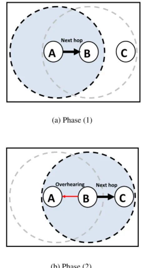
RER does not use an Acknowledge packet. Instead, it verifies links by use of an overhearing technique. For ex-ample, in Fig.5, nodeAsends a data packet toB. WhenB sends the data packet to the next hop, i.e., nodeC, nodeA receives the data packet again via overhearing. If node A does not receive the data packet again after a certain time, it considers the link withBto be broken. In this case, it se-lects another node to send the data. The RER does not need to use an Acknowledge packet, thereby saving more energy than traditional protocols.
3.2.10 Probability Update Unit (PUU)
The basics of the mechanism are illustrated in Fig.5, and it works as follows: The M1:LA module in nodeAoffers the neighbor with the highest probability, from the M1 field of Neighbor Table, as its offered next hop (neighborBin this case), and then it waits for final decision by the DM mod-ule of the DPSU. If the DM selects the same node (nodeB in this case) as a next hop, the DPSU informs the M1:LA module (learning automata) whose offered neighbor was se-lected as a next hop.
A
B
C
Next hop
(a) Phase (1)
A
B
C
Overhearing Next hop
(b) Phase (2)
Fig. 5 Update probability and error detection scheme.
Thus, in fact, the PUU will be enabled if the learning au-tomata (the M1:LA module) and the DM of DPSU select the
same neighbor as a the next hop. When nodeBreceives the data packet, its NUU updates the piggybacked energy level of nodeAin its Neighbor Table and all the other neighbors ofAoverhear the data packet and perform the same updates as B, although they discard the packets immediately after processing them. The routing process continues now with nodeBselecting nodeCas its next hop. WhenBsends the data packet toC, nodeAis the one that overhears the packet sent byB; its NUU thereby updates the energy level of the latter and then its PUU will update probability of nodeB.
The PUU functions based on piggybacking and over-hearing techniques; it can compute and mutually update the probabilities in the Neighbor Tables according to the energy levels, hop count and distances obtained from the neighbors. In the example, if the metrics received from nodeBare acceptable, then nodeBis rewarded by the learning automa-ton inA, and the probability associated toBis increased in nodeA’s Neighbor Table. Otherwise,Bis penalized and its probability is decreased.
In our model, we considered four behavioral cases for rewarding or penalizing a neighborB.
In the first case, the energy-distance-hop relationship is below the average, and thus the learning automata inAwill penalize nodeBwith a factorβ.
where<EA(t)>=PmNi=1Em(t)/Nirepresents the average energy of the neighbors of nodeA, andEB(t)stands for the energy level obtained fromB. Likewise,< DA(t)> repre-sents the average distance of the neighbors ofAto the sta-tionS, whileDB(t)represents the distance toSreported by nodeB.<HA(t)>represents the average hop counts of the neighbors ofAto the stationS, whileHB(t)represents the hop count toSreported by nodeB. In the second case, we consider a lower penalization. The selected penalization is β/2. In the third case, nodeAwill reward nodeBwithα/2. We consider that the best case occurs in the fourth case.
Case1 : EB(t) <EA(t)> + <DA(t)> DB(t) + <HA(t)> HB(t) <3, Case2 : EB(t) <EA(t)> + <DA(t)> DB(t) + <HA(t)> HB(t) = 3, Case3 : 3< EB(t) <EA(t)> + <DA(t)> DB(t) + <HA(t)> HB(t) ≤3.5, Case4 : 3.5< EB(t) <EA(t)> + <DA(t)> DB(t) + <HA(t)> HB(t) . (8)
Reward computation —The reward parameterαis used during the update mechanism in order to grant more priority to the nodes giving them more possibilities to forward the response packets to the station. The value ofαis computed using: α=λα+δα E B(t) <EA(t)> ×<DA(t)> DB(t) ×<HA(t)> HB(t) , (9)
whereλαis the minimum reward granted to a well-positioned node, andδαis the limiting factor for the reward.
Penalty computation —Similarly, we use:
β=λβ+δβ E B(t) <EA(t)> ×<DA(t)> DB(t) ×<HA(t)> HB(t) −1 , (10)
where analogously to the reward mechanism,λβis the mini-mum penalty, andδβis the limiting factor. Note that in equa-tion (9) and (10), the better (or worse) the energy–distance relationship the greater the reward (or penalization) assigned for nodeB.
Upon obtaining the energy and distance metrics from node B, the learning automata in nodeA will update the probabilities of its NA neighbors based on equations (11) and (12).
The former applies for the rewarding cases, i.e., the third and fourth cases described above, withxα=α/2andxα= α, respectively. The latter corresponds to the penalization cases, that is, the first and second cases, withxβ =β and xβ =β/2, respectively. PB(tn+1) =PB(tn) +xα[1−PB(tn)] Pk(tn+1) = (1−xα)Pk(tn) ∀k|k6=B∧k≤NA, (11) PB(tn+1) = (1−xβ)PB(tn) Pk(tn+1) = xβ NA−1 + (1−xβ)Pk(tn) ∀k|k6=B∧k≤NA. (12) 3.3 RER Mechanism
RER is an energy-aware routing protocol designed to con-sider packet delivery delay while routing packets across a network. RER balances the load among the different sensors with a twofold goal: preventing the sensors from running out of battery while keeping the routes to reach the destinations relatively short. It also offers a soft real time system. RER can be divided into two phases: query broadcasting and data forwarding.
RER: a Real time Energy efficient Routing protocol for query-based applications in Wireless Sensor Networks 11 v (a) (b)
Query Zone
K S D BQuery Zone
K S D B(a) Query broadcasting phase.
(a) (b)
Query Zone
K S D BQuery Zone
K S D(b) Data forwarding phase. Fig. 6 RER phases.
– Query broadcasting phase —When the WSN starts its operation, a ZEU in the station S that will issue the queries will have no zonal information. Therefore, the query modes used by stationS at the beginning of the operations will typically be NL or NR, which means that the entire region is assumed to be the query zone. Once the ZEU starts collecting information, the subse-quent queries issued by the stationScan be made using the SR or the SL modes, thus exploiting the advantages of zonal broadcasting.
In general terms, stationS will gather zonal informa-tion in its ZEU, and whenever required it will generate a query packet in which it will broadcast some items such as its ID, the query mode (NR, NL, SR, or SL), its po-sition, the zone information, and optionally, the destina-tion ID. The nodes receiving the query packet can for-ward or discard it depending on their location.
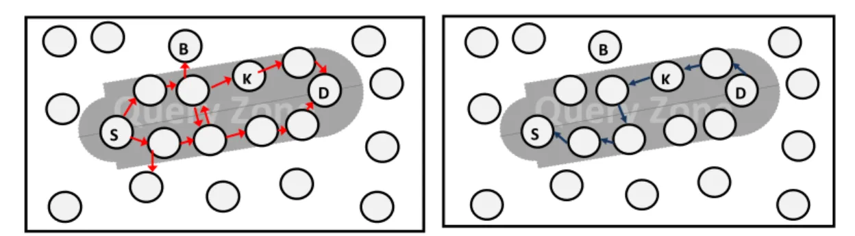
For instance, on the Fig. 6(a), when nodeBreceives the query originally sent from stationS, it will process the packet but it will not forward it, sinceBis not within the query zone. Instead, nodeK will process and forward the query given that it is inside the zone determined by the ZEU.
In brief, the nodes within the query zone distribute the queries complementing the information originally sent by the stationS with their own Id, their energy level, the procedure start time, their position, hop count, dis-tance to the station, and a list of hops to prevent forward-ing loops. This process is repeated until a destination is found.
– Data forwarding phase —When the destination or event witness node receives the query packet, it replies by send-ing a data packet. At this point, every node in the zone knows the energy levels of their neighbors and the dis-tance and hop count from them to the stationS. As shown in Fig.6(b), the response to the station could use a different path, since this will depend on the pri-mary neighbor selected by the DPSU.
4 Performance Evaluation
In this section, we evaluate the RER’s performance by com-paring it to the following routing protocols: Rumor [6], as a basic query-based routing protocol, and EQR [1], as a new query-based routing protocol. To this end, we used the Glo-MoSim simulator developed by UCLA [25]. The simulation model used and the results we obtained with it are described below.
4.1 Simulation Model
We used a surface that was1000m×1000m. The radio range was set to177 m, with an available bandwidth of2
Mbps and a radio transmission(TX) power of4dBm. Each simulation had a 4-hour duration, and the tests were run un-der various conditions, such as with different amount of sen-sors, namely,1000,1200, and1400nodes, and also with 10 different amounts of seeds. Moreover, the placement of the sensors in the terrain and their initial energy levels were se-lected randomly. It is worth highlighting that, even though the placement and initial energy of the nodes were set ran-domly, once set those factors remained fixed for rest of the trials to obtain comparable results across experiments.
In the simulations presented here, the traffic in the net-work is always initiated by a source stationS, which period-ically acquires information from a particular sensord. The sensordmoves at a speed of 40 Metre/Hour. Once the query is received atd, the sensor will immediately send back the response toSwith the requested information.
Scenario I—In this scenario, we assume a critical situation, where the energy levels for transmission mode are very low. Under these conditions, we evaluate the different routing schemes considering three different tests:
– Test 1: Time until the first node runs out of battery power— This test is one of the indicators of the effectiveness of the routing schemes in terms of energy management. In general, those with the capacity to balance the energy consumed should last longer without node failure.
1000 1200 1400 0 2000 4000 6000 8000 10000
Node Number
Time[s]
REC EQR Rumor RER
(a)Test1:Time until the first node runs out of battery. 1000 1200 1400 0 20 40 60 80 100
Node Number
Active Nodes (%)
REC
EQR
Rumor
RER
(b)Test2:Fraction of active nodes.
1000 1200 1400
0
20
40
60
80
100
Node Number
Active Neighbors(%)
REC
EQR
Rumor
RER
(c)Test3:Fraction of active neighbors of S.
Fig. 7 Tests results for Scenario I.
1000 1200 1400
0
100
200
300
Node Number
Transmissions
REC
EQR
Rumor
RER
(a)Test4:Average data packet transmis-sion.
1000 1200 1400
0
2
4
6
x 10
−7Node Number
Variance
REC
EQR
Rumor
RER
(b)Test5:Variance.1000 1200 1400
0
3
5
x 10
−4Node Number
Energy[mW]
REC
EQR
Rumor
RER
(c)Test6:Average energy consumption.
Fig. 8 Tests results for Scenario II.
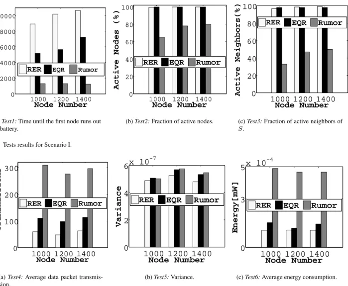
– Test 2: Fraction of active nodes at the end of the simulation— This test gets the total number of sensors that are active (alive) for each routing scheme during a simulation pe-riod of 2 hours, providing an indicator of the capacity of the routing schemes for saving energy. Those protocols with ability of balancing the energy consumed should have lower number of node failure than the others. – Test 3: Fraction of active neighbors of the stationS at
the end of the simulation—Traffic load around station is very heavy because a station is source of the query packets and destination of the data packets. Therefore, managing energy of the station neighbors and keeping the station connected to network is very important. This test shows the ability of the different routing schemes to keep the stationS connected. As in the case ofTest 2, the simulation period for this test is 2 hours.
Scenario II—In this scenario, the energy levels of the sen-sors are set sufficiently high so as to avoid experiencing node failures during the simulation runtime. Our goal in this case
is to compare the fairness in terms of energy consumption. In order to avoid bias in the comparison, we ensure that all the routing schemes transmit the same amount of data, and that this occurs without node failures. We carry out three tests to examine how the routing schemes save and manage energy in regular operation mode.
– Test 4: Average data packet transmission—This test com-putes average number of hops that a data packet should travel to reach to the station for each protocol. It pro-vides another indicator of which routing scheme is more efficient in saving energy.
– Test 5: Variance in the remaining energy levels for the neighbors of stationS—This test considers one-hop neigh-bors of the station and computes a variance in energy level for them. It allows us to examine which routing scheme is the best at performing energy balancing among the nodes close to the station.
– Test 6: Average energy consumption—This test computes average energy consumption of a node for each protocol.
L1
L2
L3
400
500
600
700
800
Deadlines
Time[mSec]
(a)Test7:Ene-to-end delay.
L1
L2
L3
1.05
1.1
1.15
1.2
1.25
x 10
−4Deadlines
Energy[mW]
1.05 1.05 1.15 1.15 1.25X(b)Test8:Average energy consumption.
L1
L2
L3
0
2
4
6
x 10
−7Deadlines
Variance
(c)Test9:Variance. Fig. 9 Tests results for Scenario III.It provides another indicator of which routing scheme is more efficient in managing energy.
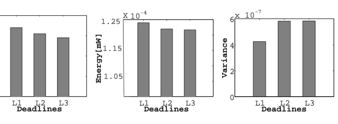
Scenario III—In this scenario, we consider three different levels of deadline: L1(long), L2(medium), L3(short).
We also carry out three tests to examine how the RER protocol can react to these different types of time constraints. – Test 7: Average end-to-end delay—This test shows how
RER can adapt itself to different deadlines.
– Test 8: Average energy consumption—This test shows how energy consumption is changed based on different deadlines.
– Test 9: Variance in the remaining energy levels for the neighbors of stationS—This test identifies which dead-line level produces better energy balancing among the nodes close to the station.
4.2 Simulation Results
Scenario I—The most commonly used measure of network lifetime is the time until the first node runs out of battery energy. In RER the first sensor fails after ∼ 8000 to ∼
11000 seconds depending on the number of nodes present in the network(see Fig. 7(a)). The time in which the first node runs out of battery is relatively shorter for EQR (fails after∼ 5000to∼ 7000seconds) and significantly shorter for Rumor that fails around1000seconds. Fig.7(b) is a good indicator for evaluating energy management of protocols. While Fig.7(b) shows ability of energy management in the network Fig.7(c) specialized to show energy management of protocols only around the station node. Fig.7(b) and Fig.7(c) show that the RER is much better than the more traditional Rumor and that it is relatively similar to the new EQR pro-tocol. In brief, considering the three parts of Fig.7, even though in low battery situations there is no big difference between EQR and RER in terms of the number of node
fail-ures, it is clear RER can keep a network alive longer than EQR.
Scenario II—We evaluate these protocols in normal energy situations.
Fig.8(a) shows average number of hops that a data packet should travel to reach to the station for each protocol. The Rumor is the worst routing protocol, mostly because Ru-mor selects its next hops randomly. EQR selects next hops based on learning automata and RER selects them based on both fuzzy set and learning automata. It is clear that selec-tions based on chance (Rumor) leads to a higher number of transmissions than a systematic selection process (EQR and RER). A higher number of transmissions also should con-sume more energy (see Fig.8(c)). One more important point that we can extract from Fig.8(b) and Fig.8(c) together is the RER not only is an energy saver protocol but also it is an energy balancer routing protocol.
Actually, beyond merely comparing the particular values obtained in each figure, the most important conclusions that can be extracted from Fig.8(a), Fig.8(b) and Fig.8(c) as a whole are basically the following. The results show that the combination of a fuzzy set technique and learning automata can improve energy balancing, and more importantly, that the combined operation (RER’s use of fuzzy set plus learn-ing) can work better than only one technique(EQR). Our new proposed zone could also reduce the number of packet transmission and save more energy than previous versions. Scenario III—As mentioned above, RER also acts as a delay-aware routing protocol. Fig.9 (a) shows how RER sets its end-to-end delay based on different deadlines. L1 is a long period deadline and so RER does not receive any alarm from its TEU. Therefore, the DPSU acts in its normal mode and selects its next hops based on energy and distance factors. Therefore, as Fig.9 (c) shows we have the best energy bal-ancing by using L1. However, with the L3 deadline, there is no time to deliver data packet to the station and so that TEU sends an alarm to the DPSU to select the closest neighbor
to the station. In L3 the most important factor is time and therefore a shortest path is selected. By selecting the short-est possible path and reducing number of hops in L3, we expect and also Fig.9(b) shows that energy consumption is reduced in comparison with L1. Selecting the shortest path to reduce end-to-end delay causes increasing variance of L3 in comparison with L1 (Fig.9(c)).
Generally, results of the Scenario.III showed that the RER is a flexible protocol and can adapt itself with different dead-lines and time constraints.
5 Conclusion
In this paper we studied energy-aware query-based routing protocols. From the routing perspective, we have observed that the current destination-initiated query-based routing pro-tocols can be considerably improved, especially, if we aim for a better balance between the energy savings and energy balancing objectives. We have proposed a new real-time en-ergy saver/balancer routing protocol. We simulated and com-pared our routing protocol with traditional Rumor and newer EQR protocols. Indeed, nine different types of tests were carried out and described, and in most of these tests indi-cated that the RER obtained significantly better results.
Acknowledgements This work was supported by the EU ITEA 2 Project: 11012 “ICARE: Innovative Cloud Architecture for Real Entertainment”.
References
1. Ehsan Ahvar, Rene Serral-Gracia, Eva Marin-Tordera, Xavier Masip-Bruin, Marcelo Yannuzzi, EQR: A New Energy-Aware Query-Based Routing Protocol for Wireless Sensor Networks. in Proc. of IFIP WWIC 2012, pp. 102-113, Santorini, Greece, June 2012.
2. Ian F. Akyildiz, Weilian Su, Yogesh Sankarasubramaniam, Erdal Cayirci, Wireless sensor networks: a survey. Elsevier Computer Net-works, Volume 38, Number 4, pp. 393-422, March 2002.
3. Giuseppe Anastasi, Marco Conti, Mario Di Francesco, Andrea Pas-sarella, Energy conservation in wireless sensor networks: A survey, Elsevier Ad Hoc Networks, Volume 7, Number 3, pp.537−568, May 2009.
4. Claudia J. Barenco Abbas, Ricardo Gonzalez, Nelson Cardenas, L. Javier Garcia-Villalba: A proposal of a wireless sensor network rout-ing protocol. Telecommunication Systems journal, pp. 61-68, Vol-ume 38, Numbers 1-2, June 2008.
5. Julio Barbancho, Carlos Leon, Francisco Javier Molina, Antonio Barbancho, A new QoS routing algorithm based on self-organizing maps for wireless sensor networks. Telecommunication Systems journal, pp. 73-83, Volume 36, Numbers 1-3, November 2007. 6. David Braginsky, Deborah Estrin, Rumor Routing Algorithm for
Sensor Networks, in Proceedings of the First ACM Workshop on Sensor Networks and Applications, pp. 22-31, Atlanta, GA, USA, 2002.
7. Cheng-Fu Chou, Jia-Jang Su, Chao-Yu Chen, Straight Line Routing for Wireless Sensor Networks, 10th IEEE Symposium on Computers and Communications, pp. 110-115, Murcia, Spain, 2005.
8. Yuh-Shyan Chen and Yun-Wei Lin, Mobicast Routing Protocol for Underwater Sensor Networks, IEEE Sensors Journal, Volume 13, Number 2, February 2013.
9. Xiao Chen, Zanxun Dai, Wenzhong Li, Yuefei Hu, Jie Wu, Hongchi Shi, and Sanglu Lu, ProHet: A Probabilistic Routing Protocol with Assured Delivery Rate in Wireless Heterogeneous Sensor Networks, IEEE Transactions on Wireless Communications, volume 12, issue 4, pp.1524−1531, 2013.
10. Yuh-Shyan Chen, Yi-Jiun Liao, Yun-Wei Lin, Ge-Ming Chiu, HVE-mobicast: a hierarchical-variant-egg-based mobicast routing protocol for wireless sensornets. Telecommunication Systems jour-nal, Volume 41, Number 1, pp.121-140, May 2009.
11. Junyoung Heo, Jiman Hong, Yookun Cho, Earq: Energy aware routing for realtime and reliable communication in wireless indus-trial sensor networks, IEEE Transactions on Indusindus-trial Informatics, volume 5, number 1, pp.3-11, 2009.
12. Pei Huang, Chen Wang, Li Xiao: Improving End-to-End Rout-ing Performance of Greedy ForwardRout-ing in Sensor Networks, IEEE Transactions on Parallel and Distributed Systems, Volume 23, pp. 556-563, 2012.
13. Xiaoxia Huang, Hongqiang Zhai, Yuguang Fang, Robust coop-erative routing protocol in mobile wireless sensor networks, IEEE Transactions on Wireless Communications, volume 7, number 12, pp.5278-5285, 2008.
14. Young-Bae Ko, Nitin H. Vaidya, Location-Aided Routing (LAR) in Mobile Ad Hoc Networks, Wireless Networks journal, Volume 6, Number 4, pp. 307-321, September 2000.
15. Daichi Kominami, Masashi Sugano, Masayuki Murata, Takaaki Hatauchi: Controlled and self-organized routing for large-scale wire-less sensor networks,ACM Transactions on Sensor Networks, Vol-ume 10, 2013.
16. Soonmok Kwon, Jongmin Shin, Jae Hoon Ko, Cheeha Kim, Dis-tributed and localized construction of routing structure for sensor data gathering. Telecommunication Systems journal, pp. 135-147, Volume 44, Numbers 1-2, June 2010.
17. Antonio Manuel Ortiz, Fernando Royo, Teresa Olivares, Jos Car-los Castillo, Luis Orozco-Barbosa, Pedro Jos Marron: Fuzzy-logic based routing for dense wireless sensor networks. Telecommunica-tion Systems journal, pp. 2687-2697, Volume 52, Number 1, January 2013.
18. XuFei Mao, ShaoJie Tang, XiaoHua Xu, Xiang-Yang Li, Huadong Ma, Energy-efficient opportunistic routing in wireless sensor net-works, IEEE Transactions on Parallel and Distributed Systems, vol-ume 22, number 11, pp.1934−1942, November. 2011.
19. Hamid Shokrzadeh, Abolfazl Toroghi Haghighat, Farzad Tashtar-ian, and A. Nayebi, Directional Rumor Routing in Wireless Sensor Networks, 3rd IEEE/IFIP International Conference in Central Asia on Internet, Tashkent, Uzbekistan, September 2007.
20. Lei Shu, Yan Zhang, Laurence Tianruo Yang, Yu Wang, Man-fred Hauswirth, Naixue Xiong, TPGF: geographic routing in wire-less multimedia sensor networks. Telecommunication Systems jour-nal, pp. 79-95, Volume 44, Numbers 1-2, June 2010.
21. Hamid Shokrzadeh, Abolfazl Toroghi Haghighat, Abbas Nayebi, New Routing Framework Base on Rumor Routing in Wireless Sensor Networks, Computer Communications Journal, Elsevier, volume 32, January 2009.
22. Xiumin Wang, Jianping Wang, Kejie Lu, Yinlong Xu: GKAR: A Novel Geographic(K)-Anycast Routing for Wireless Sensor Net-works, IEEE Transactions on Parallel and Distributed Systems, Vol-ume 24, pp. 916-925, 2013
23. Bernd-Ludwig Wenning, Dirk Pesch, Andreas Timm-Giel, Carmelita Gorg, Environmental monitoring aware routing: mak-ing environmental sensor networks more robust. Telecommunication Systems journal, pp. 3-11, Volume 43, Numbers 1-2, February 2010. 24. L.A.Zadeh, Fuzzy Sets, Inform. Control 8, pp.338−353, 1965. 25. GloMoSim Simulator: http://pcl.cs.ucla.edu/projects/glomosim.
Ehsan Ahvar received a Master degree in computer systems archi-tecture from Azad University of Arak, Iran in 2007. He is currently pursuing his Ph.D at the Institut Mines-Telecom, Telecom SudParis and Paris.VI University (UPMC), France. He was faculty member of Information Technology depart-ment at Payame Noor University (P.N.U), Iran from 2007 to 2012. His research interests include im-proving energy and Quality of Ser-vice (QoS) for wireless sensor net-works, Internet of Things, indoor localization and improving cost for cloud-based applications.
Gyu Myoung Leereceived his BS degree from Hong Ik University, Seoul, Korea, in 1999 and his MS and PhD degrees from the Ko-rea Advanced Institute of Science and Technology (KAIST), Dae-jeon, Korea, in 2000 and 2007.He is with the Liverpool John Moores University (LJMU), UK, as a Se-nior Lecturer in 2014 and with KAIST Institute for IT conver-gence, Korea, as an adjunct pro-fessor from 2012. Prior to join-ing the LJMU, he has worked with the Institut Mines-Telecom, Tele-com SudParis, France, from 2008. Until 2012, he had been invited to work with the Electronics and Telecommunications Research Institute (ETRI), Korea. He also worked as a research professor in KAIST, Ko-rea and as a guest researcher in National Institute of Standards and Technology (NIST), USA, in 2007.His research interests include In-ternet of things, future networks, multimedia services, and energy sav-ing technologies includsav-ing smart grids. He has been actively worksav-ing for standardization in ITU-T, IETF and oneM2M, etc., and currently serves as the Rapporteur of Q11/13 and Q16/13 as well as an Editor in ITU-T. He is a Senior Member of IEEE.
Noel Crespi holds a Master’s from the Universities of Orsay and Kent, a diplome d’ingenieur from Tele-com ParisTech, and a Ph.D. and a Habilitation from Paris.VI Univer-sity. He worked from 1993 in CLIP, Bouygues Telecom, France Tele-comR and Din 1995, and Nor-tel Networks in 1999. He joined In-stitut Mines-Telecom in 2002 and is currently professor and program director, leading the Service Archi-tecture Laboratory. He is appointed as coordinator for the standardiza-tion activities in ETSI and 3GPP. He is also a visiting professor at
the Asian Institute of Technology and is on the four-person Scientific Advisory Board of FTW, Austria. His current research interests are in service architectures, P2P service overlays, future Internet, and Web-NGN convergence. He is the au-thor/coauthor of more than 230 papers and contributions in standard-ization.
Shohreh Ahvar received B.S degree in Information Technology and M.S degree in Electrical Engineering-Telecommunication (Networks) both from Isfahan University of Technology, Isfahan, Iran. She is currently a Ph.D candi-date at the Institut Mines-Telecom, Telecom SudParis, France. Her research interests include improv-ing energy and Quality of Service (QoS) for wireless sensor and ad hoc networks, routing protocols, traffic engineering and analyti-cal evaluation and performance modeling of computer networks and improving cost and QoS for cloud-based applications.