Research Article Global Hopf Bifurcation Analysis for a Time-Delayed Model of Asset Prices

(1)

Discrete Dynamics in Nature and Society Volume 2010, Article ID 432821,17pages doi:10.1155/2010/432821

Research Article

Global Hopf Bifurcation Analysis for

a Time-Delayed Model of Asset Prices

Ying Qu and Junjie Wei

Department of Mathematics, Harbin Institute of Technology, Harbin 150001, China

Correspondence should be addressed to Junjie Wei,[email protected]

Received 7 October 2009; Accepted 13 January 2010 Academic Editor: Xuezhong He

Copyrightq2010 Y. Qu and J. Wei. This is an open access article distributed under the Creative Commons Attribution License, which permits unrestricted use, distribution, and reproduction in any medium, provided the original work is properly cited.

A time-delayed model of speculative asset markets is investigated to discuss the eﬀect of time delay and market fraction of the fundamentalists on the dynamics of asset prices. It proves that a sequence of Hopf bifurcations occurs at the positive equilibriumv, the fundamental price of the asset, as the parameters vary. The direction of the Hopf bifurcations and the stability of the bifurcating periodic solutions are determined using normal form method and center manifold theory. Global existence of periodic solutions is established combining a global Hopf bifurcation theorem with a Bendixson’s criterion for higher-dimensional ordinary diﬀerential equations.

1. Introduction

Efficient Market Hypothesis EMH is a standard theory of financial market dynamics. According to the theory, asset prices follow a geometric Brownian motion representing the fundamental value of the asset, and hence asset prices cannot deviate from their fundamental values. The EMH theory, however, cannot explain excess volatility of financial markets such as speculative booms followed by severe crashes. Recently, models have been developed to explain fluctuations in financial markets see1–9 and the references therein. In such models, asset prices follow deterministic paths that can deviate from fundamental values generating what is called a speculative bubble in asset markets. In speculative markets modeling, almost all the previous models have utilized either differential or difference equations methodology.

Dibeh 4 presents a delay-diﬀerential equation to describe the dynamics of asset prices. The author divides market participants into chartists and fundamentalists. The fundamentalists follow the EMH theory and base their demand formation on the diﬀerence between the actual price of the assetpand the fundamental price of the assetv. The chartists, on the other hand, base their decisions of market participation on the price trend of the asset.

(2)

They attempt to exploit the information of past prices to make their decisions of purchasing or selling the asset. In4, the model describing the time evolution of the asset price is given by

dp

dtt 1−mtanh

pt−pt−τpt−mpt−vpt, P

wherem∈0,1is the market fraction of the fundamentalists. A time delay is introduced for chartists since they base their estimation of the slope of the asset price trend on an adaptive process that takes into account past values of the slope of the price trend.

In4, it is shown by simulation that there may exist limit cycles forP, explaining the persistence of deviations from fundamental values in speculative markets. The aim of the present paper is to provide a detailed theoretical analysis of this phenomenon from the bifurcation point of view. Applying the local Hopf bifurcation theory see 10, we investigate the existence of periodic oscillations forP, which depends both on time delayτ

and the market fraction of the fundamentalistsm. Using the normal form theory and center manifold theorem11,12, we derive suﬃcient conditions for determining the direction of Hopf bifurcation and the stability of the bifurcating periodic solutions. Furthermore, taking

τ as a parameter, we establish the existence of periodic solutions forτ far away from the Hopf bifurcation values using a global Hopf bifurcation result of Wusee13and also14–

18. A key step in establishing the global extension of the local Hopf branch at the first critical valueτ τ0is to verify thatPhas no nonconstant periodic solutions of period 4τ.

This is accomplished by applying a higher-dimensional Bendixson’s criterion for ordinary diﬀerential equations given by Li and Muldowney19.

The rest of this paper is organized as follows: in Section2, our main results are stated and some numerical simulations are carried out to illustrate the analytic results. In Section3, results on stability and bifurcations at positive equilibrium are proved, taking m and τ

as parameters, respectively. In Section 4, a theorem on the direction and stability of Hopf bifurcation is provided. Finally, a global Hopf bifurcation theorem is proved.

2. Main Results

Given the nonnegative initial condition

pt ϕ≥0, ϕ0>0, t∈−τ,0, 2.1 EquationPadmits a unique solutionHale and Lunel10. Any solutionpt, ϕofPis nonnegative if and only ifϕ0>0, following the fact that

pt ϕ0et01−mtanhps−ps−τ−mps−vds. 2.2 Note that dp dtt≤ 1−m mv−mptpt. 2.3

(3)

We conclude that, for any suﬃciently small >0,

pt< 1−m

m v 2.4

holds for all larget >0. This establishes the ultimate uniform boundedness of solutions for

P.

EquationPhas two equilibria 0 andv. Denote byp∗any of the equilibria. Then the linearization ofPatp∗is given by

dp

dtt

1−3mp∗ mvpt−1−mp∗pt−τ. 2.5 Ifp∗0, then it is unstable since2.5becomes

dp

dtt mvpt. 2.6

Ifp∗v, then the characteristic equation of2.5is

Δλ:λ−1−2mv 1−mve−λτ 0. 2.7 We investigate the dependence of local dynamics ofPon parametersmandτ.

Case 1. Choosingmas parameter.

Define mk1− 1 2−cosηkτ , 2.8 whereηksolves 2−cosητη−vsinητ0, 2.9

with the assumption ofvτ >1.

Proposition 2.1. Ifm1, thenp∗vis globally stable.

The case of m 1 represents that asset prices are totally determined by the fundamentalists. Obviously, asset prices cannot deviate from their fundamental values v

since the fundamentalists obey the EMH theory.

Theorem 2.2. Assumevτ >1. Then

ithe positive equilibriump∗ vof Pis asymptotically stable whenm ∈m0,1, where

m0:max{mk};

(4)

Case 2. Regardingτas parameter. Define τj 1 ω0 arccos1−2m 1−m 2jπ , j0,1,2, . . . 2.10 withω0 :v m2−3m. Theorem 2.3. ForP,

iifm∈2/3,1, thenp∗vis asymptotically stable for allτ ∈R ;

iiifm∈0,2/3, thenp∗vis asymptotically stable when 0< τ < τ0and becomes unstable

when τ > τ0; moreover,Pundergoes a Hopf bifurcation atp∗ vwhen τ τj j

0,1,2, . . ..

Theorem 2.4gives the direction of Hopf bifurcation and stability of the bifurcating periodic solutions. Similar results hold if we choosemas parameter.

Theorem 2.4. Assumem∈0,2/3. If Rec10<0>0, then the bifurcating periodic solutions

atv are asymptotically stable (unstable) on the center manifold and the direction of bifurcation is

forward (backward). In particular, the bifurcating periodic solution from the first bifurcation value

τ τ0is stable (unstable) in the phase space if Rec10<0>0.

Corollary 2.5. Whenτ τ0,vis stable (unstable) if Rec10<0>0.

Remark 2.6. See the proof in Section 4 for the explanation of c10 which appears in

Theorem2.4and Corollary2.5.

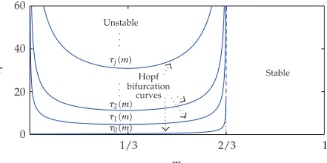
The conclusions above are illustrated in Figure1, using bifurcation set on them, τ-plane. Here,τ0m, τ1m, τ2m, . . . , τjm, . . .are Hopf bifurcation curves. When

m, τ∈D : m, τ|0< m < 2 3,0≤τ < τ0m ∪ m, τ| 2 3 ≤m <1 , 2.11

p∗vis asymptotically stable, and when

m, τ∈Dc: m, τ|0< m < 2 3, τ > τ0m , 2.12

p∗ vis unstable. Denote the curveτ τ0mbyl. Clearly,llies in the boundary ofD. The stability ofvwhenm, τ∈lis given by Corollary2.5.

The occurrence of Hopf bifurcation explains the persistent deviation of the asset price from the fundamental value and it depends both on the time delay and the market fraction of the fundamentalists. In fact, choosing the same parameters as in4, Figure 2:

m0.62, v5, τ2, 2.13 we compute by 2.10 that τ0 1.5304. Therefore, Theorem 2.3 provides insight on the

(5)

0 20 40 60 τ 1/3 2/3 1 m Stable Hopf bifurcation curves τ0m τ1m τ2m . . . τjm . . . Unstable

Figure 1: Hopf bifurcation set onm−τplane.

Finally, a natural question is that if the bifurcating periodic solutions ofPexist when

τis far away from critical values? In the following theorem, we obtain the global continuation of periodic solutions bifurcating from the pointsv,τj j 0,1,2, . . ., using a global Hopf

bifurcation theorem given by Wu13.

Theorem 2.7. If m ∈ 0,2/3, then for τ > τjj ≥ 1,P has at least one periodic solution.

Furthermore, ifm∈3 √2/7,2/3, thenPhas at least one periodic solution forτ > τj j ≥0

and at least two periodic solutions forτ > τj j≥1. Here,τj j0,1,2, . . .is defined in2.10.

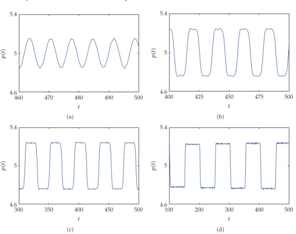
Figures2 and3 describe the phenomena stated in Theorem 2.7, where m 0.65 ∈

3 √2/7,2/3andv 5. It is shown that the time delay plays an important role in the dynamics of the nonlinear model. To be concrete, the longer the time delays used by the chartists in estimating the asset price trend, the more likely the market will exhibit persistent deviation of the asset price from the fundamental value by a limit cycle, and the greater the period of a limit cycle becomes. In fact,τ0 2.885 andc10 −0.856 under these parameters.

Therefore, combining Theorem2.7with the two figures, we know that there exists at least one stable periodic solution ofPwith periodTτ≥2π/ω6.9706 whenτ >2.885. We would like to mention that the graphs in Figure2are prepared by using DDE-BIFTOOL developed by Engelborghs et al.20,21.

3. Proof of the Results in Cases

1 and

2

Case 1. Choosingmas parameter.

When m 1, Pis a scalar ordinary diﬀerential equation and therefore it has no nonconstant periodic solutions. Additionally, the only root of 2.7 isλ −v < 0. These complete the proof of Proposition2.1.

Whenm <1,iηη >0is a root of2.7if and only ifηsatisfies

sinητ η 1−mv, cosητ 1−2m 1−m. 3.1 It follows that 2−cosητη−vsinητ0, m1− 1 2−cosητ. 3.2

(6)

0 τ0 τ1 τ2 τ3 τ4 · · ·τj · · · max p t − min p t a τ0 τ1 τ2 τ3 τ4 · · · τj · · · T τ 2π/ω0 0 b

Figure 2: Hopf bifurcation branches through the centersv, τj,2π/ω0.aon theτ, d-plane, whered

maxpt−minpt;bon theτ, Tτ-plane, whereTτis the period of periodic solution bifurcated at v.

DenoteGηdef 2−cosητη−vsinητ. ThenG0 0, G∞ ∞, and

Gηητsinητ 2−1 vτcosητ. 3.3 Therefore, there exists at least one zeroηkofGηifvτ >1.

Definemkas in2.8, thenmk ∈0,2/3and±iηkis a pair of purely imaginary roots

of2.7withmmk. Letλmbe the root of2.7satisfyingλmk iηk. Substitutingλm

into2.7, it follows that

dλ dm ve−λτ−2v 1−τ1−mve−λτ. 3.4

Thus, we have the transversal condition

Sign Re dλ dm | mmk Sign cosηkτ−2−τv1−mk 1−2 cosηkτ Sign 3τv1−mk2−2τv1−mk−1 1−mk , ⎧ ⎪ ⎪ ⎪ ⎪ ⎪ ⎪ ⎪ ⎨ ⎪ ⎪ ⎪ ⎪ ⎪ ⎪ ⎪ ⎩ 1, mk∈ 0,1 3 2− 1 3 τv , −1, mk∈ 1 3 2− 1 3 τv ,2 3 , 3.5

where cosηkτ 2−1/1−mkis used. Accordingly, a Hopf bifurcation atp∗voccurs when

(7)

4.6 5 5.4 p t 460 470 480 490 500 t a 4.6 5 5.4 p t 400 425 450 475 500 t b 4.6 5 5.4 p t 300 350 400 450 500 t c 4.6 5 5.4 p t 100 200 300 400 500 t d

Figure 3: Stable periodic solution ofP, whereawithτ 2.9> τ0 2.885,bwithτ 10,cwith

τ20, anddwithτ50.

In summary, ifvτ >1, then there exists at least one value ofmdefined by2.8such that all the roots of2.7have negative real parts whenm ∈ m0,1, in addition, a pair of

purely imaginary roots whenmmk. This implies Theorem2.2.

Case 2. Regardingτas a parameter.

First of all, we know that the root of 2.7 with τ 0 satisfies thatλ −mv < 0. Therefore,p∗vis globally asymptotically stable whenτ 0.

Letiωω >0be a root of2.7. Then

sinωτ ω

1−mv >0, cosωτ

1−2m

1−m . 3.6

This leads toω2 _mv2₂₋₃_m_._ω

0 v m2−3mmakes sense whenm∈0,2/3. Define

τjas in2.10; theniω0is a pure imaginary root of2.7withτ τj, j 0,1,2, . . ..

Similarly, letλτ ατ iτbe the root of2.7, satisfying

ατj

0, τj

(8)

Diﬀerentiating both sides of2.7gives dλ dτ −1 eλτ λv1−m − τ λ. 3.8 Therefore, Re dλ dτ −1 | ττj sinω0τj ω0v1−m >0. 3.9

This implies thatατj>0, j 0,1,2,. . ..

Note thatλ0 is not a root of2.7whenm2/3. Therefore, we obtain the following spectral properties of2.7:

iifm∈2/3,1, then all roots of2.7have negative real parts;

iiifm∈ 0,2/3, then there exist a sequence values ofτ defined by2.10such that

2.7has a pair of purely imaginary roots±iω0whenτ τj. Additionally, all roots

of2.7have negative real parts whenτ∈0, τ0, all roots of2.7, except±iω0, have

negative real parts whenτ τ0, and2.7has at least a pair of roots with positive

real parts whenτ > τ0.

These spectral properties immediately lead to the dynamics near the positive equilibriumvdescribed in Theorem2.3.

4. Proof of Theorem

2.4

We use the center manifold and normal form theories presented in Hassard et al. 12 to establish the proof of Theorem2.4. Normalizing the delayτby the time scalingt→t/τand using the change of variablespt ptτ, we transformPinto

dp

dtt 1−mτtanh

pt−pt−1pt−mτpt−vpt, P0 whose characteristic equation atpvis

Δ1z:z−1−2mτv 1−mτve−z0. 4.1 Comparing 4.1 with 2.7, we see z λτ for τ /0. Therefore, we obtain the following Lemma.

Lemma 4.1. Assumem∈0,2/3.

iIfτ τj j 0,1,2, . . ., then4.1has a pair of purely imaginary roots±iω0τj, whereτj

(9)

iiLetzτ γτ iζτbe the root of 4.1, satisfying γτj 0 andζτj ω0τj, 4.2 then γτj τjα τj >0, j 0,1,2, . . . . 4.3

iiiAll roots of4.1have negative real parts whenτ∈0, τ0, all roots of4.1, except±iω0τ0,

have negative real parts whenτ τ0, and4.1has at least a pair of roots with positive real

parts whenτ > τ0.

Without loss of generality, we denote the critical valueτ∗ at whichP0undergoes a

Hopf bifurcation atv. Letτ τ∗ μ, thenμ 0 is the Hopf bifurcation value ofP0. Let p1t pt−vand still denotep1tbypt, so thatP0can be written as

dp dtt v τ∗ μ1−2mpt−1−mpt−1 τ∗ μ1−2mp2t−1−mptpt−1 − 1 3v τ∗ μ1−mp3t−3p2tpt−1 3ptp2t−1−p3t−1 O4. 4.4 Forφ∈C−1,0,R, define Lμ φvτ∗ μ1−2mφ0−1−mφ−1. 4.5

By the Riesz representation theorem, there exists a bounded variation functionηθ, μθ ∈

−1,0such that Lμ φ ₀ −1 dηθ, μφθ, forφ∈C−1,0,R. 4.6

In fact, we can choose

ηθ, μ ⎧ ⎪ ⎪ ⎪ ⎨ ⎪ ⎪ ⎪ ⎩ vτ∗ μ1−2m, θ0, 0, θ∈−1,0, vτ∗ μ1−m, θ−1. 4.7

(10)

Define Aμφθ ⎧ ⎪ ⎪ ⎪ ⎨ ⎪ ⎪ ⎪ ⎩ dφθ dθ , θ∈−1,0, ₀ −1 dηξ, μφξ, θ0, hμ, φτ∗ μ1−2mφ20−1−mφ0φ−1 −1 3v τ∗ μ1−mφ30−3φ20φ−1 3φ0φ2−1−φ3−1 O4. 4.8 Furthermore, define the operatorRμas

Rμφθ ⎧ ⎨ ⎩ 0, θ∈−1,0, hμ, φ, θ0; 4.9

then4.4is equivalent to the following operator equation: ˙ xtA μxt R μxt, 4.10 wherextxt θforθ∈−1,0.

Forψ∈C1₀_,₁_,_R_{, define an operator}

A∗ψs ⎧ ⎪ ⎪ ⎪ ⎨ ⎪ ⎪ ⎪ ⎩ −dψs ds , s∈0,1, ₀ −1 ψ−ξdηξ,0, s0 4.11

and a bilinear form ψs, φθψ0φ0− 0 −1 θ ξ0 ψξ−θdηθφξdξ, 4.12

whereηθ ηθ,0, thenA0andA∗are adjoint operators.

From the preceding discussions, we know that±iω0τ∗ are eigenvalues ofA0and

therefore they are also eigenvalues ofA∗. It is not diﬃcult to verify that the vectorsqθ eiω0τ∗θ_θ _∈ ₋₁_,₀ _and _q∗_s _leiω0τ∗s_s _∈ ₀_,₁ _{are the eigenvectors of} _A₀ _and _A∗

corresponding to the eigenvalues iω0τ∗and−iω0τ∗, respectively, where

(11)

Following the algorithms stated in Hassard et al.12, we obtain the coeﬃcients which will be used in determining the important quantities:

g20 2lτ∗ 1−2m−1−me−iω0τ∗, g11 lτ∗ 21−2m−1−meiω0τ∗ e−iω0τ∗, g02 2lτ∗ 1−2m−1−meiω0τ∗, g21 2lτ∗1−2m2W110 W200 −lτ∗1−m2W11−1 W20−1 W200eiω0τ∗ 2W110e−iω0τ∗

−2lτ∗v1−m3−3e−iω0τ∗−eiω0τ∗ _e−2iω0τ∗_,

4.14 where forθ∈−1,0, W20θ ig20 ω0τ∗ qθ ig02 3ω0τ∗ qθ E1e2iω0τ ∗_θ , W11θ − ig11 ω0τ∗ qθ ig11 ω0τ∗ qθ E2, E1 21−2m−1−me−iω0τ∗ 2iω0−v1−2m−1−me−2iω0τ∗ , E2 21−2m−1−meiω0τ∗ _e−iω0τ∗ mv . 4.15

Consequently,g21can be expressed explicitly.

Thus, we can compute the following values:

c10 i 2ω0τ∗ g11g20−2g112− g022 3 g21 2 , μ2− Rec10 Reλτ∗, β22 Rec10, T2− Imc10 μ2Imλτ∗ ω0τ∗ , 4.16

which determine the properties of bifurcating periodic solutions at the critical valueτ∗. More specifically,μ2 determines the directions of the Hopf bifurcation: if μ2 > 0μ2 < 0, then

the bifurcating periodic solutions exist for τ > τ∗ τ < τ∗;β2 determines the stability of

(12)

stable unstableif β2 < 0 β2 > 0;T2 determines the period of the bifurcating periodic

solutions: the period increasesdecreasesifT2>0 T2<0. Thus Theorem2.4follows.

In particular, whenτ τ0m. It is well known that the normal form of the restriction ofP0withττ0on the center manifold is given by

˙

zt iω0τ0z c10z2z · · ·. 4.17

By Liapunov’s second method, the zero solution of4.17is stableunstableif Rec10 <

0>0, and so isv.

5. Proof of Theorem

2.7

Assumem ∈ 0,2/3. It is known thatP undergoes a local Hopf bifurcation at p∗ v

whenτ τjj 0,1, . . .. Now we show that each bifurcation branch can be continued with

respect to the parameterτunder the conditions in Theorem2.7. We introduce the following notations:

XC−τ,0,R,

Σ Cly, τ, T:y is a T−periodic solution of P⊂X×R ×R , Ny, τ, T :y0 orv.

5.1

Let Cv, τj,2π/ω0 denote the connected component of v, τj,2π/ω0 in Σ, and

Proj_τv, τj,2π/ω0its projection onτ component, whereω0 v m2−3mand thus±iω0

is a pair of purely imaginary roots of 2.7 with τ τj. By Theorem 2.3, we know that

Cv, τj,2π/ω0is nonempty.

Lemma 5.1. All bifurcating periodic solutions of Pfrom Hopf bifurcation atvare positive ifτ ∈

Proj_τv, τj,2π/ω0.

Proof. For each τ ∈ Proj_τv, τj,2π/ω0, denote by Xt, τ the corresponding nontrivial

periodic solution, with its minimum value inf_t∈_R Xt, τ. From the fact that the periodic solutions bifurcated from the positive equilibrium are continuous with respect to τ and limτ→τjXt, τ v uniformly in t ∈ R, we have that inft∈RXt, τ is continuous with respect to τ, and the bifurcating periodic solutions are positive when τ varies in a small neighborhood of τj. To prove the positivity, it is equivalent to prove inft∈RXt, τ > 0

when τ ∈ Proj_τv, τj,2π/ω0. Otherwise, there exists a τ∗ ∈ Proj_τv, τj,2π/ω0such that

inf_t∈_RXt, τ∗ 0. Without loss of generality, we assume thatτ∗ > τj and inft∈RXt, τ > 0 whenτ ∈τj, τ∗. By the proof of positivity of solution, we obtainXt, τ∗≡ 0. This implies

that0, τ∗,2π/ωis a center ofPfor someω >0. This contradiction completes the proof.

Lemma 5.2. Ifm∈3 √2/7,2/3, thenPhas no positive periodic solution of period 4τ.

Proof. Suppose thatytis a positive periodic solution toPof period 4τ. Set

ujt y

(13)

Thenut u1t, u2t, u3t, u4tis a periodic solution to the following system of ordinary diﬀerential equations: ˙ u1t 1−mtanhu1−u2u1−mu1−vu1, ˙ u2t 1−mtanhu2−u3u2−mu2−vu2, ˙ u3t 1−mtanhu3−u4u3−mu3−vu3, ˙ u4t 1−mtanhu4−u1u4−mu4−vu4, 5.3

where·denotes d/dt. Let

G u∈R:uj∈ 0,1−m m v , j1,2,3,4 . 5.4

ForP, the ultimate uniform boundedness of solutions implies that the periodic solutions of

Pbelong to the regionG. To rule out the 4τ-periodic solution toP, it suﬃces to prove the nonexistence of nonconstant periodic solutions of5.3in the regionG. To do the latter, we use a general Bendixson’s criterion in higher-dimensions developed by Li and Muldowney

19. More specifically, we shall apply19, Corollary 3.5. The Jacobian matrixJ Ju of

5.3, foru∈R4_{, is} Ju ⎛ ⎜ ⎜ ⎜ ⎜ ⎜ ⎝ A1 B1 0 0 0 A2 B2 0 0 0 A3 B3 B4 0 0 A4 ⎞ ⎟ ⎟ ⎟ ⎟ ⎟ ⎠. 5.5 Fori1,2,3,4, Ai 1−m uitanh1ui−ui 1 tanhui−ui 1 −2mui mv, Bi−1−muitanh1ui−ui 1<0, 5.6

withu5u1. The second additive compound matrixJ2uofJuis

J2u ⎛ ⎜ ⎜ ⎜ ⎜ ⎜ ⎜ ⎜ ⎜ ⎜ ⎜ ⎜ ⎝ A1 A2 B2 0 0 0 0 0 A1 A3 B3 −B1 0 0 0 0 A1 A4 0 B1 0 0 0 0 A2 A3 B3 0 −B4 0 0 0 A2 A4 B2 0 −B4 0 0 0 A3 A4 ⎞ ⎟ ⎟ ⎟ ⎟ ⎟ ⎟ ⎟ ⎟ ⎟ ⎟ ⎟ ⎠ . 5.7

(14)

Choose a vector norm inR6_as |x1, x2, x3, x4, x5, x6| max '√ 2|x1|,|x2|, √ 2|x3|, √ 2|x4|,|x5|, √ 2|x6| ( . 5.8

Then with respect to this norm, the Lozinskii measureμJ2_u_{of the matrix}_J2_u_is_see

22 μJ2umax Ai Aj− √ 2Bi, Ap Aq− √ 2 2 Bp Bq , 5.9

with i, j ∈ {1,4,2,1,3,2,4,3}, and p, q ∈ {1,3,2,4}. By 19, Corollary 3.5, system 5.3 has no periodic orbits in the regionG ifμJ2u < 0 for all u ∈ G. In fact, whenm∈3 √2/7,2/3, one can acquire the inequality as below,

μJ2_u_<₁₋_m _mv ) 2 21−3m √ 21−m m * <0. 5.10

This completes the proof.

Lemma 5.3. EquationPhas no nonconstant periodic solution of periodτ.

Proof. EquationPhas no nonconstant periodic solution of periodτis equivalent to the fact

thatP withτ 0 has no nonconstant periodic solution. It is straightforward that a first order autonomous ODE has no nonconstant periodic solutions.Pwithτ0 is a first-order autonomous ODE, which proves the lemma.

Proof of Theorem2.7. First note that for anyτj, the stationary pointsv, τj,2π/ω0ofPare

nonsingular and isolated centerssee Wu13under the assumptionm∈0,2/3; then the hypothesisH2in13 is satisfied. By3.9, there exist > 0, δ > 0 and a smooth curve

λ:τj−δ, τj δ → C, such that

Δλτ Δ_v,τ,Tλτ 0, |λτ−iω0|< , 5.11

for allτ∈τj−δ, τj δ, whereΔis defined as2.7, and

λτj

iω0,

dReλτ

dτ |ττj>0. 5.12

Denotepj 2π/ω0and let Ω

0, q: 0< u < ,q−pj<

(15)

Clearly, if|τ−τj| ≤δandu, q∈Ωsuch thatΔv,τ,Tu 2πi/q 0, thenτ τj, u0, and qpj. Moreover, putting H± v, τj,2π ω0 u, q Δv,τj±δ,T u i2π q , 5.14

we have the crossing number

γ1 v, τj, 2π ω0 deg_B H− v, τj, 2π ω0 ,Ω −deg_B H v, τj, 2π ω0 ,Ω −1. 5.15 By the local Hopf bifurcation theorem for FDE 10, we conclude that the connected componentCv, τj,2π/ω0throughv, τj,2π/ω0inΣis nonempty. Meanwhile, we have

+ y,τ,T ∈Cv,τj,2π/ω0 γ1 y, τ, T<0 5.16

and thusCv, τj,2π/ω0is unbounded by the global Hopf bifurcation theorem given by Wu

13.

Again, the property of ultimate uniform boundedness implies that the projection of Cv, τj,2π/ω0 onto the y-space is bounded. Meanwhile, P with τ 0 has no

nonconstant periodic solutions since it is a first-order autonomous ordinary diﬀerential equation. Therefore, Proj_τv, τj,2π/ω0is bounded below.

By the definition ofτjgiven in2.10, we know that, whenm∈0,2/3,

2π < τjω0<2

j 1π, j ≥1, 5.17 which implies that

τj

j 1 < 2π ω0

< τj. 5.18

By Lemma5.3, we have τ/j 1 < T < τ ifx, τ, T ∈ Cv, τj,2π/ω0forj ≥ 1. Because

Cv, τj,2π/ω0 is unbounded, Projτv, τj,2π/ω0 must be unbounded. Consequently,

Proj_τv, τj,2π/ω0includeτj,∞forj≥1. The former part of the theorem follows.

Moreover, ifm∈3 √2/7,2/3, then

π

2 < τ0ω0< π, 5.19 where3.6is used. This implies that

2τ0< 2π

ω0

(16)

Thus, we have by Lemma 5.2 that 2τ < T < 4τ if x, τ, T ∈ Cv, τ0,2π/ω0. Similarly,

this shows that in order for Cv, τ0,2π/ω0to be unbounded, Proj_τv, τ0,2π/ω0must be

unbounded. This implies that Proj_τv, τ0,2π/ω0includesτ0,∞.

In addition, the first global Hopf branch contains periodic solutions with period between 2τand 4τ, which are the slowly oscillating periodic solutions. Thejth branches, for

j ≥ 1, since the periods are less thanτ, contain fast-oscillating periodic solutions. Therefore,

Phas at least two periodic solutions forτ > τ0providedm∈3 2/7,2/3. The proof

of Theorem2.7is complete.

Acknowledgments

This research is supported by the NNSFno. 10771045of China, the Program of Excellent Team in HIT and the Natural Science Foundation of Heilongjiang Province,A200806. The authors are grateful to Professor Xuezhong He and the anonymous referees for their helpful comments and valuable suggestions.

References

1 C. Chiarella, R. Dieci, and L. Gardini, “Speculative behaviour and complex asset price dynamics: a global analysis,” Journal of Economic Behavior and Organization, vol. 49, no. 2, pp. 173–197, 2002.

2 C. Chiarella, R. Dieci, and X. He, “Heterogeneity, market mechanisms and asset price dynamics,” in

Handbook of Financial Markets: Dynamics and Evolution, chapter 5, pp. 277–344, 2009.

3 C. Chiarella and X.-Z. He, “Heterogeneous beliefs, risk, and learning in a simple asset-pricing model with a market maker,” Macroeconomic Dynamics, vol. 7, no. 4, pp. 503–536, 2003.

4 G. Dibeh, “Speculative dynamics in a time-delay model of asset prices,” Physica A, vol. 355, no. 1, pp. 199–208, 2005.

5 X.-Z. He, K. Li, J. Wei, and M. Zheng, “Market stability switches in a continuous-time financial market with heterogeneous beliefs,” Economic Modelling, vol. 26, no. 6, pp. 1432–1442, 2009.

6 C. H. Hommes, “Financial markets as nonlinear adaptive evolutionary systems,” Quantitative Finance, vol. 1, no. 1, pp. 149–167, 2001.

7 C. Hommes, “heterogeneous agent models in economics and finance,” in Handbook of Computational

Economics, vol. 2, chapter 23, pp. 1109–1186, 2006.

8 T. Lux, “The socio-economic dynamics of speculative markets: interacting agents, chaos, and the fat tails of return distributions,” Journal of Economic Behavior and Organization, vol. 33, no. 2, pp. 143–165, 1998.

9 R. Sethi, “Endogenous regime switching in speculative markets,” Structural Change and Economic

Dynamics, vol. 7, no. 1, pp. 99–118, 1996.

10 J. K. Hale and S. M. V. Lunel, Introduction to Functional-Diﬀerential Equations, vol. 99 of Applied Mathematical Sciences, Springer, New York, NY, USA, 1993.

11 J. Carr, Applications of Centre Manifold Theory, vol. 35 of Applied Mathematical Sciences, Springer, New York, NY, USA, 1981.

12 B. D. Hassard, N. D. Kazarinoﬀ, and Y. H. Wan, Theory and Applications of Hopf Bifurcation, vol. 41 of

London Mathematical Society Lecture Note Series, Cambridge University Press, Cambridge, UK, 1981.

13 J. H. Wu, “Global continua of periodic solutions to some diﬀerence-diﬀerential equations of neutral type,” The Tohoku Mathematical Journal, vol. 45, no. 1, pp. 67–88, 1993.

14 J. Wei, “Bifurcation analysis in a scalar delay diﬀerential equation,” Nonlinearity, vol. 20, no. 11, pp. 2483–2498, 2007.

15 J. Wei and D. Fan, “Hopf bifurcation analysis in a Mackey-Glass system,” International Journal of

Bifurcation and Chaos, vol. 17, no. 6, pp. 2149–2157, 2007.

16 J. Wei and M. Y. Li, “Hopf bifurcation analysis in a delayed Nicholson blowflies equation,” Nonlinear

Analysis: Theory, Methods & Applications, vol. 60, no. 7, pp. 1351–1367, 2005.

17 J. Wei and C. Yu, “Hopf bifurcation analysis in a model of oscillatory gene expression with delay,”

(17)

18 J. H. Wu, “Symmetric functional-diﬀerential equations and neural networks with memory,”

Transactions of the American Mathematical Society, vol. 350, no. 12, pp. 4799–4838, 1998.

19 Y. Li and J. S. Muldowney, “On Bendixson’s criterion,” Journal of Diﬀerential Equations, vol. 106, no. 1,

pp. 27–39, 1993.

20 K. Engelborghs, T. Luzyanina, and D. Roose, “Numerical bifurcation analysis of delay diﬀerential equations using DDE-BIFTOOL,” Association for Computing Machinery, vol. 28, no. 1, pp. 1–21, 2002.

21 K. Engelborghs, T. Luzyanina, and G. Samaey, “DDE-BIFTOOL v. 2.00: a matlab package for bifurcation analysis of delay diﬀerential equations,” Technical Report TW-330, Department of Computer Science, K. U. Leuven, Leuven, Belgium, 2001.

22 W. A. Coppel, Stability and Asymptotic Behavior of Diﬀerential Equations, D. C. Heath, Boston, Mass,

(18)

Submit your manuscripts at

http://www.hindawi.com

Hindawi Publishing Corporation

http://www.hindawi.com Volume 2014

Mathematics

Journal of

Mathematical Problems in Engineering

Hindawi Publishing Corporation http://www.hindawi.com

Differential Equations

International Journal of

Volume 2014 Hindawi Publishing Corporation

http://www.hindawi.com Volume 2014 Hindawi Publishing Corporationhttp://www.hindawi.com Volume 2014

Mathematical PhysicsAdvances in

Complex Analysis

Journal of

Optimization

Journal of Hindawi Publishing Corporation

Combinatorics

Journal of

Function Spaces

Abstract and Applied Analysis Hindawi Publishing Corporation

http://www.hindawi.com Volume 2014 International Journal of Mathematics and Mathematical Sciences

Hindawi Publishing Corporation http://www.hindawi.com Volume 2014

The Scientific

World Journal

Discrete Dynamics in Nature and Society

Discrete Mathematics

Journal of

http://www.hindawi.com Volume 2014 Hindawi Publishing Corporationhttp://www.hindawi.com Volume 2014

Research Article Global Hopf Bifurcation Analysis for a Time-Delayed Model of Asset Prices