Estimating Smooth Structural Change in Cointegration Models
1 Peter C. B. Phillips2, Degui Li3 and Jiti Gao4Abstract
This paper studies nonlinear cointegration models in which the structural coefficients may evolve smoothly over time, and considers time-varying coefficient functions estimated by nonparametric kernel methods. It is shown that the usual asymptotic methods of kernel estimation completely break down in this setting when the functional coefficients are multivariate. The reason for this breakdown is a kernel-induced degeneracy in the weighted signal matrix associated with the non-stationary regressors, a new phenomenon in the kernel regression literature. Some new techniques are developed to address the degeneracy and resolve the asymptotics, using a path-dependent local coordinate transformation to re-orient coordinates and accommodate the degeneracy. The resulting asymptotic theory is fundamentally different from the existing kernel literature, giving two different limit distributions with different convergence rates in the different directions of the (functional) pa-rameter space. Both rates are faster than the usual root-nhrate for nonlinear models with smoothly changing coefficients and local stationarity. In addition, local linear methods are used to reduce asymptotic bias and a fully modified kernel regression method is proposed to deal with the general endogenous nonstationary regressor case, which facilitates inference on the time varying functions. The finite sample properties of the methods and limit theory are explored in simulations. A brief empirical application to macroeconomic data shows that a linear cointegrating regression is rejected but finds support for alternative polynomial approximations for the time-varying coefficients in the regression.
Key words and phrases: Cointegration; Endogeneity; Kernel degeneracy; Nonparametric regression; Super-consistency; Time varying coefficients.
JEL classification: C13, C14, C32.
Abbreviated title: Smooth Change in Cointegration Models
1The authors thank the Co–Editor, Oliver Linton, an Associate Editor and three anonymous referees for
comments and suggestions on the previous version of the paper. The work was commenced during November 2012 while the first author visited Monash University. Phillips thanks the Department of Econometrics at Monash for its hospitality during this visit and acknowledges support from a Kelly Felllowship and the NSF under Grant Numbers: SES 0956687 and SES 1258258. Gao acknowledges support from the ARC under Grant Numbers: DP1314229 and DP150101012.
2Yale University, University of Auckland, Southampton University, and Singapore Management University 3University of York
1
Introduction
Cointegration models are now one of the most commonly used frameworks for applied research in econometrics, capturing long term relationships among trending macroeconomic time series and present value links between asset prices and fundamentals in finance. These models conveniently combine stochastic trends in individual series with linkages between series that eliminate trending behavior and reflect latent regularities in the data. In spite of their importance and extensive research on their properties (e.g. Park and Phillips, 1988; Johansen, 1988; Phillips, 1991; and Saikkonen, 1995; among many others) linear cointegration models are often rejected by the data even when there is clear co-movement in the series.
Various nonlinear parametric cointegrating models have been suggested to overcome such de-ficiencies. These models have been the subject of an increasing amount of econometric research following the development of methods for handling nonlinear nonstationary process asymptotics (Park and Phillips, 1999, 2001). However, parameter instability and functional form misspecifi-cation may limit the performance of such nonlinear parametric cointegration models in empirical applications (Hong and Phillips, 2010; Kasparis and Phillips, 2012; Kaspariset al, 2013). Most re-cently, therefore, attention has been given to flexible nonparametric and semiparametric approaches that can cope with the unknown functional form of responses in a nonstationary time series setting (Karlsen et al, 2007; Wang and Phillips, 2009a, 2009b, 2015; Gao and Phillips, 2013a). A futher extension of the linear framework allows cointegrating relationships to evolve smoothly over time using time-varying cointegrating coefficients (e.g. Park and Hahn, 1999; Juhl and Xiao, 2005; Cai
et al, 2009; Xiao, 2009). This framework seems particularly well suited to empirical applications where there may be structural evolution in a relationship over time, thereby tackling one of the main limitations of fixed coefficient linear and nonlinear formulations. It is this framework that is the subject of the present investigation.
More specifically, we consider the following cointegration model with time-varying coefficient functions
yt=x′tf
(
t/n)+ut=x′tft+ut, t= 1,· · ·, n, (1.1)
where f(·) is a d-dimensional function of time (measured as a fraction of the sample size), xt is an I(1) vector, and ut is a scalar process. The function f(t/n) is sometimes called a fixed design and, in the present context, may be regarded as a weak trend function so that the model (1.1) cap-tures potential drifts in the cointegrating linkage relationship between yt and xt over time. Such a modeling structure is especially useful for time series data over long horizons where economic mechanisms are likely to evolve and be subjected to changing institutional or regulatory conditions. For example, firms may change production processes in response to technological innovation and consumers may change consumption and savings behavior in response to new products and new banking regulations. These changes may be captured by temporal evolution in the coefficients through the functional dependence f(t/n) in the model (1.1). Thus model (1.1) allows the long term relationships among the trending time series to evolve smoothly over time, which provides
a more flexible framework than the parametric linear and nonlinear cointegration models. Some recent papers including Caiet al (2009), Xiao (2009), Gao and Phillips (2013b) and Liet al (2016) studied a nonlinear cointegrating model with functional coefficients and its generalised version, where the index variable in the functional coefficients is random, and developed the associated asymptotic theory. However, it is often difficult to select an appropriate random covariate as the index variable in practical applications and the requisite data may not be available. Such consid-erations partly motivate the use of a generic time-varying function to explore potential evolution in the cointegrating relationship betweenyt andxtin model (1.1). Nonparametric inference about
time-varying parameters has received attention for modeling stationary or locally stationary time series data - see, for instance, Robinson (1989), Cai (2007), Liet al (2011), Chen and Hong (2012), and Zhang and Wu (2012). However, there is little literature on this topic for integrated or coin-tegrated time series. One exception is Park and Hahn (1999), who considered the time-varying parameter model (1.1) and used sieve methods to transform the nonlinear cointegrating equation to a linear approximation with a sieve basis of possibly diverging dimension. Their asymptotic theory can be seen as an extension of the work by Park and Phillips (1988).
The present paper seeks to uncover evolution in the modeling framework for nonstationary time series over a long time horizon by using nonparametric kernel regression methods to estimate
f(·), and our asymptotic theory is fundamentally different from that in the paper by Park and Hahn (1999). Our treatment shows that estimation of this model by conventional kernel methods encounters a degeneracy problem in the weighted signal matrix (the denominator of the kernel estimator (2.1)), which introduces a major new challenge in developing the limit theory. In fact, kernel degeneracy of this type can arise in many contexts where multivariate time-varying functions are associated with nonstationary regressors. The present literature appears to have overlooked the problem and existing mathematical tools fail to address it. The reason for degeneracy in the limiting weighted signal matrix is that kernel regression concentrates attention on a particular (time) coordinate, thereby fixing attention on a particular coordinate of f and the associated limit process of the regressor. In the multivariate case this focus on a single time coordinate produces a limiting signal matrix of deficient rank one whose zero eigenspace depends on the value of the limit process at that time coordinate. In other words, kernel degeneracy in the signal matrix is random and trajectory dependent.
This paper introduces a novel method to accommodate the degeneracy in kernel limit theory. The method transforms coordinates to separate the directions of degeneracy and non-degeneracy and proceeds to establish the kernel limit theory in each of these directions. The asymptotics are fundamentally different from those in the existing literature. As intimated, the transformation is path dependent and local to the coordinate of concentration. Two different convergence rates are obtained for different directions (or combinations) of the multivariate nonparametric estimators, and both of the two rates are faster than the usual (√nh) rate of stationary kernel asymptotics. Thus, two types of super-consistency exist for the nonparametric kernel estimation of time-varying
coefficient functions, which we refer to as type I and type II super-consistency. The higher rate of convergence (n√h) lies in the direction of the nonstationary regressor vector at the local coordinate point and exceeds the usual√nh-rate by√n(type I super-consistency). The lower rate (nh) lies in the degenerate direction but is still super-consistent (type II super-consistency) for nonparametric estimators and exceeds the usual √nh-rate by √nh.
The above results are all obtained for the Nadaraya-Watson local level time varying coefficient regression in a cointegrating model. Similar results are shown to apply for local linear time-varying regression which assists in reducing asymptotic bias. The general case of endogenous cointegrating regression is also included in our framework and a fully modified (FM; Phillips and Hansen, 1990) kernel method is proposed to address the endogeneity of the nonstationary regressors. In the use of this method it is interesting to discover that the kernel estimators need to be modified through bias correction only in the degenerate direction as the limit distribution of the estimators is not affected by the possible endogeneity in the direction of the nonstationary regressor vector at the local coordinate point. The limit theory for FM kernel regression also requires new asymptotic results on the consistent estimation of long run covariance matrices, which in turn involve uniform consistency arguments because of the presence of nonparametric regression residuals in these es-timates. Importantly, inference about the time varying coefficient functions is unaffected by the degeneracy once the FM correction is made.
The remainder of the paper is organized as follows. Estimation methodology, some technical-ities, and assumptions are given in Section 2. This section also introduces the kernel degeneracy problem, explains the phenomenon, and provides intuition for its resolution. Asymptotic properties of the nonparametric kernel estimator are developed in Section 3 with accompanying discussion. A kernel weighted FM regression method is proposed with attendant limit theory in Section 4. Section 5 reports simulation findings on the finite sample properties of the methods and limit the-ory, and gives a practical application of these time-varying kernel regression methods to empirical relationships involving consumption, disposable income, investment and real interest rates. Section 6 concludes the paper. Proofs of the main theoretical results in the paper are given in Appendix A. Some supplementary technical materials and discussions on model specification testing are provided in an online supplement (Phillips, Li and Gao, 2016).
2
Kernel estimation degeneracy
Set τ =⌊nδ⌋where the floor function ⌊·⌋ denotes integer part and δ∈[0,1] is the sample fraction corresponding to observationt. The functional response in (1.1) allows the regression coefficient to vary over time and kernel regression provides a convenient mechanism for fitting the function locally at a particular (time) coordinate, say τ = ⌊nδ⌋. At this coordinate the coefficient is the vector
f(⌊nδ⌋/n) ∼ f(δ) and the model response behaves locally around τ as xτ′f(τ /n) ∼ x′⌊nδ⌋f(δ).
functional dependence x′⌊nδ⌋f(δ).
Under certain smoothness conditions onf and for some fixedδ0 ∈(0,1) we have
f(t/n) =f(δ0) +O ( t n−δ0 ) ≈f(δ0)
when nt is in a small neighborhood ofδ0. The Nadaraya-Watson type local level regression estimator of f(δ0) has the usual form given by
b fn(δ0) = [ n ∑ t=1 xtx′tKth(δ0) ]+[∑n t=1 xtytKth(δ0) ] , Kth(δ0) = 1 hK ( t−nδ0 nh ) , (2.1)
where A+ denotes the generalized inverse of A, K(·) is some kernel function, and h is the band-width. Extensions to allow for multiple (distinct) coordinates {δi :i= 1,· · ·, I} of concentration are straightforward.
The random matrix in the denominator of the local level regression estimation (2.1) is called the signal matrix throughout this paper as it carries the sample signal information in the re-gressors about the coefficient function f locally in the neighborhood of the fixed point δ0. The weightsKth(δ0) in the estimation (2.1) ensure that the primary contributions to the signal matrix
∑n
t=1xtx′tKth(δ0) come from observations in the immediate temporal neighborhood of τ . In
gen-eral, we can expect there to be sufficient variation inxtwithin this temporal neighborhood for the signal matrix ∑nt=1xtx′tKth(δ0) to be positive definite in finite samples, i.e. for fixednand h >0.
In the case of stationary and independent generating mechanisms forxt,the variation inxtis also sufficient to ensure a positive definite limit as n→ ∞ and h→0 because the second moment ma-trix E(xtx′t) may be assumed to be positive definite. However, in the nonstationary case wherext
converges weakly to a continuous stochastic process upon standardization, localizing the regression around a fixed point such as δ0 reduces effective variability in the regressor when n→ ∞because of continuity in the limit process and therefore leads to rank degeneracy in the limit of the signal matrix after standardization. The generalized inverse is employed in (2.1) for this reason. This limiting degeneracy in the weighted signal matrix challenges the usual approach to developing ker-nel asymptotics. As is apparent from the above explanation, limiting degeneracy of this type may be anticipated whenever kernel regression is conducted to fit multivariate time-varying functions that are associated with nonstationary regressors.
To develop the limit theory we start with some regularity conditions to characterize the non-stationary time series xt and the (scalar) stationary error process ut. We assumext is a unit root process with generating mechanismxt=xt−1+vt,initial valuex0=OP(1), and innovations jointly
determined with the equation errors ut according to the linear process
wt= (vt′, ut)′ = Φ(L)εt=
∞
∑
j=0
Φjεt−j, (2.2)
where Φ(L) =∑∞j=0ΦjLj, Φj is a sequence of (d+ 1)×(d+ 1) matrices,L is the lag operator, and
(d+ 1). Such a generation onutand vt has been commonly used in the literature such as Phillips (1995). Partition Φj as Φj = [Φj,1, Φj,2]′ so that vt= ∞ ∑ j=0 Φ′j,1εt−j, and ut= ∞ ∑ j=0 Φ′j,2εt−j.
We use ∥ · ∥to denote the Euclidean norm of a vector or the Frobenius norm of a matrix.
Assumption 1. Let εt be iid (d+ 1)-dimensional random vectors with E[εt] = 0, Λ0 ≡E[εtε′t]>
0, and E[∥εt∥4+γ0] < ∞ for γ0 > 0. The linear process coefficient matrices in (2.2) satisfy
∑∞
j=0j∥Φj∥<∞.
By functional limit theory for a standardized linear process (Phillips and Solo, 1992) and noting that
n−1/2
⌊∑nr⌋ s=1
εs⇒Bε,r(Λ0)
withBε,r(Λ0) being (d+ 1)-dimensional Brownian motion (BM) with variance matrix Λ0,, we have
fort=⌊nr⌋ and 0< r≤1, xt √ n = 1 √ n t ∑ s=1 vs+ √1 nx0 = 1 √ n ⌊∑nr⌋ s=1 vs+oP(1)⇒Bd,r(Ωv), (2.3) n−1/2 ⌊∑nr⌋ s=1 ws⇒Bd+1,r(Ω), n−1/2 ⌊nr⌋ ∑ s=1 us⇒Br(Ωu), (2.4)
where Bd+1,r(Ω) = [Bd,r(Ωv)′, Br(Ωu)]′ is (d+ 1)-dimensional BM with variance matrix Ω, and
Ω = Φ(1)′Λ0Φ(1) = Φ1(1) ′Λ 0Φ1(1) Φ1(1)′Λ0Φ2(1) Φ2(1)′Λ0Φ1(1) Φ2(1)′Λ0Φ2(1) ≡ Ωv Ωvu Ωuv Ωu , (2.5) with Φ(1) = ∑∞j=1Φj,Φ1(1) = ∑∞ j=1Φj,1, and Φ2(1) = ∑∞
j=1Φj,2. Here Ω is the partitioned long
run variance matrix ofwt= (v′t, ut)′.The limit theory also involves the partitioned components of the one-sided long run variance matrix
∆ww≡ ∆vv ∆vu ∆uv ∆uu = ∞ ∑ j=0 E(w−jw′0).
It is convenient to impose a smoothness condition on the functional coefficient f(·) and some commonly-used conditions on the kernel function and bandwidth. Define µj =∫−11ujK(u)duand
νj =
∫1
−1u
jK2(u)du.
Assumption 2. f(·) is continuous with|f(δ0+z)−f(δ0)|=O(|z|γ1) asz→0for some 12 < γ1 ≤
Assumption 3. (i) The kernel function K(·) is continuous, positive, symmetric and has compact
support [−1,1]with µ0 = 1.
(ii) The bandwidth h satisfies h→0 andnh→ ∞.
In the linear cointegration model with constant coefficients
yt=x′tβ+ut, xt=xt−1+vt, t= 1,· · · , n, (2.6)
where vt and ut are generated by (2.2) and satisfy Assumption 1, least squares estimation of β
gives bβn= (∑nt=1xtx′t)−1(∑nt=1xtyt). Standard limit theory and super-consistency results forβbn
involve the following behavior of the signal matrix 1 n2 n ∑ t=1 xtx′t= 1 n n ∑ t=1 xt √ n x′t √ n ⇒ ∫ 1 0 Bd,r(Ωv)Bd,r(Ωv)′dr, (2.7)
where the limit matrix is positive definite (Phillips and Hansen, 1990). By naive analogy to (2.7) it might be anticipated that the weighted signal matrix appearing in the denominator of the kernel estimator fnb(δ0) would have similar properties. However, some simple derivations show this not to be the case, as we now demonstrate.
Take a neighborhoodNnδ0(h) =
[
⌊(δ0−h)n⌋,⌊(δ0+h)n⌋
]
of⌊δ0n⌋and letδn=⌊(δ0−h)n⌋. The
following representation of the weighted signal matrix is convenient in obtaining the limit behavior
n ∑ t=1 xtx′tKth(δ0) = n ∑ t=1 xδnx′δnKth(δ0) + n ∑ t=1 (xt−xδn)x′δnKth(δ0) + n ∑ t=1 xδn(xt−xδn) ′K th(δ0) + n ∑ t=1 (xt−xδn) (xt−xδn) ′K th(δ0)
≡Un1+Un2+Un3+Un4. (2.8)
Using the BN decomposition as in Phillips and Solo (1992), we have
xt−xt−1 =vt=vt+ (evt−1−evt), where vt= (∑∞ j=0Φ′j,1 ) εt= Φ1(1)′εt, andvet= ∑∞ j=0Φe′j,1εt−j withΦej,1= ∑∞ k=j+1Φk,1. Then xδn = δn ∑ t=1 vt+x0= δn ∑ t=1 vt+ev0−evδn+x0. (2.9)
By virtue of Assumption 1, we have 1 δn (δ n ∑ t=1 vt ) (δ n ∑ t=1 vt )′ = Φ1(1)′ [ 1 δn (δ n ∑ t=1 εt ) (δ n ∑ t=1 ε′t )] Φ1(1) ⇒Φ1(1)′Wd+1(Λ0)Φ1(1), (2.10)
where Wd+1(Λ0) = Bε,δ0(Λ0)Bε,δ0(Λ0)′ is a Wishart variate with 1 degree of freedom and mean
matrix Λ0. Note that the summability condition
∑∞
j=0j∥Φj∥ < ∞ ensures
∑∞
j=0∥Φej∥ < ∞
(Phillips and Solo, 1992), so that
(ev0−evδn+x0) (ev0−evδn+x0)
and then ( δn ∑ t=1 vt ) (ev0−evδn+x0) ′ =O P( √ n) =oP(n). (2.12)
On the other hand, by Assumption 3, we have n1 ∑nt=1Kth(δ0) → µ0 = 1 for 0 < δ0 < 1 which, together with (2.9)–(2.12), implies that
1 n2Un1 = ( xδnx′δn n ) ( 1 n n ∑ t=1 Kth(δ0) ) ⇒ δ0Φ′1(1)Wd+1(Λ0)Φ1(1). (2.13)
Next observe that fort∈Nnδ0(h) which is a set of integers inNnδ0(h), we havext−xδn = ∑t s=δn+1vs and then sup t∈Nnδ0(h) xt−xδn √ 2⌊nh⌋ =t∈Nsup nδ0(h) ∑t s=δn+1vs √ 2⌊nh⌋ ⇒0<r<1sup ∥ Bd,r(Ωv)∥, (2.14)
where Bd,r(Ωv) is the Brownian motion with covariance matrix Ωv defined as in (2.3). Hence, for h→0 as n→ ∞ we have sup t∈Nnδ0(h) xt√−xδn nh =OP(1).
For Un2, by Assumption 3 and the fact thatK(·) has compact support, we find that
∥Un2∥ ≤ ∥xδn∥ [(δ0∑+h)n] t=[(δ0−h)n]+1 Kth(δ0)∥xt−xδn∥ = OP (√ n)×OP ( n)×OP (√ nh) = OP(n2h1/2)=oP(n2). (2.15) Similarly, ∥Un3∥=OP ( n2h1/2)=oP ( n2), (2.16) and ∥Un4∥=OP(n2h)=oP (n2). (2.17) In view of (2.8) and (2.13)–(2.17), we deduce that
1 n2 n ∑ t=1 xtx′tKth(δ0)⇒δ0Φ′1(1)Wd+1(Λ0)Φ1(1), (2.18)
which is the limiting signal matrix analogue of (2.7) in the case of nonparametric kernel-weighted least squares. On inspection, thed×dlimit matrix Φ′1(1)Wd+1(Λ0)Φ1(1) in (2.18) is singular with
rank one whend >1. The weighted signal matrix n12
∑n
t=1xtx′tKth(δ0) is therefore asymptotically
singular whenever the dimension of the regressor xt exceeds unity.
The intuition for this limiting degeneracy in the signal matrix is that kernel regression con-centrates attention on the time coordinate δ0 and thereby the realized value of the limit process Bd,δ0(Ωv) of the (standardized) regressor xt.When the nonstationary regressor xt is multivariate,
this focus on the realization Bd,δ0(Ωv) of the limit process of n− 1/2x
t produces a limiting signal
matrix of the outer product form Bd,δ0(Ωv)Bd,δ0(Ωv)′. In effect, continuity of the limit process Bd,r(Ωv) ensures that in any shrinking neighborhood of the coordinate δ0, weighted kernel
regres-sion concentrates the signal toward the quantityBd,δ0(Ωv)Bd,δ0(Ωv)′ - as if there were only a single
observation of xt in the limit. Importantly, the limiting form of the weighted signal matrix
de-pends on the realized value Bd,δ0(Ωv) of the limit process at the time coordinateδ0. So, the kernel
degeneracy is random and trajectory dependent.
This phenomenon of kernel degeneracy has two relatives in existing asymptotic theory but seems not before to have arisen in kernel asymptotics. The first relative is a nonstationary linear regression model with many trending and/or cointegrated regressors. In such models the limiting signal matrix of the nonstationary data is degenerate to the extent that the trends do not have full rank - see Park and Phillips (1988) and Phillips (1989). However, in such cases the null space of the limiting signal matrix is a fixed space determined by the parameters that define the direction of the trends and the stochastic nonstationarity and cointegration. The second relative in econometrics occurs in models with nonstationary regressors that have common explosive coefficients - see Phillips and Magdalinos (2008, 2013). Such models can be cointegrated systems with co-moving explosive regressors or vector autoregressions with common explosive roots. In these cases, the null space of the limiting signal matrix is determined by the direction vector of the (limit of the standardized) exploding process and is therefore random and trajectory dependent, as in the present case.
The following section shows how to transform the coordinate system to accommodate the degen-eracy and develop limit theory for the kernel regression estimator. This limit theory is operational for practical implementation. However, the asymptotics turn out to be fundamentally different from those in the existing kernel regression literature. Also, unlike the asymptotic theory for linear mod-els with degenerate limits discussed in the last paragraph where the degenerate directions typically have stationary asymptotics with Gaussian limit distributions and conventional √n convergence rates apply, in the kernel regression case both the degenerate and nondegenerate directions give super-consistent estimation and nonstandard asymptotics. Nonstationary kernel regression limit theory therefore has some unusual and rather unexpected properties in the degenerate case induced by time varying coefficient functions.
3
Large sample theory
To simplify presentation define b≡bδ0 =Bd,δ0(Ωv) and set
q = b
(b′b)1/2 = b
∥b∥.
Let q⊥ be ad×(d−1) orthogonal complement matrix such that
where Id is the d×d identity matrix. Correspondingly, we define the following sample versions of these quantities qn= bn (b′nbn)1/2 = bn ∥bn∥ , bn≡bnδ0 = 1 √ nxδn, let Qn= ( qn, qn⊥ ) , Q′nQn=Id, (3.2)
and introduce the standardization matrix
Dn= diag
{
n√h, (nh)Id−1
}
. (3.3)
The matrices Q and Qn are random, path dependent, and localized to the coordinate of concen-tration (at δ0 and δn = ⌊(δ0−h)n⌋, respectively). Write Bd+1,r(Ω) = [Bd,r(Ωv)′, Br(Ωu)]′ and
define ∆δ0 = ∆δ0(1) ∆δ0(2) ∆δ0(2)′ ∆δ0(3) , Γδ0 = Γδ0(1) Γδ0(2) , (3.4)
where the components of the partition are ∆δ0(1) = b′b, ∆δ0(2) = √ 2(b′b)1/2 [∫ 1 −1 Bd,(r+1)/2∗ (Ωv)′K(r)dr ] q⊥, ∆δ0(3) = 2(q⊥)′ [∫ 1 −1 Bd,(r+1)/2∗ (Ωv)Bd,(r+1)/2∗ (Ωv)′K(r)dr ] q⊥, Γδ0(1) = ( 2b′b)1/2 ∫ 1 −1 K(r)dB(r+1)/2∗ (Ωu), Γδ0(2) = 2(q ⊥)′[∫ 1 −1 K(r)B∗d,(r+1)/2(Ωv)dB(r+1)/2∗ (Ωu) + 1 2∆vu ] ,
where the (d+ 1)-dimensional BM Bd+1,r∗ (Ω) =
[
Bd,r∗ (Ωv)′, Br∗(Ωu)
]′
is an independent copy of
Bd+1,r(Ω) = [Bd,r(Ωv)′, Br(Ωu)]′. Note that the variate
∫1
−1K(r)dB(r+1)/2∗ (Ωu) has the same
distri-bution as N(0,12ν0Ωu) and is independent ofBd,δ0(Ωv). The following theorem gives the asymptotic
distribution of fbn(δ0).
Theorem 3.1. Suppose Assumptions 1–3 are satisfied and n2h1+2γ1 =o(1). Then as n→ ∞ DnQ′n [ b fn(δ0)−f(δ0) ] ⇒∆+δ 0Γδ0, (3.5)
where 0< δ0 <1 is fixed such that ∆δ0 is nonsingular with probability 1.
From the definition ofDn and (3.5), different convergence rates apply for the directionsqnand
q⊥n. In the direction ofqn we have the faster convergence rate given by
q′n [ b fn(δ0)−f(δ0) ] =OP ( 1 n√h ) . (3.6)
The rate (3.6) exceeds the usual √nh rate for kernel estimators in the stationary case. The n√h
q′f(δ0) is n2h,as determined by the signal matrix behavior in this direction, rather thannh. Note
that in unstandardized form the signal matrix is ∑nt=1xtx′tK(t−nδ0
nh ) which isOP
(
n2h) by virtue of (2.13) and (2.18). This signal matrix is rank degenerate in the limit. But in the directionqn we
have the non-degenerate signal
qn′ [ n ∑ t=1 xtx′tK ( t−nδ0 nh )] qn=OP ( n2h).
The replacement of nby n2 in determining the convergence rate in the nonstationary direction qn
is the result of the stronger signal in the data about the specific componentq′f(δ0) of the unknown functionf(δ0) in the directionq.We call this resulttype I super-consistency. The√n2hconvergence
rate was also obtained by Cai et al (2009) and Xiao (2009) in certain functional-coefficient models with multivariate nonstationary regressors and no degeneracies. The type I super-consistency in functional coefficient kernel regression corroborates intuitive ideas from linear parametric models about the additional information in the data about the coefficients of stochastic trends in the direction of those trends, i.e., the signal matrix in (2.1) has the asymptotic order of n2h in the directionqn, stronger than the order of nh in the stationary case.
In the direction ofqn⊥, (3.5) gives
(qn⊥)′ [ b fn(δ0)−f(δ0) ] =OP ( 1 nh ) . (3.7)
Interestingly, this rate also exceeds the usual√nh rate for kernel estimators in stationary models. But convergence in the direction qn⊥ is slower than in directionqn.We call the result in (3.7)type II super-consistency. This rate is new to the kernel regression literature. In a functional coefficient cointegrating regression the result indicates that nonstationarity in the regressors increases the rate of convergence in all directions, including the components (q⊥)′f(δ0) of f(δ0) in directions that
are orthogonal to those of the nonstationary regressor. The reason why the rate exceeds the usual
√
nh rate for stationary regression is that the signal in the directionqn⊥ is still stronger than that of a stationary regressor. This feature of the signal is explained by the fact that the signal matrix has orderOP
(
n2h2) in this direction, viz., (qn⊥)′ [ n ∑ t=1 xtx′tK ( t−nδ0 nh )] qn⊥ = (qn⊥)′ [ n ∑ t=1 ( xt−xδ(n) ) ( xt−xδ(n) )′ K ( t−nδ0 nh )] qn⊥ = OP (n2h2).
So the effective sample size in the estimation of the component (q⊥)′f(δ0) has the asymptotic order of n2h2,which is smaller than the effective sample size with the asymptotic ordern2hthat applies for estimation of q′f(δ0). More specifically, under the compact support condition on the kernel
function (as given in Assumption 3), estimation of (q⊥)′f(δ0) only uses information on xt−xδn over the interval of observationsNnδ0(h) = [⌊nδ0−nh⌋,⌊δ0+nh⌋]. So, the number of observations
contributing to nonparametric kernel estimation of (q⊥)′f(δ0) is only of the order ofnh. However, over this interval for t=δn+⌊2nhp⌋ ∈Nnδ0(h) with p∈ [0,1] the data increments still manifest
nonstationary characteristics. In particular, we have the following weak convergence xt−xδn √ 2⌊nh⌋ = ∑⌊2nhp⌋ s=δn+1vs √ 2⌊nh⌋ ⇒Bd,p(Ωv). (3.8)
The stronger signal in these observations raises the overall signal in (qn⊥)′[∑nt=1xtx′tK
( t−nδ0 nh )] q⊥n to OP ( (√nh)2 )
×OP (nh) = OP(n2h2), as distinct from the OP(nh) signal in conventional stationary kernel regression case. Thus, local nonstationarity in the data around⌊nδ0⌋contributes to greater information about (q⊥)′f(δ0) than would occur in a stationary kernel regression.
Although the variate ∫−11K(r)dB(r+1)/2∗ (Ωu) in Γδ0(1) has the centred normal distribution,
the variate ∫−11K(r)Bd,(r+1)/2∗ (Ωv)dB(r+1)/2(Ωu) in Γδ0(2) has the more complicated mixed normal
distribution (Phillips and Hansen, 1990). This further makes the distribution theory in (3.6) different from that in the conventional stationary case which usually has the asymptotic normal distribution in all directions.
In the pure cointegration case with ∆vu = 0 and Ωvu= 0, the form of Γδ0(2) can be simplified.
Define Γδ0(2) = 2(q⊥)′
[∫1
−1K(r)Bd,(r+1)/2∗ (Ωv)dB(r+1)/2∗ (Ωu)
]
and Γδ0 just as Γδ0 but with Γδ0(2)
replaced by Γδ0(2). Importantly, Γδ0(2) has a mixed normal distribution in this case in view of
the independence of the Brownian motions Bd,(r+1)/2∗ (Ωv) and B(r+1)/2∗ (Ωu) when Ωvu = 0. The
following simplified mixed limit theory applies in this pure cointegration case.
Corollary 3.1. Suppose that the conditions in Theorem 3.1 are satisfied and∆vu = 0. We then have DnQ′n [ b fn(δ0)−f(δ0) ] ⇒∆+δ 0Γδ0, (3.9)
for fixed 0< δ0 <1 such that ∆δ0 is nonsingular with probability 1.
To eliminate bias effects in these nonparametric asymptotics we have imposed the bandwidth condition n2h1+2γ1 =o(1) on the bandwidth, which may be somewhat restrictive if γ
1 is close to
its lower boundary of 1/2 (Assumption 2). To relax the restriction in such cases, a higher order kernel function may be considered (e.g., Wand and Jones, 1994) or local polynomial smoothing (e.g., Fan and Gijbels, 1996) can be used. Local linear regression is the most commonly used local polynomial smoothing method in practical work and has certain advantages over local level regression in stationary regression, although Wang and Phillips (2009b, 2011, 2015) showed that such bias reduction with local linear methods does not occur (and hence is not an advantage) in nonstationary nonparametric regression.
Assume f has continuous derivatives up to the second order. Then, for fixed 0< δ0 <1, the
following local linear approximation holds when nt is in a small neighborhood ofδ0,
f(t/n) =f(δ0) +f(1)(δ0) ( t n−δ0 ) +O (( t n −δ0 )2) ,
where f(1)(δ0) is the first-order derivative off atδ0. Define the local loss function
Ln(a, b) = n ∑ t=1 [ yt−x′ta−x′tb ( t n−δ0 )]2 Kth(δ0), (3.10)
where a = (a1,· · ·, ad)′ and b = (b1,· · ·, bd)′. The local linear estimator of f(δ0) is defined as
e
fn(δ0) =ea, where (ea,eb) = arg min(a,b)Ln(a, b). Set
∆δ0∗ = ∆δ0∗(1) ∆δ0∗(2) ∆δ0∗(2)′ ∆δ0∗(3) , Γδ0∗ = Γδ0∗(1) Γδ0∗(2) ,
where ∆δ0∗(1) = ∆δ0, Γδ0∗(1) = Γδ0, ∆δ0∗(2) and ∆δ0∗(3) are defined as in ∆δ0 but with K(r)
replaced by rK(r) and r2K(r), respectively, and Γδ0∗(2) is defined as Γδ0 with K(r) replaced by rK(r). Let ed = (Id, Od), where Od is a d×dnull matrix. The limit theory for the local linear
estimator fne(δ0) is given in the following theorem.
Theorem 3.2. Suppose that Assumptions 1 and 3 in Section 2 are satisfied andf(·)has continuous
derivatives up to the second order. Let δ0 be fixed such that 0 < δ0 <1 and ∆δ0∗ is nonsingular with probability 1. Then, we have
DnQ′n [ e fn(δ0)−f(δ0) +OP(h2) ] ⇒ed ∆+δ0∗Γδ0∗. (3.11) Furthermore, if n2h5 =o(1), we have DnQ′n [ e fn(δ0)−f(δ0) ] ⇒ed ∆+δ0∗Γδ0∗. (3.12)
Just as in the case of Theorem 3.1, types I and II super-consistency apply to the local linear estimator fen(δ0) according to the directions qn and q⊥n.The results are entirely analogous, so the
details are omitted. Note that to eliminate the asymptotic bias of the local linear estimation, we impose the restriction of n2h5 = o(1), which is weaker than the corresponding restriction in Theorem 3.1. As discussed above, the bandwidth condition in Theorem 3.2 might be further relaxed if a higher-order local smoothing technique is applied.
4
FM-nonparametric kernel estimation
The one-sided long run covariance ∆vu which appears in the limit functionals Γδ0 and Γδ0∗ of
Theorems 3.1 and 3.2 induces a “second-order” bias effect just like the bias that appears in linear cointegrating regression limit theory (Park and Phillips, 1988, 1989). In addition, there is an endogeneity bias effect arising from the correlation of the limit Brownian motions and these bias effects originate in the correlation between the regressor innovations and the equation error. The effects are second order, so the two super-consistency rates of the kernel estimator of the functional coefficient shown in Section 3 are unchanged. But, as in the linear cointegration model with constant coefficients, the bias does influence centering of the limit distributions. So the effects can be substantial in finite samples, as is well known in the linear constant coefficient case. This section therefore develops a nonparametric kernel version of the FM regression technique (Phillips
and Hansen, 1990) to eliminate the bias effect in this nonstationary case. Although there has been extensive study of this type of correction in linear cointegration models, to the best of our knowledge there is no work on techniques of bias correction for nonparametric kernel estimation of time-varying cointegration models.
Let ∆buu, ∆bvu,∆bvv, Ωbuv and Ωbvv denote consistent estimates of ∆uu, ∆vu,∆vv,Ωuv and Ωvv,
whose construction will be considered later in this section. We define the “bias-corrected” FM kernel regression estimator of the functional coefficient f(·) as
b fn,bc(δ0) = [ n ∑ t=1 xtx′tKth(δ0) ]+[∑n t=1 xtyˆ#t Kth(δ0)−QnDnΓbn,bc ] (4.1) with yˆt#=yt−ΩbuvΩb−vv1∆xtand b Γn,bc= ( 0, [ (qn⊥)′∆b#vu ]′)′ , (4.2) and ∆b# vu = ∆bvu−∆bvvΩb−vv1Ωbvu. Since ( b ∆uu,∆bvu,∆bvv,Ωbuv,Ωbvv ) = (∆uu,∆vu,∆vv,Ωuv,Ωvv) + oP(1), the asymptotic distribution offn,bcb (δ0) is obtained in the same manner as the proof of Theo-rem 3.1 and has a mixed normal limit, just as that offnb(δ0) in the pure cointegration case shown in Corollary 3.1. In the present case, because of the removal of the endogeneity bias, the mixed normal limit theory involves the stochastic integral Γ#δ
0(2) = 2(q
⊥)′[∫1
−1K(r)Bd,(r+1)/2∗ (Ωv)dB(r+1)/2∗ (Ωu.v)
]
where the univariate BMB(r+1)/2∗ (Ωu.v)has covariance matrixΩu.v = Ωuu−ΩuvΩ−vv1Ωvuand is
in-dependent of thed-dimensional BM Bd,(r+1)/2∗ (Ωv)so that Γ#δ0(2) has a mixed normal distribution.
We further define Γ#δ
0(1) = (2b
′b)1/2[∫1
−1K(r)dB∗(r+1)/2(Ωu.v)
]
,which is normally distributed just as Γδ0(1) but with the BM B∗(r+1)/2(Ωu.v) in place of B(r+1)/2∗ (Ωu). Importantly, these
simplifi-cations produce a mixed normal limit theory for fbn,bc(δ0) which facilitates inference on the time
varying coefficient functions, just as in the case of linear FM estimation of fixed coefficient coin-tegrating relations. Furthermore, we define Γ#δ
0 just as Γδ0 but with [Γδ0(1),Γδ0(2)
′] replaced by [ Γ#δ 0(1),Γ # δ0(2) ′].
Proposition 4.1. Suppose that the conditions in Theorem 3.1 are satisfied. We then have
DnQ′n [ b fn,bc(δ0)−f(δ0) ] ⇒∆+δ 0Γ # δ0 (4.3) for fixed 0< δ0 <1.
From (4.1) and (4.3), it is evident that the bias term of the nonparametric kernel estimator needs only to be corrected in the direction q⊥n, since the limit distribution in the direction qn
remains the same irrespective of whether endogeneity is present. This bias correction technique may similarly be applied to the local linear estimator. Since the derivations and results are the same, the details are omitted.
Practical implementation of the FM-nonparametric kernel regression requires estimation of the long run covariance matrices
( b
∆vu,∆bvv,Ωbuv,Ωbvv
)
to focus on estimation of the one-sided long run covariance matrix ∆vu.The usual approach may
be followed here. Letbut=yt−x′tfnb(t/n) be the estimated residuals from applying kernel regression to (1.1). Let 0< τ∗<1/2,which can be arbitrarily small. Sincevt=xt−xt−1, we may construct
the estimated autocovariances
b ∆vu(j) = 1 ⌊(1−τ∗)n⌋ − ⌊τ∗n⌋ ⌊(1−∑τ∗)n⌋ t=⌊τ∗n⌋+1 vt−jut, jb = 0,1,· · ·, ln, (4.4)
which are combined to produce the one-sided long run covariance estimate
b ∆vu= ln ∑ j=0 k(j/ln)∆bvu(j), (4.5)
where k(·) is a kernel function and ln < nis the lag truncation number which tends to infinity as
n→ ∞. To ensure the consistency of ∆bvu, the lag kernel function k(·) is assumed to be bounded
with k(0) = 1 and k(−x) =k(x) such that ∫−11k2(x) <∞ and limx→0 1−|k(x)x| <∞ (e.g. Park and
Hahn, 1999). The choice of the truncation number ln has been discussed in detail in the existing literature on FM regression (e.g. Phillips, 1995).
To avoid possible boundary effects from kernel estimation in the estimated autocovariogram in (4.4), we use only information on vt−jbut from ⌊τ∗n⌋+ 1 to ⌊(1−τ∗)n⌋. This construction differs
from usual practice in parametric linear cointegration models where vt−jbutis summed over the full
domain (j+1, n) to estimate the covariance. However, as is evident intuitively and shown rigorously in the proof of Proposition 4.2 in Appendix A, forτ∗ close to zero this modification does not affect the asymptotic analysis. In the context of parametric cointegration models, the proof of consistency of ∆bvu is straightforward because the quantities∆bvu(j) rely on the estimates of residuals that are
obtained from coefficients estimated at parametric rates. In the present nonparametric case, kernel methods are used to estimate the time-varying coefficient functions, which in turn complicates the form of the estimated residuals and makes the proof of consistency much more difficult. A particular difficulty in the nonparametric case is that conditions are needed to ensure the nonsingularity of the random denominator of the local level regression estimatorfnb(δ) uniformly overδ ∈[τ∗, 1−τ∗] for any 0< τ∗ <1/2. The following proposition establishes the consistency of ∆bvu defined in (4.5).
Proposition 4.2. Let the conditions in Theorem 3.1 hold withγ1= 1,l
10+2γ0+ϖ
n =o(n5+γ0h9+γ0) for arbitrarily small ϖ >0 and ln=o
(
1
√nh). Suppose that the random matrix ∆δ is nonsingular uniformly for δ∈[τ∗, 1−τ∗]with probability 1 for any0< τ∗ <1/2. Then we have
b
∆vu = ∆vu+oP(1). (4.6)
The conditionl10+2γ0+ϖ
n = o(n5+γ0h9+γ0) indicates a trade-off between the restriction on the
truncation number ln and the moment condition on theεi. In particular, forγ0 large enough, we find that the imposed condition is close to ln = o(√nh), which allows the truncation number to increase at a polynomial rate. On the other hand, the restriction ln = o(√1nh) ensures that the asymptotic bias of the kernel estimates does not affect the consistency of ∆bvu.
5
Numerical Studies
This section has two numerical examples. The first reports simulations designed to investigate the finite sample performance of kernel estimation in multivariate nonstationary settings and examines the adequacy of the asymptotic theory developed in the paper. The second provides a practical application of time-varying kernel regression methods to examine empirical relationships involving consumption, disposable income, investment and real interest rates. In the simulations, we are particularly interested in the behavior of multivariate time-varying coefficient function estimators, the respective convergence rates, and the effects of endogeneity and serial dependence on these procedures.
Example 5.1. We consider a cointegrated system with time-varying coefficient functions
yt=x′tft+ut, t= 1,· · ·, n, (5.1) where ft= (f1t, f2t)′ has the following two functional forms
M1: f1t =f1(t/n) = 1 + t n, f2t=f2(t/n) = e −t n; M2: f1t =f1(t/n) = cos (2πt/n), f2t=f2(t/n) = sin (2πt/n).
The regressorxt= (x1,t, x2,t)′, withxi,t =xi,t−1+vi,t fori= 1 and 2,vi,t =ρivi,t−1+εi,t, and the
errorut=ρut−1+εt, with innovations (εt, ε1,t, ε2,t) that follow
εt ε1,t ε2,t iid ∼N 0 0 0 , 1 λ1 λ2 λ1 1 λ3 λ2 λ3 1 , (5.2)
with λi = 0 or λi = 0.5 fori= 1,2 and 3. Simulations are conducted with sample size n= 1,000
and withR= 10,000 replications.
The nonparametric kernel estimate off(δ) =[f1(δ), f2(δ)]′ is given by
b fn(δ) = [ n ∑ t=1 xtx′tK(t−nδ nh )]+[∑n t=1 xtytK(t−nδ nh )] ≡[f1nb (δ),f2nb (δ) ]′ , (5.3)
where we use K(x) = 12I{−1≤x ≤1}, withI{·} being the indicator function, and choose band-width valueshthat will be specified later. Before reporting the simulation results, we use the follow-ing notation, based partly on earlier definitions. Let δn=⌊(δ−h)n⌋,xδn = (x1,δn, x2,δn)
′,bn(δ) = 1 √ nxδn = 1 √ n(x1,δn, x2,δn) ′ and qn(δ) = bn(δ)/∥bn(δ)∥ = [√x1,δn n∥bn(δ)∥, x2,δn √ n∥bn(δ)∥ ]′ ≡ [q1n(δ), q2n(δ)]′. Let qn⊥(δ) = [p1n(δ), p2n(δ)]′ be chosen such that Qn(δ) = [qn(δ), qn⊥(δ)] and Qn(δ)′Qn(δ) = I2. For this purpose we set p1n(δ) =q2n(δ) and p2n(δ) =−q1n(δ).
To evaluate the finite sample performance of the proposed estimators, we introduce the following transformed and centered quantities
g1n(δ)≡q1n(δ) [ b f1n(δ)−f1(δ) ] +q2n(δ) [ b f2n(δ)−f2(δ) ] , (5.4) g2n(δ)≡p1n(δ) [ b f1n(δ)−f1(δ) ] +p2n(δ) [ b f2n(δ)−f2(δ) ] , (5.5)
and compute averages of g1n(δ) and g2n(δ) as follows: gin(δ) = R1
∑R
j=1gin,j(δ) for i = 1,2 and R = 10,000, where gin,j(δ) is the value of gin(δ) at the j-th replication. Corresponding results are investigated for the bias-corrected FM kernel regression estimator proposed in equation (4.1) above. Accordingly, we define
g1n∗ (δ)≡q1n [ b f1n,bc(δ)−f1(δ) ] +q2n [ b f2n,bc(δ)−f2(δ) ] , (5.6) g2n∗ (δ)≡p1n [ b f1n,bc(δ)−f1(δ) ] +p2n [ b f2n,bc(δ)−f2(δ) ] , (5.7) where fbn,bc(·)≡[ bf1n,bc(·),fb2n,bc(·) ]′
is defined as in (4.1). Averages of g∗1n(δ) andg2n∗ (δ) are com-puted as follows: g∗in(δ) = R1 ∑Rj=1gin,j∗ (δ) fori= 1,2 and R = 10,000, where gin,j∗ (δ) is the value of g∗in(δ) at thej-th replication.
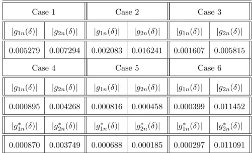
The simulation results of point-wise kernel estimation are reported in Tables 5.1 and 5.2, which consider six different parameter constellations for {ρ, ρi, λi,(δ, h)}:
Case 1 :ρ=ρ1=ρ2 = 0, λ1 =λ2=λ3 = 0, (δ, h) = ( 1 4, 1 6 ) ; Case 2 : ρ=ρ1 =ρ2 = 0, λ1=λ2 =λ3= 0, (δ, h) = ( 1 2, 1 3 ) ; Case 3 : ρ=ρ1 =ρ2 = 0, λ1=λ2 =λ3= 0, (δ, h) = ( 3 4, 1 2 ) ; Case 4 : ρ= 0.5, ρ1=−0.5, ρ2 = 0.5, λ1=λ2 =λ3 = 0.5, (δ, h) = ( 1 4, 1 6 ) ; Case 5 : ρ= 0.5, ρ1=−0.5, ρ2 = 0.5, λ1=λ2 =λ3 = 0.5, (δ, h) = ( 1 2, 1 3 ) ; Case 6 : ρ= 0.5, ρ1=−0.5, ρ2 = 0.5, λ1=λ2 =λ3 = 0.5, (δ, h) = ( 3 4, 1 2 ) .
Broadly speaking, |g1n(δ)| is smaller than |g2n(δ)|, which supports the asymptotic theory in Section 3 that g1n(δ) converges to zero at a faster rate than g2n(δ). The presence of endogeneity betweenxtandutdoes not impose a noticeable impact on the results, corroborating similar findings by Wang and Phillips (2009b) in the context of nonlinear cointegration models with a univariate regressor. The bias-corrected kernel method implies a second-order bias correction for gin(·), as shown in Proposition 4.1. We find that the corresponding values of|g∗1n(δ)|and|g∗2n(δ)|are slightly smaller than those for |g1n(δ)| and |g2n(δ)| reported in Tables 5.1 and 5.2, providing evidence of bias reduction and supporting the limit theory in Section 4.
Table 5.1: Absolute averages ofgin(δ) andgin∗ (δ) for the functional form M1
Case 1 Case 2 Case 3
|g1n(δ)| |g2n(δ)| |g1n(δ)| |g2n(δ)| |g1n(δ)| |g2n(δ)| 0.005279 0.007294 0.002083 0.016241 0.001607 0.005815
Case 4 Case 5 Case 6
|g1n(δ)| |g2n(δ)| |g1n(δ)| |g2n(δ)| |g1n(δ)| |g2n(δ)|
0.000895 0.004268 0.000816 0.000458 0.000399 0.011452
|g∗1n(δ)| |g2n∗ (δ)| |g1n∗ (δ)| |g2n∗ (δ)| |g1n∗ (δ)| |g∗2n(δ)| 0.000870 0.003749 0.000688 0.000185 0.000297 0.011091 Table 5.2: Absolute averages ofgin(δ) andgin∗ (δ) for the functional form M2
Case 1 Case 2 Case 3
|g1n(δ)| |g2n(δ)| |g1n(δ)| |g2n(δ)| |g1n(δ)| |g2n(δ)| 0.000302 0.026371 0.000504 0.002895 0.042893 0.059356
Case 4 Case 5 Case 6
|g1n(δ)| |g2n(δ)| |g1n(δ)| |g2n(δ)| |g1n(δ)| |g2n(δ)|
0.006109 0.005456 0.024125 0.049481 0.030661 0.069070
|g∗1n(δ)| |g2n∗ (δ)| |g1n∗ (δ)| |g2n∗ (δ)| |g1n∗ (δ)| |g∗2n(δ)| 0.005963 0.004695 0.023760 0.049477 0.030607 0.068099
Fig. 5.1 near here Fig. 5.2 near here
We next consider the case whereρ= 0.5,ρ1 = 0.5 andρ2= 0.5 andλi = 0.5 fori= 1,2,3. For
given h, we define the leave-one-out estimate
b ft(δ|h) = ∑n s=1,̸=t xsx′sK(s−nδ nh )+ ∑n s=1,̸=t xsysK(s−nδ nh ) ≡[f1tb (δ|h),f2tb (δ|h) ]′ , (5.8)
and the cross-validation function
CVn(h) = 1 n n ∑ t=1 [ yt−x′tfbt (t nh )]2 , (5.9)
and find an optimal bandwidth of the form bhcv = arg min h∈Hn CVn(h), (5.10) where Hn = [ n−1, n−23 log−1(n) ] . For δ > bhcv, define bδn = ⌊(δ−bhcv)n⌋, xbδn = ( x1,bδ n, x2,bδ(n) )′ , bbn(δ) = √1 nxbδn = 1 √ n ( x1,bδ n, x2,bδn )′ and qnb (δ) = [ x 1,bδn √ n∥bbn(δ)∥, x2,bδn √ n∥bbn(δ)∥ ]′ ≡ [bq1n(δ),bq2n(δ)]′. Let the transformed quantities g1n(δ) andg2n(δ) be again defined as in (5.4) and (5.5) but with qin(δ) and
pin(δ) replaced bybqin(δ) and pinb (δ), respectively, wherep1nb (δ) =q2nb (δ) andp2nb (δ) =−bq1n(δ).
The plots shown in Figs. 5.1 and 5.2 are based on 500 replications. These plots clearly show that the window of fluctuations of g1n(δ) is much narrower than that of g2n(δ), further corroborating the limit theory that the variance ofg1n(·) is smaller than that ofg2n(·).
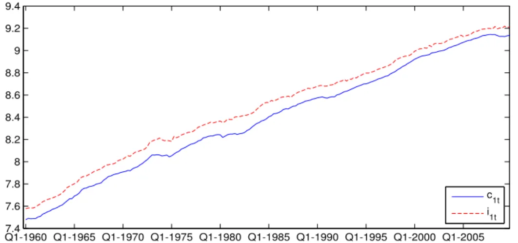
Example 5.2. We next apply the time varying coefficient model and estimation methodology to aggregate US data on consumption, income, investment, and interest rates obtained from Federal Reserve Economic Data (FRED)5. Two formulations are considered using data that were studied recently in Athanasopoulos et al (2011) using linear VAR and reduced rank regression methods.
Case (i) (Quarterly data over 1960:1–2009:3): c1t is log per-capita real consumption, i1t is log per capita disposable income, and rt is the real interest rate expressed as a percentage and calculated ex post by deducting the CPI inflation rate over the following quarter from the nominal 90 day Treasury bill rate.
Case (ii)(Quarterly data over 1947:1–2009:4): c2tis log per-capita real consumption,i2tis log per capita real disposable income, and zt is log per capita real investment.
The series are plotted in Figs. 5.3 and 5.4, which show that i1t, i2t and zt have trending components. In order to satisfy Assumption 1, we first eliminate the trends by introducing zjt =
ijt−µjtwithµj = n1∑nt=1(ijt−ij,t−1) forj= 1,2, andz3t=zt−µztwithµz= 1n
∑n
t=1(zt−zt−1).
Figs. 5.3(b), 5.3(c), 5.4(b) and 5.4(c) show that the differenced versions of zktfork= 1,2,3 andrt
all appear stationary, leading us to define yt=c1t,x1t=z1t andx2t=rtfor case (i), andyt=c2t,
x1t=z2tand x2t=z3tfor case (ii). Application of the nonparametric test in Gao and King (2011) for checking unit root nonstationarity givesp-values of 0.106 and 0.112 for x1t and x2t in case (i), and correspondingp-values of 0.132 and 0.116 forx1t and x2tin case (ii).
Fig. 5.3(a) near here Fig. 5.3(b) near here Fig. 5.3(c) near here Fig. 5.4(a) near here Fig. 5.4(b) near here Fig. 5.4(c) near here
In both cases, we fit the following model allowing for a time varying coefficient vector
yt=x′tf(t/n) +ut=x′tft+ut, t= 1,· · ·, n, (5.11)
where the regressors and coefficients are partitioned as xt = (x1t, x2t)′ and ft = (f1t, f2t)′. The
coefficient function f(·) = (f1(·), f2(·))′ is estimated by kernel weighted regression giving
b f(δ) = [ n ∑ t=1 xtx′tK(t−nδ nh )]+[∑n t=1 xtytK(t−nδ nh )] ≡[f1b(δ),f2b(δ) ] , (5.12)
where K(x) = 12I{−1≤x≤1} as in Example 5.1, over δ ∈(0,1],and the bandwidth h is chosen by cross-validation as described in (5.10). The nonparametric estimates of the two curvesfi(·) with their 95% confidence bands are shown in Figs. 5.5 and 5.6 for case (i), and in Figs. 5.7 and 5.8 for case (ii).
Fig. 5.5 near here Fig. 5.6 near here Fig. 5.7 near here Fig. 5.8 near here
The plots off1b(δ) andf2b(δ) are strongly indicative of nonlinear functional forms for the coeffi-cients in both cases, but also suggest that the functionsfi(δ) may be approximated by much simpler parametric functions gi(δ;θi), for some parametric valuesθi and pre-specified functionsgi(·;·). We
have done some pre–testing for all possible linear forms and other polynomial approximations be-fore we propose using the parametric polynomial approximations in equations (5.13)–(5.16) below. Therefore, for case (i), in Figs. 5.5 and 5.6, we also consider polynomial fitted specifications of the form: g1(δ;bθ1) =bθ01+ 6 ∑ j=1 b θj1δj, (5.13) g2(δ;bθ2) =bθ02+ 5 ∑ j=1 b θj2δj, (5.14) where bθ01 = 1.1036, bθ11 =−4.9534, bθ21 = 225.087, bθ31 = −63.983, bθ41 = 87.136, bθ51 =−60.191, b θ61 = 16.547; bθ02 = 0.4359, bθ12 = 4.577, bθ22 = −19.381, bθ32 = 41.327, bθ42 = −43.237 and b
θ52 = 17.001. Similarly, for case (ii), in Figs. 5.7 and 5.8, we consider the fitted polynomial
specifications: g1(δ;bθ1) =bθ01+ 3 ∑ j=1 b θj1δj, (5.15) g2(δ;bθ2) =bθ02+ 3 ∑ j=1 b θj2δj, (5.16)
where bθ01 = 1.5525, bθ11 =−3.0978, bθ21 = 3.7520, θb31 = −1.4718; bθ02 =−6.1002, bθ12 =−22.890,
b
θ22=−27.873 and bθ31= 11.100.
Figs. 5.5–5.8 show thatf1(δ) and f2(δ) are reasonably well captured by the parametric forms g1(δ;bθ1) and g2(δ;bθ2). Interestingly, lower order polynomial approximations are used in case (ii)
than those in case (i), even though the data cover a longer period in (ii) than (i). In case (ii) both regressors are macro aggregates (income and investment), and slower moving (i.e., less variable over time) functional responses might be expected. Case (i) involves the interest rate regressor, which displays greater volatility than the macro aggregates, so the functional responses are cor-respondingly more variable over the sample period and seem to require higher order polynomial approximations to adequately capture the nonparametric fits.
Standardt-tests show that all these coefficients are significant withp-values almost zero. Con-ventionalt-tests are robust to this type of parametric regression under nonstationarity, being equiv-alent to those from a standardised (weak trend) model of the form yt = ex′d,teg
(t n;θ0 ) +ut, where e xd,t= √xtn and eg (t n;θ0 ) = √ng(nt;θ0 )
giving the same p-values. A formal test of the polynomial specifications may be mounted to test the null hypothesis H0 : yt =x′tg
(t
n;θ0
)
+ut for a specific
parametric form g(·;θ0). The test statistic used to assess this (joint) null hypothesis is Ln(h),
which is defined in Appendix C of the online supplement. This statistic measures scaled departures of parametrically fitted functional elements from their nonparametric counterparts. A detailed development of this test statistic and discussions on its limit theory are provided in Appendix C.
For cases (i) and (ii), by using the block bootstrap method introduced in Appendix C of the online supplement, the calculatedp-values are 0.2937 and 0.3178,respectively, confirming that there is insufficient evidence to reject the null hypothesis H0 in both cases. In other words, a suitable
polynomial function provides a reasonable parametric approximation to each coefficient function
fi(δ) for both data sets over their respective sample periods.
This empirical example shows that while co-movement in macroeconomic data may well be supported by data inspection, linear cointegrating regressions with constant coefficients is often rejected in favor of models with time varying coefficients that allow the model to adapt to variations in the relationship over time. These variations are in many cases slowly moving and may be captured, as is done here, by kernel methods or by direct specifications in terms of simple basis functions like time polynomials.
6
Conclusions
Nonlinear cointegrated systems are of particular empirical interest in cases where the data are nonstationary and move together over time yet linear cointegration fails. Time varying coefficient models provide a general mechanism for addressing and capturing such nonlinearities, allowing for smooth structural changes to occur over the sample period. The present paper has explored a gen-eral approach to fitting these nonlinear systems using kernel-based structural coefficient estimation