Combining Generative and Discriminative
Representation Learning for Lung CT Analysis with
Convolutional Restricted Boltzmann Machines
Gijs van Tulder and Marleen de Bruijne
Abstract—The choice of features greatly influences the per-formance of a tissue classification system. Despite this, many systems are built with standard, predefined filter banks that are not optimized for that particular application. Representation learning methods such as restricted Boltzmann machines may outperform these standard filter banks because they learn a feature description directly from the training data. Like many other representation learning methods, restricted Boltzmann machines are unsupervised and are trained with a generative learning objective; this allows them to learn representations from unlabeled data, but does not necessarily produce features that are optimal for classification. In this paper we propose the convolutional classification restricted Boltzmann machine, which combines a generative and a discriminative learning objective. This allows it to learn filters that are good both for describing the training data and for classification. We present experiments with feature learning for lung texture classification and airway detection in CT images. In both applications, a combination of learning objectives outperformed purely discriminative or generative learning, increasing, for instance, the lung tissue classification accuracy by 1 to 8 percentage points. This shows that discriminative learning can help an otherwise unsupervised feature learner to learn filters that are optimized for classification. Index Terms—Representation learning, Restricted Boltzmann machine, Deep learning, Machine learning, Segmentation, Pattern recognition and classification, Neural network, Lung, X-ray imaging and computed tomography.
I. INTRODUCTION
Most methods for automated image classification do not work directly with image data, but first extract a higher-level description of useful features from the image. The choice of features determines a large part of the classification performance. Which features work well depends on the nature of the classification problem: for example, some problems require features that preserve and extract scale differences, whereas other problems require features that are invariant to those properties. Often, feature representations are based on standard filter banks of common feature descriptors, such as Gaussian derivatives that detect edges in the image. These
Copyright c⃝ 2016 IEEE. Personal use of this material is permitted. However, permission to use this material for any other purposes must be obtained from the IEEE by sending a request to [email protected]. This research is financed by the Netherlands Organization for Scientific Research (NWO).
G. van Tulder and M. de Bruijne are with the Biomedical Imaging Group, Erasmus MC, Rotterdam, The Netherlands. M. de Bruijne is also with the Department of Computer Science, University of Copenhagen, Denmark.
Code used for the experiments is available as supplementary material and athttp://vantulder.net/code/2016/tmi-ccrbm/.
predefined filter banks are not specifically optimized for a particular problem or dataset.
As an alternative to such predefined feature sets, represen-tation learning or feature learning methods [1] learn a high-level representation directly from the training data. Because this representation is learned from the training data, it can be optimized to give a better description of the data. Using this learned representation as the input for a classification system might give a better classification performance than using a generic set of features.
Most feature learning methods use unsupervised models that are trained with unlabeled data. While this can be an advantage because it makes it easier to create a large training set, it can also lead to suboptimal results for classification, because the features that these methods learn are not nec-essarily useful to discriminate between classes. Unsupervised feature learning tends to learn features that model the strongest variations in the data, while classifiers need features that discriminate between classes. If the variation between samples from the same class is much stronger than the variation between classes, feature learning probably produces features that capture primarily within-class variation. If those features do not represent enough between-class variation, they might give a lower classification performance.
This issue of within-class variation is relevant for many applications, including medical image analysis. For example, in disease classification, the differences between patients are often greater than the subtle differences between disease pat-terns. As a result, representation learners might learn features that model these between-patient differences, rather than those that improve classification.
In this paper we study the restricted Boltzmann machine (RBM), a popular representation learning model, as a way to learn features that are optimized for classification. The standard RBM does not include labels and is trained with an unsupervised, generative learning objective. The classification RBM [2], an extension of the standard RBM, does include label information and can also be trained with a discriminative learning objective. This discriminative learning objective opti-mizes the classification performance of the classification RBM. The generative and discriminative objectives can be combined to learn discriminative features that represent the data and are useful for classification.
We propose the convolutional classification RBM, which combines the classification RBM with the convolutional RBM, another extension of the standard RBM. The convolutional
RBM [3]–[6] uses the convolutional weight-sharing pattern from convolutional networks to learn small filters that are applied to every position in a larger image. This weight sharing makes learning more efficient and allows the RBM to model small features that occur in multiple areas of an image, which is useful for describing textures.
The ability to use both generative and discriminative learn-ing objectives distlearn-inguishes the classification RBM from many other representation learning methods. Unsupervised models such as the standard RBM are usually trained with only a generative learning objective. Supervised representation learn-ing methods, such as convolutional neural networks [7], are usually trained with only a discriminative learning objective. The classification RBM can be trained with a generative objective, a discriminative objective, or a combination.
We present experiments on lung tissue classification and airway detection. For the lung tissue classification experiments we used a dataset on interstitial lung diseases (ILD) [8] with CT images of 73 patients. Previously published tissue-classification experiments on this dataset used wavelets [9]– [12], local binary patterns [13], [14], bag-of-visual-words [15], [16], filter banks derived from the discrete Fourier transform [17], RBMs [18], [19] and convolutional networks [20].
We used RBMs to learn features for lung tissue classifica-tion. From the images, we first extracted 2D patches that we used to train RBMs with different mixtures of discriminative and generative learning. Using the RBM-learned representa-tions, we trained and evaluated classifiers that classify each patch in one of the five tissue classes. We compared those results with those of two standard filter banks.
We expected the effect of discriminative learning to become less important for larger representations (more hidden nodes in the RBM), because larger representations are more likely to contain sufficient discriminative features even without explicit discriminative learning. To study this effect, we performed airway detection experiments on lung CT images from the Danish Lung Cancer Screening Trial (DLCST) [21]. We used non-convolutional classification RBMs with different mixtures of discriminative and generative learning to learn features for this dataset. The non-convolutional RBMs allowed us to experiment with larger numbers of hidden nodes.
This paper extends our earlier workshop paper [22] in which we introduced the convolutional classification RBM and found that using a mixture of generative and discriminative learning objectives can produce features that improve classification results. In this paper, we present the results of more extensive experiments that confirm these preliminary conclusions.
The rest of this paper is organized as follows. Section II gives a brief overview of other relevant representation learning approaches. Section III describes the RBM and its learning algorithm. Section IV introduces the datasets and the ex-periments. Section V describes the results. We end with a discussion andconclusion.
II. RELATED WORK
Representation learning methods have been used for tissue classification in lung CT before. In experiments similar to
those presented in this paper and using the same ILD dataset, Li et al. [18] used RBMs to extract features. Whereas we use classification RBMs with convolution to learn small filters, Li et al. trained standard (non-convolutional) RBMs on small subpatches extracted from the patch that is to be classified. In later work [19] on the same dataset, Li et al. reported that con-volutional neural networks gave a slightly better performance than standard RBMs. Gao et al. [20] used convolutional neural networks to classify full slices from the ILD dataset, without requiring manually annotated ROIs. Schlegl et al. [23] also used convolutional neural networks to classify lung tissue in a different lung CT dataset.
Convolutional neural networks have also been used in other applications of lung CT, such as the detection of lung nodules and lymph nodes. In an early application of convolutional neu-ral networks, Lo et al. [24], [25] trained a network to reject or confirm potential lung nodules selected in a preprocessing step. More recently, Shen et al. [26] used multi-scale convolutional networks to compute features for lung nodule classification. Kumar et al. [27] used multi-layer autoencoders to extract features for the classification of lung nodules. Roth et al. [28] proposed a so-called 2.5D convolutional neural network that samples multiple 2D orthogonal views to detect lymph nodes in lung CT images.
To our knowledge, classification RBMs have not been applied to lung CT images before, and there are only a few applications in other types of medical image analysis. Shin et al. [29] used classification RBMs to detect micro-calcifications in digitized mammograms. Berry and Fasel [30] used translational deep Boltzmann machines, which are related to classification RBMs, to analyze ultrasound images of the tongue. Schmah et al. [31] analyzed fMRI data with RBMs with generative and discriminative learning.
III. RESTRICTEDBOLTZMANN MACHINES A. Standard RBM
The restricted Boltzmann machine is a probabilistic neural network that learns the probability distribution of its inputsv and a hidden representation h. The visible nodesv represent the voxels of an input patch. To model the patches from our lung CT images, we use Gaussian visible nodesvand binary hidden nodesh(see [32] for a description of these node types). Each visible nodevihas an undirected connection with weight Wij ∈R to each hidden nodehj. The model also includes a bias bi ∈ R for each visible node vi and a bias cj ∈ R for each hidden nodehj. Together, the weights and biases define the energy function of the RBM:
E(v,h) =∑ j (vi−bi)2 2σ2 i −∑ i, j vi σi Wijhj− ∑ j cjhj , (1)
where σi is the standard deviation of the Gaussian noise of visible node i. We normalize the training patches such that σi = 1. The joint distribution of the input v and hidden representationhis defined as
P(v,h) = exp (−E(v,h))
hiddenh
inputv labely
W U
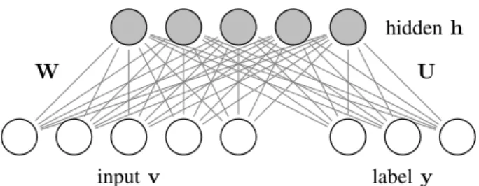
Fig. 1. Schematic view of the classification RBM, which adds a set of label nodes to the visible layer of the standard RBM. The label nodes are connected to the input nodes through the hidden layer.
where Z is a normalization constant. The conditional proba-bilities for the hidden nodes given the visible nodes and vice versa are P(hj|v) = sigm(∑ i Wijvi+cj)and (3) P(vi|h) =N(vi|∑ j Wijhj+bi, σi2), (4)
where sigm (x) = 1+exp(1−x) is the logistic sigmoid function and N(xµ, σ2) is a Gaussian probability density function with mean µand varianceσ2, evaluated at x.
B. Classification RBM
The standard RBM is an unsupervised model. The classi-fication RBM [2] extends the standard RBM by adding a set of label nodes to the visible layer (Figure 1). This allows the RBM to learn the joint probability of the input, the hidden representation, and the label. The label nodes use a one-hot coding, where there is one nodeyk per class such thatyk = 1 if the sample belongs to class k andyk = 0 otherwise. The label nodes have a bias dk ∈ R and are connected to the hidden nodes, with a connection with weightUkj∈Rbetween label node yk and hidden node hj. The energy function of a classification RBM with Gaussian visible nodes is
E(v,h,y) =∑ j (vi−bi) 2 2σ2 i −∑ i, j vi σiWijhj− ∑ j cjhj −∑ k, j ykUkjhj−∑ k dkyk . (5)
The energy function defines the distribution
P(v,h,y) =exp (−E(v,h,y))
Z (6)
and the conditional probabilities
P(hj|v,y) = sigm(∑ i Wijvi+∑ k Ukjyk+cj)and (7) P(yk|h) = sigm(∑ j Ukjhj+ck). (8)
The visible nodes and the label nodes are not connected, so the expression for P(vi|h) is unchanged from the standard
RBM. The posterior probability for classification is
P(y|v) = (9)
exp (
dy+∑jsoftplus(cj+Ujy+∑iWijvi) ) ∑ y∗exp ( dy∗+∑jsoftplus(cj+Uy∗j+ ∑ iWijvi) ),
where softplus(x) = log (1 + exp (x)). This definition only works for RBMs with binary hidden nodes: it implicitly sums over all possible states of the hidden layer, which can be done efficiently if each hidden node can take one of only two values [2].
C. Generating samples and classifying with RBMs
RBMs are probabilistic models that define the activation probability for each node given all other nodes. In practice, computing the probability of a particular statev,his impos-sible, because the normalization constant or partition function Z in the energy function is infeasible to compute for any but the smallest models. However, since it is possible to compute the conditional probabilities, we can still use Gibbs sampling to sample from the model. Gibbs sampling alternately samples from the hidden and visible layers. Given the visible and label nodes, the new state of the hidden nodes can be sampled using the distributionp(ht|vt, yt). Then, keeping the hidden nodes fixed, the new activation of the visible and label nodes can be sampled fromp(vt, yt|ht). This can be repeated for several iterations, until the model converges to a stable state. For simplicity, we used a fixed number of iterations in our experiments.
Classifying a patch using the classification RBM is more straightforward. We input the patch values in the visible layer v and use Equation (9) to compute the posterior probability P(y|v)for each class. We assign the label of the class with the highest posterior probability.
D. Learning objectives
At training time, the weights and biases of the standard RBM are chosen to optimize the generative learning objective logP(vt), the probability distribution of each input imaget. The classification RBM can be trained with the generative learning objective logP(vt, yt), which optimizes the joint probability distribution of the input image and the label. A classification RBM can also be trained with the discriminative objective logP(yt|vt), which only optimizes the classifica-tion and does not try to optimize the likelihood of the input image. Larochelle et al. [2] suggest a hybrid objective
βlogP(vt, yt) + (1−β) logP(yt|vt), (10) whereβ ∈[0,1]is the proportion of generative learning. We will use this objective with different values forβin our feature learning experiments.
The normalization constant or partition functionZ makes it unfeasible to compute the gradient of the generative learning objective. Instead, we use Gibbs sampling and contrastive divergence [32] to estimate the stochastic gradient descent updates for our RBMs. Contrastive divergence provides an
· · ·
W1 W2 WM
WM
h1 h2 hM
input image v
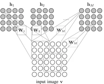
Fig. 2. Schematic view of the convolutional RBM, which uses a convolutional weight-sharing arrangement to reduce the number of connection weights.
efficient approximation for the gradient-based updates to the weights and biases.
Classification RBMs are slightly more computationally ex-pensive than unsupervised RBMs, because they use an ad-ditional discriminative learning objective and include extra weights to connect the label nodes. In practice however, we find that the classification RBMs are not much slower than the unsupervised RBMs, because the additional complexity from the discriminative components is small compared with the other parts of the RBM. The number of labels and the number of associated weights is usually much smaller than the number of connections between the visible and hidden layers, and the discriminative learning objective can be computed much faster than the generative objective, which requires contrastive divergence and Gibbs sampling.
E. Convolutional RBM
Designed to model complete images instead of small patches, convolutional RBMs [3]–[6] use the weight-sharing approach from convolutional neural networks. Unlike convo-lutional neural networks, convoconvo-lutional RBMs are generative models and can be trained in the same way as standard RBMs. In a convolutional RBM, the connections share weights in a pattern that resembles convolution, with M convolutional filters Wmthat connect hidden nodes arranged inM feature maps hm (Figure 2). The connections between the visible nodes and the hidden nodes in map m use the weights from convolution filter Wm, such that each hidden node is connected to the visible nodes in its receptive field. The visible nodes share one bias b; all hidden nodes in map m share the bias cm. With the convolution operator ∗ we define the probabilities P(hmij|v)= sigm((W˜m∗v)ij+cm ) and (11) P(vij|h) =N(vij (∑ m Wm∗hm ) ij+b, 1 ) , (12)
where W˜m is the horizontally and vertically flipped filter Wm, and·ij denotes the voxel on location(i, j).
feature maps h1,h2, . . . ,hM
input image v
labelsy
W1, . . . ,WM
U
Fig. 3. Schematic view of the convolutional classification RBM. The connection weightsUare shared between all nodes in a feature map.
Convolutional RBMs can produce unwanted border effects when reconstructing the visible layer, because the visible nodes near the borders are only connected to a few hidden nodes. We pad our patches with voxels from neighboring patches, and keep the padding voxels fixed during the iter-ations of Gibbs sampling.
F. Convolutional classification RBM
We use the convolutional classification RBM we introduced in our workshop paper [22]. This RBM includes visible, hidden and label nodes (Figure 3) and can be trained in a discriminative way. The visible nodes are connected to the hidden nodes using convolutional weight-sharing, as in the convolutional RBM, and the hidden nodes are connected to the label nodes, as in the classification RBM. In our patch-based texture classification problem, the exact location of a feature inside the patch is not relevant, so we use shared weights to connect the hidden nodes and the label nodes. All connections from a label node yk to a hidden node hm
ij in map m share the weightUkm. The activation probabilities are
P(yk|h) = sigm(∑ m Uym∑ i,j hmij +dk ) and (13) P(hmij|y)= sigm((W˜m∗v ) ij+ ∑ k Ukmyk+cm ) . (14)
Since the label nodes are not connected to the visible nodes, the probability for the visible nodes is unchanged from the convolutional RBM.
IV. EXPERIMENTS
We present experiments on lung CT images for two ap-plications and datasets: lung tissue classification and airway centerline detection. On the lung tissue dataset, we studied the effects of combining generative and discriminative learning objectives. On the airway dataset, we explored how these effects change if the representation is larger (more hidden nodes).
Fig. 4. First dataset. Example from the interstitial lung disease scans. The annotation (right) shows an ROI (red) marked as micronodules.
A. Dataset 1: Lung tissue classification
1) Purpose: This set of experiments studied the effect of combining generative and discriminative learning objectives. We trained RBMs with purely discriminative (β = 0), with purely generative (β = 1), and with mixed learning objectives. We then used the RBM-learned filters to compute feature vectors and train a classifier. The classification accuracy gives an indication of the quality of the learned representations.
2) Data: We used a publicly available dataset on interstitial lung diseases (see [8] for a description). In this texture classification problem with 73 scans from different patients, we classify patches of five types of lung tissue. The in-plane voxel size varies between 0.4−1 mm, with a slice thickness of 1−2 mm and inter-slice spacing of 10−15mm. The dataset provides hand-drawn 2D ROIs with labels for a subset of slices in each scan (Figure4). Following other work on this dataset (e.g., [11]), we extracted patches of 32×32 voxels along a grid with a16-voxel overlap. We include a patch if at least 75%of the voxels belong to the same class. We classify patches from the five most common tissue types in the dataset (healthy tissue: 22%, emphysema: 3%, ground glass: 16%, fibrosis: 15%, micronodules: 44% of the patches).
3) Experiments: We used the convolutional RBM, with and without labels, to learn filters from the patches in the lung tissue dataset. We then used these filters in a convolution to get feature maps for each of the patches in the dataset. For each feature map, we computed a histogram of the feature activations, using adaptive binning [33] over all patches in the training set. The concatenated histograms form the feature vector for each patch. We trained random forest classifiers to classify each patch in one of the five tissue classes.
4) Normalization: We trained the RBMs on normalized patches, with each patch normalized to zero mean intensity and unit standard deviation. We used unnormalized patches to compute the feature maps and histograms, to preserve the intensity differences between patches.
5) Baselines: We compare the results of the RBMs with those of several other methods. First, we show the performance of using random filters, using the same convolutional architec-ture but without optimizing the filter weights (see Figure5for an example). The results of random filters help to separate the contribution of feature learning from that of the convolutional
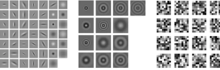
Fig. 5. Two filter banks: Leung-Malik (left) and Schmid (middle), generated with the code fromhttp://www.robots.ox.ac.uk/∼vgg/research/texclass/filters. html. An example of random filters (16 filters of8×8voxels) is shown right.
architecture [34]. We also compare the RBM-learned filters with two of the frequently-used standard filter banks discussed by Varma and Zisserman [35]: the Leung-Malik and Schmid filter banks (Figure 5). The filter bank of Leung and Malik [36] is a set of Gaussian filters and derivatives, with 48 filters of32×32voxels. The filter bank of Schmid [37] has 13 filters of 31×31voxels with rotation-invariant Gabor-like patterns. 6) Implementation and parameters: We implemented the RBMs in Python using the Theano library [38] and used the random forest implementation from Scikit-learn [39]. To optimize the learning parameters for the RBMs and random forests, we performed a grid search using nested cross-validation with patches from the same scan grouped in the same fold. We tried various learning rates for the RBM (10−3 to10−9). For the random filters, we chose the best filter set out of five random initializations. We used2 to8 bins in the adaptive binning step. For the random forests, we varied the number of trees (10 to 200) and the maximum number of features (1to256), and used Scikit-learn’s default parameters for the other settings.
The initial values for the connection weightsWof the RBM were sampled from a normal distribution with mean 0 and standard deviation10−6. The initial values for the connection weights U of the classification RBMs were sampled from a uniform distribution [−10−6,10−6]. All biases had the initial value 0. During stochastic gradient descent we used a minibatch size of 5, with one Gibbs sampling step for contrastive divergence.
7) Cross-validation: Almost all scans have manually-drawn ROIs for only one tissue type. We organized the scans in five folds, of 15 or 14 scans each, while trying to create a similar class distribution in each fold. We present the validation accuracy over all five folds. In each cross-validation step we used one fold for testing and the remaining four folds for classifier training and parameter tuning. For each fold, we computed the mean accuracy over all patches. Within each cross-validation step, we optimized the RBM and random forest parameters using nested cross-validation with one validation and three training folds. We used the parameters that gave the best accuracy over the four folds to train a classifier on the full training set, which we then used to classify the patches from the scans in the test fold.
We report the mean classification accuracy over all five folds in the cross-validation. We used the Wilcoxon signed-rank test to test for significant differences between methods (p <0.05). In these tests we compared the classification accuracy per scan
Fig. 6. Second dataset. In the airway dataset, we extract patches at the airway centerline (green) and non-airway samples (red) close to the airway.
(73 measurements per method).
B. Dataset 2: Airway centerlines
In our second set of experiments we explored the influence of the size of the representation – the number of hidden nodes in the RBM. Since it was computationally unfeasible to train the convolutional RBM with a very large number of filters, we performed these experiments on a different problem with a classification RBM without convolution. We used 40 lung CT scans from 20 participants of the Danish Lung Cancer Screening Trial (DLCST) [21]. The voxel size is approximately 0.78×0.78×1 mm. Using the output of an existing segmentation algorithm [40] to find the airways (Figure6), we extracted patches of16×16voxels at the center point of airways with a diameter of 16 voxels or less. For each airway patch, we created a non-airway sample by extracting a patch at a random point just outside the outer airway wall. We selected a random subset of 500 patches per scan. We used 15 subjects (30 scans, 15 000patches) as our training set and 5 subjects (10 scans, 5 000 patches) for testing.
The implementation and parameters were similar to those for the tissue classification dataset, with a few differences. Because the airway in this dataset is always in the center of the patch, we could use RBMs without convolution to learn a representation. We used between 1 to 256 nodes in the hidden layer. We used the scans from the training set to train classification RBMs and standard RBMs. Using the representation in the hidden layer of the RBM to create the feature vectors, we trained random forests to classify airway and non-airway voxels. We optimized the parameters of the random forests using cross-validation on the training set. We report the classification accuracy of the classification RBMs and of the random forests on the test set.
V. RESULTS
A. Filters
Figure 7 shows filters learned by the RBM from the lung tissue classification dataset, for various mixtures of generative and discriminative learning. Because of the different random initializations, each set of filters looks different, but we ob-served no consistent visual difference between filters learned
β= 0 β= 0.01 β= 0.1 β= 1
discriminative mixed generative
Fig. 7. Example filters learned from the ILD dataset, with different mixtures of generative and discriminative learning (16 filters of8×8voxels).
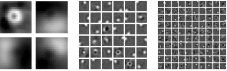
Fig. 8. Three filter sets learned from the airway data: 4, 36 or 100 filters of 16×16voxels, learned with a mix of discriminative and generative learning (β= 0.01).
with discriminative or generative learning. These filters are apparently useful for modeling and classifying the textures in the data, but there are no recognizable structures. With the non-convolutional RBM, which we used for the airway dataset, the filters show more recognizable structures (Figure 8). The filters show circular structures that resemble the airways in the training set: a centered, dark circle to represent the airway, and white blobs that could represent the vessel that is often next to the airways. With a small number of filters, the RBM learned more general filters, whereas an RBM with more filters learned filters that can represent more specific structures.
B. Random forest classification
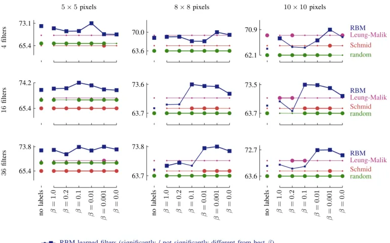
Figure 9 shows the random forest classification results comparing RBM-learned filters with different filter banks. The classification accuracy achieved using the RBM-learned filters with the best β was better than that using random filters or one of the predefined filter banks. Random filters and, in most cases, the Schmid filters performed significantly worse than the RBM-learned filters. The difference with the Leung-Malik filter bank was often not significant. The best performance was achieved using16filters of5×5 voxels.
Pure generative or discriminative learning usually performed worse than a mixture of learning objectives. The effects of using different values forβ were most visible with the larger filters. At most filter sizes, except for very small or very few filters, using a combination of generative and discriminative learning seems to give better results than using purely gen-erative or discriminative learning. The classification accuracy increases as β decreases, until it decreases again when there is too much discriminative learning, which increases the risk of overtraining.
C. RBM classification
We also looked at the classification performance of the RBM itself, using Equation (9) to compute the posterior probability
5×5pixels 4 filters 73.1 65.4 16 filters 74.2 65.4 36 filters 73.8 65.4 no labels β = 1 . 0 β = 0 . 2 β = 0 . 1 β = 0 . 01 β = 0 . 001 β = 0 . 0 8×8pixels 70.0 63.6 73.6 63.7 73.8 63.7 no labels β = 1 . 0 β = 0 . 2 β = 0 . 1 β = 0 . 01 β = 0 . 001 β = 0 . 0 10×10pixels 70.9 62.1 Leung-Malik Schmid random RBM 73.5 63.7 Leung-Malik Schmid random RBM 72.7 63.6 no labels β = 1 . 0 β = 0 . 2 β = 0 . 1 β = 0 . 01 β = 0 . 001 β = 0 . 0 Leung-Malik Schmid random RBM
RBM-learned filters (significantly / not significantly different from best β)
Leung-Malik filters (not significantly / significantly different from RBM-learned filters)
Schmid filters (not significantly / significantly different from RBM-learned filters)
random filters (not significantly / significantly different from RBM-learned filters)
Fig. 9. Random forest classification accuracy on the lung tissue classification dataset, for different feature representations. Large squares indicate RBM results that are not significantly different (p <0.05) from the best RBM result for that network configuration. Large circles indicate results that are significantly different from the RBM result at that β. (All significance values were computed using Wilcoxon signed-rank tests comparing the per-scan classification accuracies.)
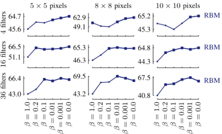
for each class. The accuracy of the RBM was always lower than that of the random forests (Figure 10). With just the generative learning objective, the classification accuracy of the RBM was poor, presumably because this model optimized only for representation and not for classification. Using the discriminative learning objective improved the accuracy, but it was still significantly lower than that of a random forest trained on the RBM hidden layer. One reason may be that the classification model of the RBM is much simpler than that of the random forests. The RBM has a linear decision function (given the state of the hidden layer) and does not compute histograms of the feature activations. In addition, the RBM optimization may be complicated by the fact that the RBM optimizes two things at the same time (representation and classification).
D. Influence of the size of the representation
We explored the effects of the filter size and the number of filters on the classification performance. We expected that discriminative learning would become less important as the number of filters increases, because a larger representation
is more likely to include discriminative features even with generative learning.
Figure9 shows the results for multiple network configura-tions with different filter sizes and numbers of filters on the tissue classification problem. There seems to be a connection between the number of filters and the point at which the accu-racy increases. With more filters, more discriminative learning (a smaller β) is needed. This could be a consequence of the implementation of the gradients of the energy function: in an RBM with many filters, the values in the energy function (and the corresponding gradients) might be larger than when the number of filters is smaller. The number of filters influences the gradient for the generative learning objective, but not the discriminative objective. To achieve the right balance between discriminative and generative learning, theβshould be smaller for smaller number of filters to compensate for the larger gradients.
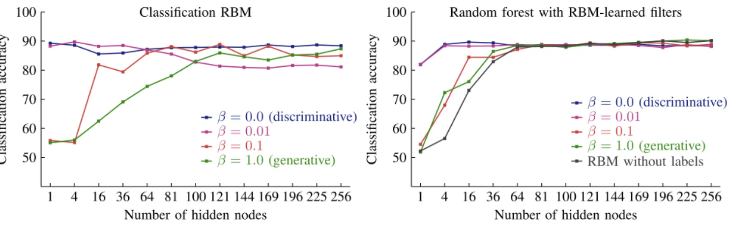
For a closer look at the effect of the representation size, we performed additional experiments with non-convolutional RBMs on the airway dataset (Figure 11). On this dataset, using only or mostly discriminative learning generally gave the best results. The performance of generative learning depended
on the number of hidden nodes. With only a few hidden nodes, generative learning performed worse than discrimina-tive learning. As we increased the size of the representation, the gap between generative and discriminative learning almost disappeared. This seems to agree with our hypothesis that at the smaller representations, the discriminative objective helps to learn discriminative features, whereas the generative objective produces features that are useful for representation but are less discriminative. As we increased the number of hidden nodes, generative learning produced enough features to also include some of the discriminative features.
E. Comparison with our previous results
The results in this paper are largely in agreement with the results from our previous paper [22]. There are a number of differences with respect to our previous work. We performed more extensive experiments, with cross-validation that used all available scans. We previously used a fixed training and test set. Because the differences in classification accuracy between individual scans are large, this makes it hard to directly compare the results of these and our previous experi-ments. In general, the classification performance in these new experiments was better than in our previous experiments.
There are also some technical differences. Previously, we used support vector machines with linear and radial basis function (RBF) kernels. In the extended experiments discussed here, we used random forest classifiers; these classifiers were easier to train, which made it possible to do a larger parameter search.
A surprising difference with our previous results was the improved performance of the Leung-Malik and Schmid filter banks. Previously, both filter banks performed worse than the random filter sets. In our current experiments we used larger training sets and used cross-validation to measure the mean classification accuracy over all scans, instead of using a fixed test set. Since there are large differences between scans, these new results may provide a better estimate of the actual performance of the standard filter banks.
Despite these differences, the effect of the two learning objectives in the current experiments largely agrees with the results of our previous experiments. In both cases, using a mixture of generative learning gave a better performance than using only one of the two objectives. The classification performance of the RBM is also similar to what we found earlier: lower than the SVM or random forest.
VI. DISCUSSION
We have shown how the classification RBM can be used to learn useful features for medical image analysis, achieving a mean classification accuracy that was better than or close to that achieved using a predefined set of features. To get good classification results in feature learning, it is important to use the right learning objective. We found that adding label information and discriminative learning to the standard RBM helps to produce filters that improve performance. In some cases pure discriminative learning worked best, but in most cases a mixture with generative learning gave better results.
5×5pixels 4 filters 64.7 45.6 16 filters 66.5 51.1 36 filters 66.4 43.0 β = 1 . 0 β = 0 . 2 β = 0 . 1 β = 0 . 01 β = 0 . 001 β = 0 . 0 8×8pixels 62.9 49.1 65.3 46.3 69.5 43.2 β = 1 . 0 β = 0 . 2 β = 0 . 1 β = 0 . 01 β = 0 . 001 β = 0 . 0 10×10pixels 65.2 45.3 RBM 64.8 44.3 RBM 67.5 40.8 β = 1 . 0 β = 0 . 2 β = 0 . 1 β = 0 . 01 β = 0 . 001 β = 0 . 0 RBM
Fig. 10. The RBM classification accuracy on the lung tissue classification dataset, for different feature representation methods. Large squares indicate results that are not significantly different from the best result for that network configuration. (All significance values were computed using Wilcoxon signed-rank tests comparing the per-scan classification accuracies.)
The results show that RBM-learned filters have an advantage over random filters and two standard filter banks.
Random filters performed quite well in our experiments, although they generally performed worse than the filter banks and RBM-learned filters. The surprisingly good performance of random filters has already been noted in the literature [34]. When the number of filters is large enough, convolution with random filters can provide useful features to train a classifier. The performance of random filters is a useful baseline because it allows us to separate the contribution of the convolutional architecture from that of the feature learning algorithm. The performance difference between learned and random filters indicates that the improvement is not just an effect of using a convolution operator with a number of arbitrary filters.
A. Results on the ILD dataset
The ILD dataset [8] used in our experiments was also used in other papers. We will give a brief overview of the techniques and the results before comparing them with our own.
Depeursinge et al., the providers of the dataset, used wavelet transforms and intensity and gradient features [9]–[11] to classify tissue patches. They also used this tissue classification system as a component of a larger image retrieval system [12]. From the same group, Foncubierta-Rodr´ıguez et al. [15] proposed a retrieval system based on visual words. The five-class five-classification accuracy reported in these papers ranges between76.1%and80.8%.
Song et al. used texture, intensity and gradient features, combined with features based on rotation-invariant Gabor-local binary patterns and histogram of oriented gradients. Song et al. [13] first used a dictionary to approximate the test patch using training patches and then used the approximation error to classify the patch. They combined this approach with a large-margin local estimate method to cluster example patches [14], with a reported classification accuracy of 86.1%. A related method [41], also based on clustering, provided a 85.8% classification accuracy. Earlier, the same authors also used local binary patterns [42] and boosting [43].
β= 0.0(discriminative)
β= 0.01 β= 0.1
β= 1.0(generative)
Number of hidden nodes
Classification accurac y Classification RBM 1 4 16 36 64 81 100 121 144 169 196 225 256 50 60 70 80 90 100 β= 0.0 (discriminative) β= 0.01 β= 0.1 β= 1.0 (generative) RBM without labels
Number of hidden nodes
Classification
accurac
y
Random forest with RBM-learned filters
1 4 16 36 64 81 100 121 144 169 196 225 256 50 60 70 80 90 100
Fig. 11. Classification accuracy on the airway dataset, showing the influence of the number of hidden nodes in the RBM representation on the classification accuracy, for different mixtures of discriminative and generative learning. The graph on the left shows the classification accuracy of the classification RBM. The graph on the right shows the classification accuracy of a random forest using the RBM-learned filters.
Asherov et al. [16] used bags of visual words to classify patches, reporting an accuracy of 79%. Anthimopoulos et al. [17] used filter banks derived from a discrete cosine transform, which performed better than Leung-Malik, Schmid, Gabor and MR8 filters. Dash et al. [44] presented segmenta-tion methods using Markov random fields, Gaussian mixture models and mean-shift algorithms.
Several papers applied representation learning methods to the ILD dataset. Li et al. presented experiments using RBMs to extract features [18], which gave a classification accuracy of 77%. In a later comparison, Li et al. reported that convolu-tional neural networks gave a slightly better performance [19] (no accuracy given). Gao et al. [20] used convolutional neural networks to classify full slices, without requiring manually annotated ROIs. Their patch-based classification showed a classification accuracy of87.9%.
It is difficult to compare the results of our experiments with those in the previously published studies. Although many papers use a similar approach to extract patches, there are differences in cross-validation procedures and in the number of patches. Overall, our classification results seem to be in the same range, but worse than the state-of-the-art results [14]. Part of this may be due to a difference in training set size – the papers with better results use leave-one-patient-out validation (e.g., [14]), whereas we used five-fold cross-validation for computational reasons. Other differences may also be important, such as the number of features (we used a relatively small number of filters, also for computational reasons) and the amount of post-processing.
B. How much discriminative learning is required?
There is no single optimal mixture of discriminative and generative learning. The optimal choice forβ depends on the number and size of the filters, on the application, and on the dimensions of the data. The results from our lung tissue classification experiments (Figure 9) show that the influence of β is strongest for RBMs with larger filters, with lower β (more discriminative learning) giving a better classification accuracy. The effect of the number of filters or the number of hidden nodes is more easily visible in the results of the
airway centerline experiments (Figure 11), which show that discriminative learning becomes less important for models with more hidden nodes. Some of these trends will be a result of the definition of the generative learning objective, which is derived from an energy function that tends to be larger for RBMs with many connections (more or larger filters). The remainder of the effect may be explained by the difficulty of finding a set of discriminative features. This difficulty is influenced by two factors: the number and the size of the filters. A model with only a few filters may require more discriminative learning than a model with many filters: a large set of filters is more likely to contain some that are useful for classification even if the filters are learned with generative learning, but with a small set of filters it is necessary to be selective. Similarly, a model with large filters may require more discriminative learning than a model with small filters, because the model with larger filters has a larger search space: a model with larger filters can find more different filters, which makes it more important to be selective.
The optimalβ also depends on the application and dataset. If it is difficult for the RBM to learn the classification rule, such as in our lung tissue classification experiments, a mixture with generative learning proved to work better than purely discriminative learning. On a somewhat easier problem such as our airway centerline data, purely discriminative learning often gave good results as well.
Finally, the optimal mixture depends on the dimensions of the input data. In this paper, we chose to do feature learning and classification in 2D, because the lung tissue data that we used in our experiments is highly anisotropic and has only 2D annotations. However, given the right training data, the methods discussed in this paper can be extended to 3D. Having 3D inputs increases computational complexity, which is sometimes a reason to use pseudo-3D, as in [28] where 3D data is modeled with a set of orthogonal 2D planes. If real 3D is used, it is important to limit the number of filters. At the same time, a 3D model will require more filters to model the training patches effectively. In those cases a mixture of generative and discriminative learning could help to learn fewer but better filters.
C. Further considerations
Since the mixture of generative and discriminative learning objectives can improve performance for RBMs, it might be interesting to try this combination for other representation learning methods, such as convolutional neural networks, deep belief networks or deep Boltzmann machines. However, this requires definitions for both the generative and the discrim-inative objective. Defining such mixed learning objectives could be difficult for many multi-layer networks. In this paper we used single-layer RBMs, for which it is straightforward to combine discriminative and generative learning objectives. A similar combined objective could be defined for deep Boltzmann machines – which are similar to RBMs but have multiple layers that are trained at the same time – by adding a label component to the top layer and using a combined learning objective to update the weights in all layers of the model. This approach only works for models in which all layers can be trained at the same time using both learning objectives. In practice, deep Boltzmann machines are often initialized with layer-wise pre-training [45], and since this initialization influences the final solution, it may be important to include a discriminative objective in this first phase as well. A similar problem applies to deep belief networks, which consist of stacked RBMs that are also trained layer-by-layer [46]. In both approaches, including a temporary label component while training the lower layers might provide a solution. In convolutional neural networks, all layers are trained at the same time, but usually only using a discrimina-tive objecdiscrimina-tive. Unsupervised generadiscrimina-tive pre-training can give good results [47] by using a generative learning objective to initialize weights that are then refined with a discriminative learning objective, but this approach separates the generative and discriminative training. This may give worse results than training with a combined objective. Classification RBMs have the advantage that they can be trained with generative and discriminative objectives simultaneously.
Although we found that learned filters could outperform the predefined filter banks in our experiments, the predefined filter banks had one obvious advantage: they did not have to be learned. Learning the filters can take some time, depending on the implementation, the hardware and the number and size of the filters (in our tissue classification experiments, training one RBM with 16 filters of8×8pixels took approximately 4 days using two CPU cores). The runtime of the classification RBMs was not longer than that of the standard RBMs. Once the features have been learned, however, computing features and training and applying the classifiers does not require more time than with predefined filter banks.
VII. CONCLUSION
We presented experiments with convolutional classification RBMs, which we trained with generative and discriminative learning objectives. Feature learning is usually done with a purely generative learning objective, which favors a represen-tation that gives the most faithful description of the data but is not always the representation that is best for the goal of the system. This paper showed how the standard generative
learning objective of an RBM can be combined with a dis-criminative learning objective. In our experiments, evaluating the classification accuracy of random forests using RBM-learned features, we found that a mixture of discriminative and generative learning objectives often gave a better classification accuracy than generative or discriminative learning alone. The features learned with the mixed learning objective gave better results than several standard filter banks. Our results suggest that adding discriminative learning is most useful when learning smaller representations, with fewer filters or hidden nodes.
ACKNOWLEDGMENT
Data for the lung tissue classification experiments was provided by the University Hospitals of Geneva [8]. Data for the airway centerline experiments was provided by the Danish Lung Cancer Screening Trial [21].
REFERENCES
[1] Y. Bengio, A. Courville, and P. Vincent, “Representation Learning: A Review and New Perspectives,” Universit´e de Montr´eal, Tech. Rep., 2012.
[2] H. Larochelle, M. Mandel, R. Pascanu, and Y. Bengio, “Learning Al-gorithms for the Classification Restricted Boltzmann Machine,”Journal of Machine Learning Research, vol. 13, pp. 643–669, Mar. 2012. [3] G. Desjardins and Y. Bengio, “Empirical Evaluation of Convolutional
RBMs for Vision,” Universit´e de Montr´eal, Tech. Rep., 2008. [4] M. Norouzi, M. Ranjbar, and G. Mori, “Stacks of Convolutional
Re-stricted Boltzmann Machines for Shift-Invariant Feature Learning,” in
IEEE Conference on Computer Vision and Pattern Recognition, 2009. [5] H. Lee, R. Grosse, R. Ranganath, and A. Y. Ng, “Convolutional
deep belief networks for scalable unsupervised learning of hierarchical representations,” in ICML, New York, New York, USA, 2009, pp. 609–616.
[6] ——, “Unsupervised learning of hierarchical representations with convolutional deep belief networks,” Communications of the ACM, vol. 54, no. 10, pp. 95–103, Oct. 2011.
[7] Y. LeCun, L. Bottou, Y. Bengio, and P. Haffner, “Gradient-based learning applied to document recognition,” Proceedings of the IEEE, vol. 86, no. 11, pp. 2278–2324, Nov. 1998.
[8] A. Depeursinge, A. Vargas, A. Platon, A. Geissbuhler, P.-A. Poletti, and H. M¨uller, “Building a reference multimedia database for interstitial lung diseases,”Computerized Medical Imaging and Graphics, vol. 36, no. 3, pp. 227–38, Apr. 2012.
[9] A. Depeursinge, A. Foncubierta-Rodr´ıguez, D. Van de Ville, and H. M¨uller, “Lung Texture Classification Using Locally-Oriented Riesz Components,” inMICCAI, 2011, pp. 231–238.
[10] ——, “Multiscale Lung Texture Signature Learning Using the Riesz Transform,” inMICCAI, 2012, pp. 517–524.
[11] A. Depeursinge, D. Van de Ville, A. Platon, A. Geissbuhler, P.-A. Poletti, and H. M¨uller, “Near-affine-invariant texture learning for lung tissue analysis using isotropic wavelet frames.”IEEE transactions on information technology in biomedicine : a publication of the IEEE Engineering in Medicine and Biology Society, vol. 16, no. 4, pp. 665–75, Jul. 2012.
[12] A. Depeursinge, T. Zrimec, S. Busayarat, and H. M¨uller, “3D lung image retrieval using localized features,” in SPIE Medical Imaging, 2011.
[13] Y. Song, W. Cai, Y. Zhou, and D. D. Feng, “Feature-Based Image Patch Approximation for Lung Tissue Classification,”IEEE Transactions on Medical Imaging, vol. 32, no. 4, pp. 797–808, Apr. 2013.
[14] Y. Song, W. Cai, H. Huang, Y. Zhou, D. Feng, Y. Wang, M. Fulham, and M. Chen, “Large Margin Local Estimate with Applications to Medical Image Classification,”IEEE Transactions on Medical Imaging, vol. 34, no. 6, pp. 1362–1377, Jun. 2015.
[15] A. Foncubierta-Rodr´ıguez, A. Depeursinge, and H. M¨uller, “Using Multiscale Visual Words for Lung Texture Classification and Retrieval,” in Medical Content-Based Retrieval for Clinical Decision Support, 2012, pp. 69–79.
[16] M. Asherov, I. Diamant, and H. Greenspan, “Lung texture classification using bag of visual words,” inSPIE Medical Imaging, 2014.
[17] M. Anthimopoulos, S. Christodoulidis, A. Christe, and S. Mougiakakou, “Classification of interstitial lung disease patterns using local DCT features and random forest,” inEMBC, 2014.
[18] Q. Li, W. Cai, and D. D. Feng, “Lung image patch classification with automatic feature learning,” inEMBC, 2013, pp. 6079–6082. [19] Q. Li, W. Cai, X. Wang, Y. Zhou, D. D. Feng, and M. Chen, “Medical
image classification with convolutional neural network,” in Control, Automiation, Robotics & Vision, 2014, pp. 844–848.
[20] M. Gao, U. Bagci, L. Lu, A. Wu, M. Buty, H.-C. Shin, H. Roth, G. Z. Papadakis, A. Depeursinge, R. M. Summers, Z. Xu, and D. J. Mollura, “Holistic Classification of CT Attenuation Patterns for Interstitial Lung Diseases via Deep Convolutional Neural Networks,” inWorkshop on Deep Learning in Medical Image Analysis, 2015.
[21] J. H. Pedersen, H. Ashraf, A. Dirksen, K. Bach, H. Hansen, P. Toennesen, H. Thorsen, J. Brodersen, B. G. Skov, M. Døssing, J. Mortensen, K. Richter, P. Clementsen, and N. Seersholm, “The Danish Randomized Lung Cancer CT Screening Trial - Overall Design and Results of the Prevalence Round,”Journal of Thoracic Oncology, vol. 4, no. 5, pp. 608–614, May 2009.
[22] G. van Tulder and M. de Bruijne, “Learning Features for Tissue Classification with the Classification Restricted Boltzmann Machine,” inMedical Computer Vision: Algorithms for Big Data, 2014, pp. 47– 58.
[23] T. Schlegl, S. M. Waldstein, W.-D. Vogl, U. Schmidt-Erfurth, and G. Langs, “Predicting Semantic Descriptions from Medical Images with Convolutional Neural Networks,” inIPMI, 2015, pp. 437–448. [24] S.-C. B. Lo, H.-P. Chan, J.-S. Lin, H. Li, M. T. Freedman, and S. K.
Mun, “Artificial convolution neural network for medical image pattern recognition,”Neural Networks, vol. 8, no. 7-8, pp. 1201–1214, 1995. [25] S.-C. B. Lo, S.-L. a. Lou, J.-S. Lin, M. T. Freedman, M. V. Chien,
and S. K. Mun, “Artificial convolution neural network techniques and applications for lung nodule detection,”IEEE Transactions on Medical Imaging, vol. 14, no. 4, pp. 711–718, Dec. 1995.
[26] W. Shen, M. Zhou, F. Yang, C. Yang, and J. Tian, “Multi-scale Convolutional Neural Networks for Lung Nodule Classification,” in
IPMI, 2015, pp. 588–599.
[27] D. Kumar, A. Wong, and D. A. Clausi, “Lung Nodule Classification Using Deep Features in CT Images,” inComputer and Robot Vision, 2015, pp. 133–138.
[28] H. R. Roth, L. Lu, A. Seff, K. M. Cherry, J. Hoffman, S. Wang, J. Liu, E. Turkbey, and R. M. Summers, “A New 2.5D Representation for Lymph Node Detection Using Random Sets of Deep Convolutional Neural Network Observations,” inMICCAI, 2014, pp. 520–527. [29] S. Shin, S. Lee, and I. Yun, “Classification based micro-calcification
detection using discriminative restricted Boltzmann machine in digitized mammograms,”SPIE Medical Imaging, vol. 9035, 2014.
[30] J. Berry and I. Fasel, “Dynamics of tongue gestures extracted automat-ically from ultrasound,” in Acoustics, Speech and Signal Processing, 2011, pp. 557–560.
[31] T. Schmah, R. S. Zemel, G. E. Hinton, S. L. Small, and S. L. Strother, “Generative versus discriminative training of RBMs for classification of fMRI images,” inAdvances in Neural Information Processing, 2008, pp. 1409–1416.
[32] G. E. Hinton, “A Practical Guide to Training Restricted Boltzmann Machines,” University of Toronto, Tech. Rep., 2010.
[33] T. Ojala, M. Pietik¨ainen, and D. Harwood, “A comparative study of texture measures with classification based on feature distributions,”
Pattern Recognition, vol. 29, no. 1, pp. 51–59, Jan. 1996.
[34] A. M. Saxe, P. W. Koh, Z. Chen, M. Bhand, B. Suresh, and A. Y. Ng, “On Random Weights and Unsupervised Feature Learning,” in
International Conference on Machine Learning, 2011.
[35] M. Varma and A. Zisserman, “A Statistical Approach to Material Classification Using Image Patch Exemplars,” IEEE Transactions on Pattern Analysis and Machine Intelligence, vol. 31, no. 11, pp. 2032–47, Nov. 2009.
[36] T. Leung and J. Malik, “Representing and Recognizing the Visual Ap-pearance of Materials using Three-dimensional Textons,”International Journal of Computer Vision, vol. 43, no. 1, pp. 29–44, Jun. 2001. [37] C. Schmid, “Constructing models for content-based image retrieval,” in
CVPR, vol. 2, 2001, pp. II–39–II–45.
[38] J. Bergstra, O. Breuleux, F. Bastien, P. Lamblin, R. Pascanu, G. Des-jardins, J. Turian, D. Warde-Farley, and Y. Bengio, “Theano: A CPU and GPU Math Compiler in Python,” inPython for Scientific Computing Conference (SciPy), 2010.
[39] F. Pedregosa, G. Varoquaux, A. Gramfort, V. Michel, B. Thirion, O. Grisel, M. Blondel, P. Prettenhofer, R. Weiss, V. Dubourg, J. Vander-plas, A. Passos, D. Cournapeau, M. Brucher, M. Perrot, and ´E. Duch-esnay, “Scikit-learn: Machine Learning in Python,”Journal of Machine Learning Research, vol. 12, pp. 2825–2830, Oct. 2011.
[40] J. Petersen, M. Nielsen, P. Lo, L. H. Nordenmark, J. H. Pedersen, M. M. W. Wille, A. Dirksen, and M. de Bruijne, “Optimal surface segmentation using flow lines to quantify airway abnormalities in chronic obstructive pulmonary disease,” Medical Image Analysis, vol. 18, no. 3, pp. 531–541, Apr. 2014.
[41] Y. Song, W. Cai, H. Huang, Y. Zhou, Y. Wang, and D. D. Feng, “Locality-constrained Subcluster Representation Ensemble for lung image classification,” Medical Image Analysis, vol. 22, no. 1, pp. 102–113, May 2015.
[42] Y. Song, W. Cai, S. Huh, M. Chen, and T. Kanade, “Discriminative Data Transform for Image Feature Extraction and Classification,” inMICCAI, 2013, pp. 452–459.
[43] Y. Song, W. Cai, H. Huang, Y. Zhou, Y. Wang, and D. D. Feng, “Boosted multifold sparse representation with application to ILD classification,” inISBI, 2014, pp. 1023–1026.
[44] J. K. Dash, V. Madhavi, S. Mukhopadhyay, N. Khandelwal, and P. Kumar, “Segmentation of interstitial lung disease patterns in HRCT images,” inSPIE Medical Imaging, vol. 9414, 2015.
[45] R. Salakhutdinov and G. Hinton, “An efficient learning procedure for deep Boltzmann machines.” Neural Computation, vol. 24, no. 8, pp. 1967–2006, Aug. 2012.
[46] G. E. Hinton and R. R. Salakhutdinov, “Reducing the Dimensionality of Data with Neural Networks,”Science, vol. 313, no. 5786, pp. 504–507, Jul. 2006.
[47] D. Erhan, Y. Bengio, and A. Courville, “Why does unsupervised pre-training help deep learning?” Journal of Machine Learning Research, vol. 11, pp. 625–660, Feb. 2010.