Temporal Coherence in Energy-based Deep Learning Machines for Action Recognition

Temporal Coherence in Energy-based Deep

Learning Machines for Action Recognition

Adepu Ravi Sankar

A Thesis Submitted to

Indian Institute of Technology Hyderabad In Partial Fulfillment of the Requirements for

The Degree of Master of Technology

Department of Computer Science and Engineering

Declaration

I declare that this written submission represents my ideas in my own words, and where ideas or words of others have been included, I have adequately cited and referenced the original sources. I also declare that I have adhered to all principles of academic honesty and integrity and have not misrepresented or fabricated or falsified any idea/data/fact/source in my submission. I understand that any violation of the above will be a cause for disciplinary action by the Institute and can also evoke penal action from the sources that have thus not been properly cited, or from whom proper permission has not been taken when needed.

————————– (Signature)

————————— (Adepu Ravi Sankar)

—————————– (Roll No.)

Acknowledgements

I would like to thank Dr.Jayaram Balasubramaniam and Dr.K Sri Rama Murty for their invaluable discussions on Deep Learning.

Dedication

Abstract

Deep Learning, a sub-area of machine learning, has become a buzz word in recent days due to its great successes in many applications of machine learning, including speech processing, computer vision and natural language processing. Deep learning became famous in the initial days through the successful application of Convolutional Neural Networks as well as Energy-based Models -or Restricted Boltzmann Machines (RBMs) - on handwritten digit recognition. While the last decade has seen the growing use of convolution-based deep learning methods for image analysis, limited work has been done in adapting deep learning to video analysus. Existing methods have largely extended the ideas based on convolution applied to images into the video analysis setting. The primary deep learning approaches that have been proposed so far explicitly for video sequences are the 3D Convolutional Neural Networks and the Convolutional Gated RBM.

Our work in this thesis extends the Convolutional Gated RBM (CGRBM) by leveraging the idea of temporal coherence in video sequences to modify the weight update rule of CGRBM. A novel idea of using similar and dissimilar images as alternate training inputs to modulate the energy curve of Energy Based Models (RBMs) so as to form deep valleys at points of similar images and to construct big peaks at the location of dissimilar images is being proposed. Experiments conducted on the NORB and KTH datasets reveal that the modified learning algorithm learns the image transformations between two images just like optical flow and can produce optical flow-like relationship between two input images without using any hand engineered features. Using the learned features for recognition using standarc classifiers (such as Support Vector Machines) also demonstrated promise on the KTH dataset. The proposed method can also be generalized to other application settings by defining similarity appropriately, such as an object’s similarity with a rotated version, or a person’s similarity to images of the same person showing different expressions.

Contents

Declaration . . . ii

Approval Sheet . . . iii

Acknowledgements . . . iv

Abstract . . . vi

Nomenclature viii 1 Introduction to Deep Learning 1 1.1 History of Deep Learning . . . 1

1.2 Introduction to Energy Based Models . . . 2

1.3 Action Recognition from videos . . . 3

1.4 Thesis Motivation . . . 3

2 Related Work 5 2.1 Background . . . 5

2.1.1 Convolutional Neural Networks . . . 5

2.1.2 Restricted Boltzmann Machines (RBMs) . . . 6

2.1.3 Free Energy in RBM . . . 8

2.1.4 Energy Minimization training of RBM using Contrastive Divergence . . . 8

2.1.5 Update Rule . . . 10

2.1.6 CD Algorithm . . . 10

2.1.7 Gaussian Bernoulli RBM . . . 10

2.2 Related Work: Deep Learning for Action Recognition . . . 13

2.2.1 3D CNN for Action Recognition . . . 13

2.2.2 Convolutional Gated RBM (CGRBM) for Action Recognition . . . 15

3 Temporal Coherence in Energy-Based Deep Models: Proposed Methodology 17 3.1 Modelling temporal sequences of videos . . . 17

4 Experimental Results 19 4.1 Experimental Setup . . . 19

4.2 Experimental Results on NORB Data set . . . 19

5 Conclusions and Future Work 22 5.1 Where does our approach work and why? . . . 22 5.2 Directions for Future Work . . . 22 5.3 Conclusions . . . 22

Chapter 1

Introduction to Deep Learning

Deep learning is a sub-area of machine learning which, inspired by models of the brain, has provided methods to learn features at different layers in a hierarchical architecture for potential use in various real-world applications. In its early years, Deep Learning (DL) was not so successful due to the requirement of huge computational power given the presence of deep hierarchical layers. Machine learning algorithms are typically classified as either discriminative models or generative models. Deep learning methods fall under the generative category as they learn the underlying probability distribution in the data and generate the same distribution upon successful training.

1.1

History of Deep Learning

The artificial neural networks research community first introduced the concept of Deep Learning through the use of feedforward neural networks or Multi Layer Perceptrons (MLPs) which are trained using backpropagation. Over the years, these networks have lost their popularity due to the presence of spurious local minima and corresponding non-convex objective functions, which make the models get trapped in local minima [1]. This motivated the development of other methods in machine learning based on shallow architectures such as Support Vector Machines (SVMs) and Conditional Random Fields (CRFs) for which global optima can be calculated very efficiently.

A new class of deep architectures named Deep Belief Networks (DBNs) was introduced by Hin-ton et al in 2006. DBNs are composed of Restricted Boltzmann Machines (which are described in Chapter 2 of this thesis) as a basic building block; and are trained in a greedy layer-wise manner and fine-tuned using backpropagation. the success of DBNs for real-world tasks such as handwritten digit recognition spearheaded the re-entry of deep neural networks into mainstream machine learning applications.

Deep learning methods can broadly be categorized into energy-based models (such as RBMs), and non-energy based models (such as convolutional backpropagation networks). We now discuss energy-based models in more details, considering this is the focus of this thesis.

1.2

Introduction to Energy Based Models

The key idea of Energy Based Models (EBMs) is to associate a scalar energy function value to every configuration of variables. Training is carried out by finding the values of weight variables that minimize the energy. This is achieved by associating low energy to correct variables and high energy to incorrect values. The overall loss function is defined as minimizing the energy of overall training data and labels. EBMs can be used to replace traditional probabilistic models such as graphical models. In fact, many probabilistic models can be defined as a sub-category of EBMs where the normalization term satisfies certain conditions.

Let us consider two sets of variables X and Y to be modelled using EBMs. The energy function models the measure of goodness of possible configurations of X and Y. In a classification context, the energy function can be viewed as a measure of nearness between inputs vectorsX and output vectorsY. Given that the energy function is defined asE(X, Y), the outputY is then given by:

Y∗=argminY∈YE(X, Y)

Finding Y∗ is not easy if the size of set Y is large. So, we use an inference procedure to find Y∗ which is the minima of E(X,Y). However, there may be many local minimas for the energy curve. Several inference procedures can be used to infer based on the models internal structure. Depending on the nature of the energy function, E, we can opt for many optimization techniques viz. simulated annealing, gradient descent, linear programming etc to learn values of the variables in the network. For instance, we can use a gradient-based optimization approachif the energy surface is smooth. The trained model can be used to predictY or classifyY or to calculate the conditional estimate of p(Y | X).

In the classification setting, training an EBM attributes to finding anE that produces the most relevant Y for a given X,which is defined as:

E={E(W, X, Y) :W ∈ W}

A simple interpretation of the above function is to find a set of weights W in a neural network that minimizes the error for a given input X and corresponding Y. The model is trained using a set of inputs S = {(Xi_{, Y}i_{) : i = 1..n}, where X}i _{is the i}t_{hinput training sample and Y}i _{is the}

corresponding output label. The overall loss function is defined as

L(E, S) = 1 n n X i=1 L(Yi, E(W,Y, Xi_{)) +R(W)}

The above loss function is the average loss function and R(W) is the regularization parameter.

The minimization criterion of EBMs can be interpreted in the following way. The value of the energy for favoured inputs should be low when compared to non-favoured inputs (as illustrated in the adjoining figure).When the EBM is trained on a given set of {(Xi_{, Y}i_{)}, the energy value of}

Figure 1.1: Interpretation of energy curve of EBMs [2]

1.3

Action Recognition from videos

The ability to classify the action of a person in a video is referred to as human action recognition.This action recognition has wide range of applications ranging from surveillance systems to robotics. A vast amount of research has been done in this area. The figure below gives an overview of the various approaches that have been attempted to tackle the problem of human action recognition.

Figure 1.2: Hierarchical based approach for Action Recognition

As shown in Figure 1.2, action recognition models can be broadly classified into two types, viz. single-layered approaches and hierarchical Approaches [3]. Space-time approaches consider time as the third dimension for the input data. Sequential approaches take previous frames also into consideration to model the current frame. Hidden Markov Models (HMMs) are the best example for these kinds of models. Syntactic models use context-free grammar to model human actions. For more information, the interested reader is requested to refer [3].

1.4

Thesis Motivation

As evident from the previous section, almost all approaches for action recognition are based on handcrafted features (such as Scale-Invariant Feature Transform or Histogram of Gradients). These features are very helpful for image analysis, however ignore temporal correlation in videos. In prob-lems such as action recognition, the temporal information plays a crucial role in determining the type of action that was performed, as the state of present action is dependent on one or more previous

states. Only a very few approaches like HMMs consider temporal information in the model, but are based on handcrafted features which may or may not suit a given application.

On the other hand, the features learned using RBMs (and similar EBMs) have been understood to be very rich in recent work, as they capture nuances of the input image in a particular appli-cation that cannot be modelled easily using handcrafted features. However, these methods have predominantly been used only with images. We hypothesize that when these underlying features are together combined with temporal information in a video, the representation can be very useful for classification problems such as action recognition. The RBMs model the joint probability of the input distribution with the labels. Typical RBMs only take one frame at a time, but do not consider information about previous frames in a video. In this work, we have sought to make this contribution - to infuse the idea of temporal coherence in EBMs, by building on top of a recently proposed deep architecture called the Gated RBM.

Chapter 2

Related Work

2.1

Background

In this chapter we will discuss methods to achieve deep learning using Convolutional Neural Networks and Restricted Boltzmann Machines. Since the contribution of this thesis is related to Energy Based Models, inference procedure and weight update rules are also presented for these models.

2.1.1

Convolutional Neural Networks

Convolutional neural networks(CNN) are a type of feed forward Deep network that showed success full results on classifying MNIST data set by Yann lecunn [4]. CNNs automate the process of fea-ture constructing by acting directly upon raw inputs. CNNs result in learning complex feafea-tures that cannot be learned using hand crafted features through alternating convolution and pooling layers.

Convolutional Neural Networks are based on the idea of replicated features. In images if one feature detector is used at one location it is highly likely that the same feature detector could be used at another location in the image. This replication of feature detector across the position greatly reduces the number of free parameters to be learned. The replicated features achieve equivariance. Pooling achieves small amount of translational invariance by averaging neighbouring replicated de-tectors to give a single output. Pooling helps us to reduce the number of inputs to the next layer thus allowing us to have many more different feature maps.

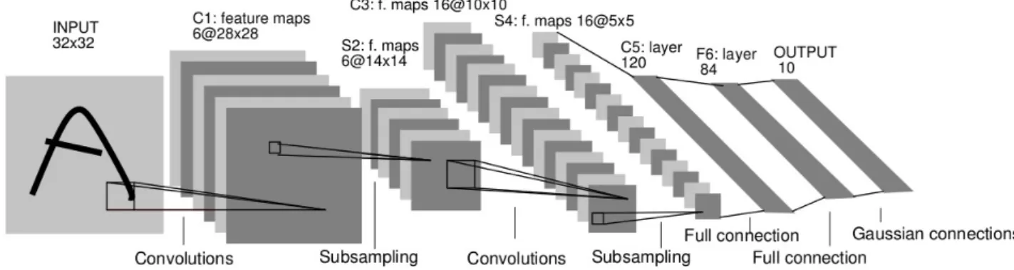
Figure 2.1 is an example of Convolutional Neural network by Le Cunn et al.

The above architecture consists of 7 layers. An image of size 32x32 pixels is fed as input to the network. Layer C1 is a convolution layer with 6 feature maps with convolution kernel of size 5x5. Layer S2 is a sub-sampling layer where each unit in S2 is connected to a 2x2 non overlapping neighbourhood of its previous convolution layer C1. The output of sub-sampling is passed through sigmoid activation function. Layer C3 is a convolutional layer with 16 feature maps using convolu-tional kernel of size 5x5. Layer S4 is a sub-sampling layer with 16 feature maps. C5 is a again a convolution layer with 120 feature maps which when convolved with 5x5 kernel will give a feature map of size 1x1, which amounts to a fully-connected layer between S4 and C5.

Figure 2.1: Architecture of LeNet-5

2.1.2

Restricted Boltzmann Machines (RBMs)

RBMs follow unsupervised learning i.e they use only inputs x(t) _{for learning and automatically}

extract meaningful features for learning. They leverage the availability of unlabelled data. An RBM is an undirected graphical model that defines a distribution over some input vector x, and models the distribution of the input vectors x using a layer of binary hidden units H.

Figure 2.2: Restricted Boltzmann Machine

The energy of RBM is defined as:

E(x, h) =−hT_{W x−c}T_x−bT_h =X j X k Wj,khjxk− X k ckxk− X j bjhj

where j,k are number of neurons in hidden and visible layers.

The probability of observing a particular configuration is given by: p(x, h) =e−E(x,h)/Z

where Z is the sum of energy of all combinations of visible and hidden, but is intractable given the combinatorial expansion of possible configuration.

In the Markov network view (given below), the notation is simply an alternative to the repre-sentation as the product of factors.

p(x, h) =e−E(x,h)/Z =e(hTW x+cTx+bTh)/Z =ehTW x/ZecTx/ZebTh/Z

Inference in RBM: Since p(x,h) is intractable due to presence of Z, we will infer using the conditional inference using either P(x|h) or p(h|x)

In RBM the conditional inference p(h|x) or p(x|h) is very easy to compute. p(h|x) =Q

j p(hj|x) Proof: = exp(h T_{W x+c}T_x+bT_h)/Z P h0∈{0,1}H exp(h0T_{W x+c}T_x+bT_h0 )/Z

As cT_{xis independent of summation in both numerator and denominator it cancels out.}

= exp(P j hjWjx+bjhj) P h0₁∈{0,1}H ... P h0_H∈{0,1}H exp(P j h0_jWijx+bjh 0 j) = _P Πjexp(hjWjx+bjhj) h0₁∈{0,1}H ... P h0_H∈{0,1}H Πjexp(P j h0_jWijx+bjh 0 j) = _P Πjexp(hjWjx+bjhj) h0₁∈{0,1}H exp(h0₁W1x+b1h 0 1)... P h0_H∈{0,1}H exp(h0_HWHx+bHh 0 H) = Πjexp(hjWjx+bjhj) Πj( P h0_j∈{0,1}H exp(h0_jWjx+bjh 0 j))

If we expand the summation which is over 0,1 in the denominator, whenh0_j is 0, it givese0_which

is 1 and whenh0_j is 1 , it gives exp(bj+Wjx)

= Πjexp(hjWjx+bjhj) Πj(1 +exp(bj+Wjx)) =Y j exp(hjWjx+bjhj) 1 +exp(bj+Wjx) = Πjp(hj |x)

Now by above theorem we have:

p(hj= 1|x) =

Y

j

exp(Wjx+bj)

1 +exp(bj+Wjx)

Multiply and divide the above equation byexp(−bj−wjx) we get,

2.1.3

Free Energy in RBM

We will see how RBM models the marginal distribution of p(x) only, i.e How RBM make certain types of inputs more likely and others less likely.

p(x) is given by, p(x) = X h∈{0,1}H p(x, h) = X h∈{0,1}H exp(−E(x, h))/Z

Lets transform the above exponential sum to linear sum

p(x) = X h∈{0,1}H exp(hTW x+cTx+bTh)/Z =exp(cTx) X h1∈{0,1} ... X hH∈{0,1} exp(hjWjx+bjhj)/Z =exp(cTx)   X h1∈{0,1} exp(h1W1x+b1h1)/Z  ...   X hH∈{0,1} exp(hHWHx+bHhH)/Z  

After expanding with the summation term,

=exp(cTx)(1 +exp(b1+w1x))...(1 +exp(bH+wHx))/Z

=exp(cTx)exp(log(1 +exp(b1+w1x)))...exp(log(1 +exp(bH+wHx))/Z

=exp(cTx+ H X j=1 log(1 +exp(bj+wjx)))/Z p(x) =exp(cTx+ H X j=1 sof tplus(bj+wjx))/Z

From the above equation we can see, p(x) is directly correlated to Network parameters namely W,b,c. Our aim is to find those set of W,b,c which can maximize p(x).

2.1.4

Energy Minimization training of RBM using Contrastive

Diver-gence

Let the problem be treated as empirical minimization problem, without Regularization. The loss function is defined in the following way [5]:

1 T X l(f(x)(t)) = 1 T X t −log(p(x(t)₎₎

where t is from 1 to T, set of all inputs. We would like to proceed by using Stochastic gradient descent ∂−logp(xt) ∂θ =Eh ∂E(x(t), h) ∂θ |x (t) −Ex,h ∂E(x, h) ∂θ

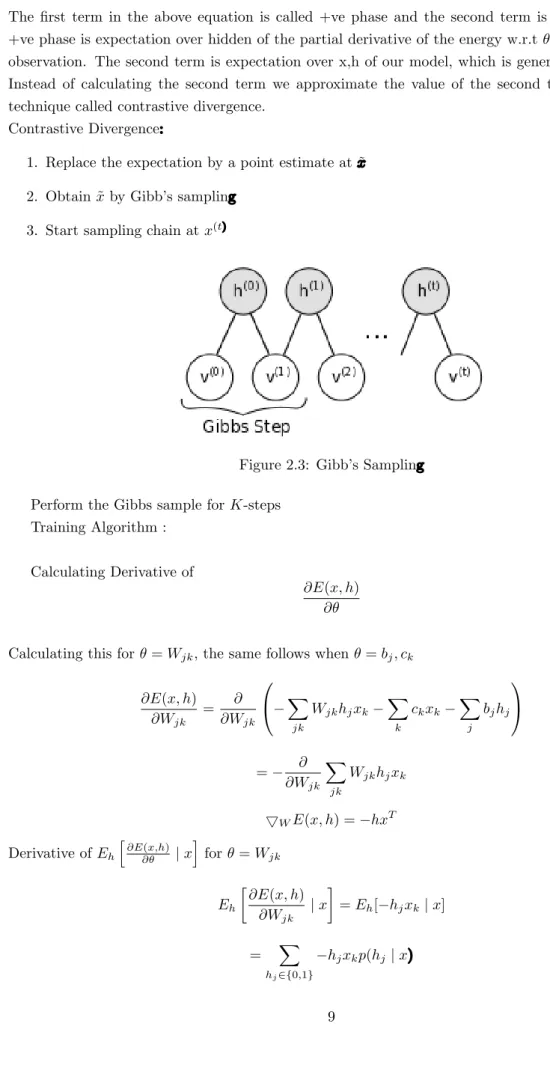
The first term in the above equation is called +ve phase and the second term is -ve phase. The +ve phase is expectation over hidden of the partial derivative of the energy w.r.tθgiven the input observation. The second term is expectation over x,h of our model, which is generally intractable. Instead of calculating the second term we approximate the value of the second term by using a technique called contrastive divergence.

Contrastive Divergence:

1. Replace the expectation by a point estimate at ˜x

2. Obtain ˜xby Gibb’s sampling

3. Start sampling chain atx(t)

Figure 2.3: Gibb’s Sampling

Perform the Gibbs sample for K-steps Training Algorithm :

Calculating Derivative of

∂E(x, h) ∂θ

Calculating this forθ=Wjk, the same follows whenθ=bj, ck

∂E(x, h) ∂Wjk = ∂ ∂Wjk  −X jk Wjkhjxk− X k ckxk− X j bjhj   =− ∂ ∂Wjk X jk Wjkhjxk 5WE(x, h) =−hxT Derivative ofEh h_∂E(x,h) ∂θ |x i forθ=Wjk Eh _{∂E(x, h)} ∂Wjk |x =Eh[−hjxk|x] = X hj∈{0,1} −hjxkp(hj|x)

=−xkp(hj = 1|x) =h(X)XT where h(X) is defined as       p(h1= 1|x) . . p(hH = 1|x)       =sigm(b+W x)

2.1.5

Update Rule

Givenx(t)_{and ˜xthe learning rule withθ=W becomes}

W ⇐W −α(5W)

W ⇐W −α(Eh[5WE(x(t), h)|x(t)]−Ex,h[5wE(x, h)])

W ⇐W−α(Eh[5WE(x(t), h)|x(t)]−Eh[5wE(˜x, h)|x]˜

W ⇐W+α(h(x(t))x(t)T −h(˜x)˜xT)

2.1.6

CD Algorithm

1. For each training examplex(t)

(i) Generate a negative sample ˜xusing K-steps of gibbs sampling, starting atx(t)

(ii) Update the parameters,

W ⇐W+α(h(x(t))x(t)T −h(˜x)˜xT) b⇐b+α(h(x(t)−h(˜x)))

c⇐c+α(x(t)−x)˜ 2. Go back to step 1,until stopping criteria

2.1.7

Gaussian Bernoulli RBM

We have seen how RBMs deal with Binary type of data. But the real world is typically con-tains all real valued data. To model real( Un bounded) valued data we use Gaussian Bernoulli RBM(GBRBM). The Energy function will get modified as

E(x, h) =−hT_{W x−c}T_x−bT_h+1

2x

T_x

The only change from normal RBM to GBRBM comes while evaluation p(x | h) which is now a Gaussian distribution with mean µ = c+WTh and identity co-variance matrix. Giving normal-ized data as input is recommended which involves subtracting each data by mean and dividing by

standard deviation.

2.1.7.1 Convolutional RBM (CRBM)

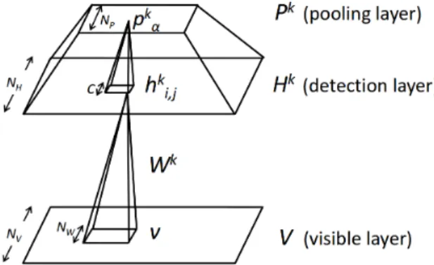
CRBM’s exploit spatially local correlation by enforcing a local connectivity pattern between neurons of adjacent layers. Different convolution operators are used to detect different types of features. The idea of CRBMs is derived from Convolutional Neural network (CNN), where there are alternating convolutional and subsampling layers. The architecture of CRBM is as below [6], CRBM consists

Figure 2.4: Convolutional Restricted Boltzmann Machine

of an input layer (V) and a hidden layer (H). Input layer is of sizeNv×Nv and the k-hidden layers

each of size Nh×Nh , each Hidden layer is associated with visible by a kernel of size Nw where

Nw=Nv−Nh+ 1 The energy for a CRBM is defined in the following way:

E(v, h) =− K X k=1 hk•( ˜Wk∗v)− K X k=1 bk X i,j hk_i,j−cX i,j vij where A•B=trATB

and∗represents convolution of anm×marray with ann×narray may result in an (m+n−1)× (m+n−1) array or an (m−n+ 1)×(m−n+ 1) array

As with standard RBMs (Section 2.1.4), we can perform block Gibbs sampling using the following conditional distributions: p(hij = 1|v) =sigm(( ˜Wk∗v)ij+bk) p(vij= 1|h) =sigm(( X k Wk∗hk)ij+c) 2.1.7.2 Gated RBM

Gated RBMs are used to model the stream of observations through the use of hidden variables which capture the dependencies between adjacent data in a stream. Given below is the architecture of a Gated RBM [7]. A Gated RBM consists of an input layer X, an output layer Y and a hidden layer H. The dependencies among these three layers are modelled by using a three dimensional tensor Wijk

Figure 2.5: Gated RBM

The energy function that is used to capture the dependencies between input, output and hidden is given byE(y, h;x) =−P

ijkWijkxiyjhk

The joint distributionp(h, y|x) is defined fromE(y, h;x) as

p(h, y|x) = 1 Z(x)exp(−E(y, h;x)) where Z(x) =X y,h exp(−E(y, h;x))

The distribution over output given input is obtained by marginalizing over hidden as: p(y |x) = P

hp(y, h |x) In gated RBM, only the hidden and output units are inferred for learning, and the

inputs are always kept constant. The sampling of hidden units is done using the following expression:

p(hk = 1|x, y) =

1 1 +exp(−P

ijWijkxiyj)

Similarly the output units are sampled using:

p(yj = 1|x, h) =

1 1 +exp(−P

ikWijkxihk)

Learning occurs in Gated RBM by maximizing the conditional log likelihood L, where,

L= 1 N

X

α

logp(yα|xα)

for all N training samples (xα_{, y}α_{) The gradient of L is given by difference of two expectations as}

below: ∂L ∂W = X α _∂E(yα_{, h;x}α₎ ∂W h − _{∂E(y, h;x}α₎ ∂W y,h

2.1.7.3 Factored RBM

A factored RBM is simply an extension of Gated RBM. Gated RBMs are used to model the pair-wise interactions between input and output using a three-dimensional tensorWijk. But this tensor

has too many parameters to be learned. Hence, the Wijk in a Gated RBM can be approximated

by factoringWijk asWif, Wjf, Wkf where f is the number of factors [8].This factoring reduces the

number of parameters fromO(n3_{) toO(n}2_{) if the size of f is comparable to other units. Given below}

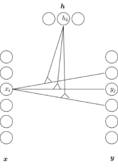
is the architecture of a Factored RBM [9],

Figure 2.6: Factored RBM : The triangle in the middle represents factors

The energy equation of Factored RBM becomes : −E(v, h) =P

f(

P

iviWif)(PjvjWjf)(PkhkWkf)

The learning happens just like in gated RBM by maximizing the log likelihood, with gradient cal-culated as ∂L ∂w =h ∂E ∂wih− h ∂E ∂wiy,h

2.2

Related Work: Deep Learning for Action Recognition

This section explains various methods that are used in deep learning methods for action recognition in videos. We will discuss two main approaches, viz. 3D Convolutional Neural Networks (CNNs) approach and Convolutional Gated RBM (CGRBM) approach for action recognition. There are many other approaches proposed for the action recognition problem that are not based on deep learning, but they are not discussed here as our focus is on the possibility of infusing the concept of temporal coherence in deep learning architectures.

2.2.1

3D CNN for Action Recognition

2D CNNs are capable of only modelling the spatial features in a given input data. But a video comprises of temporal information which plays a crucial role in detecting actions in a video. To model this, 2D CNNs are extended as 3D CNNs with temporal data as the third dimension.The figure below explains how 3D convolution is performed. To summarize, 3D convolution is performed

Figure 2.7: 3D convolution

by using a convolutional kernel of three dimensions, which convolve consecutive images from a given video. The value at position (x, y, z) on thejthfeature map in theithlayer is defined as:

vxyz_ij =tanh(bij+ X m Pi−1 X p=0 Qi−1 X q=0 Ri−1 X r=0 w_ijmpqrv₍(x_i−+₁₎p)(_my+q)(z+r))

where Ri is the size of the 3D kernel along the temporal dimension. Figure 2.8 shows an example

of 3D CNN [10]

Figure 2.8: 3D convolution

The input to 3D CNN is 7 images of size 60x40, which are hardwired to give 33 images of same size in Layer H1. A 3D kernel of shape 7x7x3 is applied on all these images resulting in 23*2@54x43 images in layer named C2. A kernel of size 7x7 is then applied on each image and by considering

three images in the temporal direction. The layer C2 undergoes subsampling, resulting in reducing the size of image by half in both axis resulting in 23*2@27x17 in layer S3. This alternating of 3D convolution and subsampling continues for layers C4 and S5, and a 2D convolution is finally applied between layers S5 and C6 resulting in scalar quantities which are fully connected to output neurons. The number of output neurons is equal to the number of actions in our data set used. This 3D CNN gave state-of-the-art performance on one of the most difficult data sets for action recognition, viz. the TRECVID dataset.

2.2.2

Convolutional Gated RBM (CGRBM) for Action Recognition

This approach in deep learning is a combination of RBMs and 3D CNNs for action recognition in videos. As the gated RBM suffers from the problem of learning too many parameters i.e ofO(n3), this approach uses the advantage of weight-sharing through convolution. The architecture of a Con-volutional Gated RBM is shown in Figure 2.2.2. The Gated Factored RBM is similar to the Gated

RBM, except for the change that the three way interaction between input, output and hidden are performed using convolution operations. The input and output images are of size Nx×Nx and

Ny×Ny respectively. The number of feature maps are K, resulting inKNz×Nz feature maps.

The energy of a CGRBM is defined as [11]:

E(y, z;x) =− K X k=1 Nz X m,n=1 Ny w X r,s=1 zkm,nγ(x)kr,s,m,nym+r−1,n+s−1− K X k=1 bk Nz X m,n=1 zkm,n−c Ny X i,j=1 yi,j The filter γ(x)k r,s,m,nym+r−1,n+s−1 = PN x w u,vW k

r,s,u,vxm+u−1,n+v−1 The probability of hidden units,

output being active is given by:

p(zk_m,n= 1|x, y) =sigm( Ny w X r,s=1 γ(x)k_r,s,m,nym+r−1,n+s−1) +bk

p(yi,j= 1|x, h) =sigm( K X k=1 N_wy X r,s=1 ˜ γ(x)r0_,s0_{,i+r−1,j+s−1}˜z_ik_{+r−1,j+s−1}+c)

wherer0=Ny

w−r+1 ands0=Nwy−s+1 and also flips the matrix in horizontal and vertical direction.

In the next chapter, we describe the proposed method to incorporate temporal coherence in videos, building on top of the Convolutional Gated RBM.

Chapter 3

Temporal Coherence in

Energy-Based Deep Models:

Proposed Methodology

3.1

Modelling temporal sequences of videos

The CGRBM models the joint energy of two input images. In a given video, two consecutive frames in a video will be very similar. We can use this property to model the energy curve modeled by the CGRBM in such a way that the similar images will be at lower energy states and we intentionally pull up the joint energy for dissimilar images.

The overall loss function for CGRBM is:

L(θ) =−1

NE(y, z;x)

and the update rule is defined as:

θ=θ−λ∂L(θ, x, y, z) ∂θ , whereλis the learning rate.

Our proposed approach works in the following manner. When the CRBM is given inputs as current dataX and past dataY, where X,y are two input images, the CGRBM models the joint energy of these two images and updates its weights so as to reduce its energy. To leverage the property of temporal coherence in modelling the joint energy of consecutive images in CGRBM, the loss function is redefined as:

Lcoh(x, y, θ) =

  

argminθE(y, z;x), similar

argmaxθE(y, z;x), otherwise

be-low.

Data: Image pairs (Xi, Yi, typei), i=1..n

Result: Set of Weights which minimizes the joint energy for Consecutive image pairs and maximizes for other

Initialize Weights and biases of the network to Uniform random numbers; whileepochs do

read an image pairxi, yi;

if typei==’similar’ then

Do Contrastive Divergence to decrease the joint energy of E(y,z;x); else

Do Contrastive Divergence to increase the joint energy of E(y,z;x); end

end

Algorithm 1: Proposed Learning Algorithm for Deep Energy Based Models with Temporal Co-herence

We use Gibbs sampling to perform Contrastive Divergence to leverage the property of conditional independence of nodes in a given layer.

Data: Image pairxi, yi, typei

Result: Updated Weights of the network

Sample the hidden units(Z) conditional on Past(X),Data(Y);

Sample the data units(Y) conditional on Hidden,Past(X); /* End of positive phase */

Compute the positive grads of W,hidbias,visbias; while number of Gibb’s iterations do

Sample the hidden units(Z) conditional on Past(X),Data(Y);

Sample the data units(Y) conditional on Hidden(Z) ; /* End of Negative Phase */

end

Compute the negative grads of W,hidbias,visbias;

if typei==’similar’ then

gradW=posgradW-neggradW; else

gradW=-posgradW+neggradW; end

Algorithm 2: Contrastive Divergence Algorithm for the Proposed Method

The proposed method above framework can also be generalized to other coherence settings, beyond temporal coherence. The same framework can be used to any type of data with similarity defined as per the data. For video data, we have taken past frames as temporally coherent, and frames from other actions as non-coherent, but this can be easily changed as evident.

Chapter 4

Experimental Results

4.1

Experimental Setup

We had experimented on the following setup of CGRBM. While modelling the NORB dataset, the input size is resized to 22x22 and filters of size 9x9x9x9 are used with number of feature maps as 1. The temporally coherent frame for NORB is defined as an image that is rotated 20 degree. In the initial epochs the ratio is similar to dis similar frames is kept at 2:1 and after few epochs its kept at 1:1.

For KTH the input size of an image is kept at 80x60 and the number of filters are kept at 9x9x9x9. A subsampling of 4x4 is used for probabilistic max-pooling. The ratio of similar to dis similar is kept at 9:1. A total of 76 video clips from each action is given as training set and the rest 24 from each action are given as test set.

4.2

Experimental Results on NORB Data set

The modified algorithm is applied on small NORB data set [12].The database consists of objects from five different categories: animals, human figures, airplanes, trucks, and cars. These objects are viewed under different lightening, elevations and Azimuth settings. We have considered objects differing by Azimuth and trained a convolutional Gated RBM and the CGRBM learns the transfor-mations between the images just like optical flow.

The quiver plots of the CGRBM transformations looks similar to Optical flow between the two images that differ by certain Azimuth. A sample car objects are taken and given to CRBM.

Figure 4.2 is the transformation the CGRBM has learnt,

The norb data set size is down sampled to 32x32 size and a filter of size 9x9 is used to do convolution operations. A pooling of size 2x2 is used at probabilistic max pooling. The ratio of dis similar to similar is given as 1:3. If the ration is given as 1:1 , there is a danger of disturbing the entire energy curve with many ridges and valleys to the energy curve.

The ratio can be increased after few epochs of training as the shape of the curve stabilizes after few iterations

Figure 4.1: Input to CGRBM

Figure 4.2: Transformations learnt by CGRBM

4.3

Experimental Results on KTH Data set

KTH is an Human Action Recognition data set [13]. It contains action of six different types per-formed by 25 subjects in four scenarios.

The following is the confusion matrix for KTH dataset. The ratio of train to test is 3:1

Action Walking Jogging Running Boxing Waving Clapping

Walking 21 0 1 1 0 2 Jogging 0 20 4 0 0 0 Running 0 3 21 0 0 0 Boxing 0 0 0 21 2 1 Waving 0 0 0 1 21 2 Clapping 0 0 0 1 3 20

An accuracy of 85.52% is achieved using the KTH dataset.

The CGRBM is trained on KTH data set and the following are the hidden inferences obtained after training the CGRBM for one full epoch.

Figure 4.3: Hidden Inferences of action walking

Figure 4.4: Hidden Inferences of action boxing

Chapter 5

Conclusions and Future Work

5.1

Where does our approach work and why?

Our approach of modified learning algorithm works for data which has a temporal coherence embed-ded in it. Several types of data like stock market prices, weather ratings,speech data,video data, etc where the current instance of data is dependent on the previous instances can be modelled by our approach. Our approach would be of great interest to those type of data that has temporal coherence embedded into it as the CGRBM models the transformation in a given data as the learning itself is happening considering the previous data into account.

5.2

Directions for Future Work

This work can be extended to include more past data while modelling the current instance of data. This can help us to model the data much better.

5.3

Conclusions

A novel idea of inclusion of similar and dissimilar data during training is introduced and the learning algorithm is modified so that it could better model the Joint energy curve. The proposed learning approach is applied on NORB data set and KTH data set and the results are studied and analysed.

References

[1] L. Deng. A tutorial survey of architectures, algorithms, and applications for deep learning.

APSIPA Transactions on Signal and Information Processing 3.

[2] Y. Lecun, S. Chopra, R. Hadsell, F. J. Huang, G. Bakir, T. Hofman, B. Schlkopf, A. Smola, and B. T. (eds. A tutorial on energy-based learning. In Predicting Structured Data. MIT Press, 2006 .

[3] J. Aggarwal and M. Ryoo. Human Activity Analysis: A Review. ACM Comput. Surv. 43, (2011) 16:1–16:43.

[4] Y. LeCun, L. Bottou, Y. Bengio, and P. Haffner. Gradient-Based Learning Applied to Document Recognition. In Proceedings of the IEEE, volume 86. 1998 2278–2324.

[5] G. E. Hinton. Training Products of Experts by Minimizing Contrastive Divergence. Neural

Computation 14, (2002) 1771–1800.

[6] H. Lee, R. Grosse, R. Ranganath, and A. Y. Ng. Convolutional Deep Belief Networks for Scalable Unsupervised Learning of Hierarchical Representations. In Proceedings of the 26th International Conference on Machine Learning. 2009 609–616.

[7] R. Memisevic and G. Hinton. Unsupervised Learning of Image Transformations. In Proceedings of IEEE Conference on Computer Vision and Pattern Recognition. 2007 .

[8] M. A. Ranzato, A. Krizhevsky, and G. E. Hinton. Factored 3-Way Restricted Boltzmann Machines For Modeling Natural Images 2010.

[9] M. Ranzato, A. Krizhevsky, and G. E. Hinton. Factored 3-Way Restricted Boltzmann Machines For Modeling Natural Images. Journal of Machine Learning Research - Proceedings Track 9, (2010) 621–628.

[10] S. Ji, W. Xu, M. Yang, and K. Yu. 3D Convolutional Neural Networks for Human Action Recognition. IEEE Trans. Pattern Anal. Mach. Intell.35, (2013) 221–231.

[11] G. W. Taylor, R. Fergus, Y. Lecun, and C. Bregler. Convolutional Learning of Spatio-temporal Features.

[12] Y. LeCun, F. J. Huang, and L. Bottou. Learning Methods for Generic Object Recognition with Invariance to Pose and Lighting. In Proceedings of the 2004 IEEE Computer Society Conference on Computer Vision and Pattern Recognition, CVPR’04. IEEE Computer Society, Washington, DC, USA, 2004 97–104.

[13] C. Schuldt, I. Laptev, and B. Caputo. Recognizing Human Actions: A Local SVM Approach. In Proceedings of the Pattern Recognition, 17th International Conference on (ICPR’04) Volume 3 - Volume 03, ICPR ’04. IEEE Computer Society, Washington, DC, USA, 2004 32–36.