ISSN 0956-8549-632
The Lifecycle of the Financial Sector
and Other Speculative Industries
By
Bruno Biais
Jean-Charles Rochet
Paul Woolley
THE PAUL WOOLLEY CENTRE
WORKING PAPER SERIES NO 4
FMG DISCUSSION PAPER 632
DISCUSSION PAPER SERIES
April 2009
Bruno Biais is research professor of economics and finance at the Toulouse School of
Economics (IDEI, CNRS). He is currently editor of the Review of Economic Studies.
Bruno Biais has been scientific adviser to Euronext, EuroMTS, the London Investment
Banking Association and the New York Stock Exchange. He held the Deutsche Bank
visiting chair of finance at Oxford University, was Wim Duisenberg Fellow at the
European Central Bank, and gave the Rotman Distinguished Lectures at the University
of Toronto. Jean - Charles Rochet holds a Ph.D in Mathematical Economics from Paris
– Dauphine University . He has taught in Paris, France (Dauphine University, ENSAE
and Ecole Polytechnique) and London, U.K. ( B.P. visiting professor, London School of
Economics, 2001-02). He is a member of the Institut Universitaire de France and a
Fellow of the Econometric Society since 1995. He has also been council member of
European Economic Association, and associate editor of Econometrica . He is currently
Professor of Economics at the Toulouse School of Economics and Research Director at
Institut D’Economie Industrielle. Paul Woolley’s career has spanned the private sector,
academia and policy-oriented institutions. He has worked at the International Monetary
Fund in Washington and as a director of the merchant bank Baring Brothers. For the
past 20 years he has run the European arm of GMO, the global fund management
business based in Boston, US. Dr Woolley funded The Paul Woolley Centre for the
Study of Capital Market Dysfunctionality. He is chairman of the Advisory Board for the
Centre and is a full time member of the research team. Any opinions expressed here are
those of the authors and not necessarily those of the FMG. The research findings
reported in this paper are the result of the independent research of the authors and do
The Lifecycle of the Financial Sector and Other Speculative
Industries
Bruno Biais1, Jean—Charles Rochet2 and Paul Woolley3
April 24, 2009
This research was conducted within the Paul Woolley Research Initiative on Capital Market
Dys-functionalities at IDEI, Toulouse. Many thanks to participants at thefirst conference of the Centre for
the Study of Capital Market Dysfunctionality at the London School of Economics, June 2008, as well
as seminar participants in Frankfurt University and Amsterdam University, especially Arnoud Boot,
Markus Brunnermeier, Catherine Casamatta, Guido Friebel, Alex Gümbel, Enrico Perotti, Ludovic
Phalippou and Guillaume Plantin.
1Toulouse School of Economics (CNRS-GREMAQ & PWRI-IDEI) 2
Toulouse School of Economics (CNRS-GREMAQ & PWRI-IDEI)
3
Abstract
Speculative industries exploit novel technologies subject to two risks. First, there is uncertainty
about the fundamental value of the innovation: is it strong or fragile? Second, it is difficult to monitor
managers, which creates moral hazard. Because of moral hazard, managers earn agency rents in
equilibrium. As time goes by and profits are observed, beliefs about the industry are rationally
updated. If the industry is strong, confidence builds up. Initially this spurs growth. But increasingly
confident managers end up requesting very large rents, which curb the growth of the speculative
sector. If rents become too high, investors may give up on incentives, and risk and failure rates rise.
Furthermore, if the innovation is fragile, eventually there is a crisis, and the industry shrinks. Our
model thus captures important stylized facts of the financial innovation wave which took place at the
beginning of this century.
1
Introduction
Technical innovations can generate booms. Such developments are risky when the fundamental
prof-itability of the innovation is unknown. Furthermore, the actions and performance of managers are
particularly difficult to monitor in innovative industries, with which final investors are not familiar.
This creates a moral hazard problem. As the industry spurred by the innovation grows, its potential
value develops, but its riskiness and the agency problem can worsen. And if the risk eventually
ma-terializes, crises can take place. The goal of this paper is to model the equilibrium dynamics of such
speculative industries.
A prominent example is the development of thefinancial sector at the beginning of this century.
Technological advances in information technologies, combined with market liberalization, spurred
many innovations, both in terms of techniques, e.g., securitization, and in terms of strategies and
institutions, e.g., hedge funds and private equity funds. Innovation generated remarkable growth, in
terms of capital invested, attraction of skilled workforce and market valuation. Significant profits
were generated. Nevertheless, doubts remained. Were the financial innovations valuable enough to
justify the allocation of so muchfinancial and human capital? Did the fund managers and investment
bankers really exert the right amount of effort and did they make the right decisions to ensure that
investment would be valuable? Were the level of compensation tofinancial managers and their growth
sustainable? Or would rents eventually absorb all the value creation in the industry?
We investigate these issues in the context of an agency model with rational expectations and
learning. There are two sectors: the traditional one and the innovative one, which we refer to as
the speculative industry. There is a continuum of competitive managers, who choose to work in the
speculative industry if the wage it offers exceeds their compensation in the traditional sector. For
simplicity we assume the traditional sector is well known, so that agency problems and uncertainty
are not an issue there. Thus managers working in that sector receive wages equal to their known
and in terms of challenges.
• First, there is uncertainty. The speculative sector can be strong and potentially very profitable. Alternatively it can be fragile and exposed to the risk of a crisis. Observing the dynamics of
realized profits in the speculative sector, agents conduct Bayesian learning about the strength
of that industry.
• Second, there is asymmetric information. In the speculative sector it is not easy to monitor how managers use the resources they have been entrusted with. The managers may be tempted
to use these resources in ways that are not optimal for the final investors. Thus, this sector is
plagued with moral hazard, which we model in the line of Holmstrom and Tirole (1997): when
managers fail to exert effort, they earn private benefits from shirking, but the probability of
success is lowered.
Our key assumption is that the nature of the moral hazard problem is related to the fundamental
value of the innovation. We assume that if the innovation is strong managerial shirking does not
reduce very much the probability of success, while if the innovation is fragile shirking significantly
increases the risk of failure. To motivate this assumption consider the example of the innovation wave
brought about by such techniques as securitization and credit default swaps. The initial uncertainty
is about the extent to which these innovations would enable banks to reduce their exposure to the
risk of defaults. A strong innovation is very effective at shedding this risk. A fragile one leaves banks
exposed to high risks. In this context, consider the consequences of effort. If bankers exert high effort,
they screen out most bad projects. In that case, whether the innovation is strong or fragile, they
are exposed to limited default risk. In contrast, if banks shirk and fail to scrutinize loan applicants
carefully, they remain relatively safe when the innovation is strong, but are exposed to high default
risk when it is fragile.
Ironically, our assumption that the adverse consequence of shirking is greater when the innovation
when the adverse consequences of shirking on success are limited, shirking is attractive for the manager.
Hence agency rents are higher. In that context, our model yields the following equilibrium dynamics:
• Boom: In the early phase of the innovation wave, if there is no crisis, confidence builds up. Correspondingly the speculative sector attracts an increasing fraction of capital and labor.
• Choking: If performance continues, managers become very confident. Hence they demand large rents. These limit the net returns left to investors and slow down the growth of the speculative
sector.
• Risk—Taking: At some point, the rents demanded by the managers become so high that in-vestors give up on incentives. Consequently, managers screen projects lesss carefully, and default
rates go up.
• Bust: At any point, if the industry is fragile, there can be a crisis.4 When it occurs, agents revise downwards their expectations about the profitability of that sector. Consequently, investment,
wages and employment in the speculative industry drop.
Thus, our model is in line with some of the major stylized facts of the financial innovation wave
of the early 2000s and its eventual bust:
• Uncertainty, learning and growth: Before the crisis, some analysts claimed that securiti-zation and risk management techniques had very significantly reduced (if not eliminated) the
macro—risk associated with the financial sector. For example, A. Greenspan said in a speech
delivered in 2005: “As is generally acknowledged, the development of credit derivatives has
contributed to the stability of the banking system by allowing banks, especially the largest
sys-tematically important banks, to measure and manage their credit risk more effectively”. In the
4
While the Boom, Choking and Risk—Taking regimes arise both for solid and for fragile innovations, crises take place only when the innovation is fragile.
language of our model, this corresponds to the belief that the speculative industry was strong.
As in our model, such optimistic beliefs were motivated by a series of years with high profits
and no largefinancial distress. As in our equilibrium, these developments were accompanied by
an increase in the size of the financial sector.
• Managers’ rents and investors’ net returns: Our theoretical analysis implies that dur-ing the successful stages of financial innovation waves, managers operating in the speculative
industry earn increasing rents. This is consistent with the empirical results of Philippon and
Reshef (2008). Theyfind that, during the recentfinancial innovation wave, the compensation of
managers in thefinancial sector increased relative to other sectors. Furthermore, they estimate
that part of that increase reflected rents. Our model also implies that, as long as there is no
crisis, the relationship between the amount of money invested in the speculative sector and its
past performance should be inverse U—shaped, which is constisent with the empirical results of
Ramadorai (2008). The economic intuition we provide for this fact is that, initially, the increase
in confidence due to good records attracts funds, while later confidence inflates managers’ rents,
which undermine net returns to investors.
Our analysis on the role of uncertainty and learning in booms and crashes is in line with the
contributions of Zeira (1987, 1999), Rob (1991), Pastor and Veronesi (2006), and Barbarino and
Jovanovic (2007). These papers offer rational expectations models where, in presence of uncertainty
and learning, an industry can develop as long as good news are observed and then crash with bad
news. Zeira (1999) shows that his theoretical model applies to the booms and crashes of 1929 and
1987. Pastor and Veronesi (2006), and Barbarino and Jovanovic (2007) show that their models offer
insights into the boom and crash of the telecommunications and internet sector in the late 1990s.
One contribution of our analysis relative to these papers is to introduce moral hazard and study
how it affects the dynamics of the innovative industry.5 This enables us to generate new results relative
5
to the previous literature. We study the interaction between moral hazard and learning. We show how
rents arise in equilibrium. We explain how the evolution of these rents affects the dynamics of the
division of the value between managers and investors. We also show how moral—hazard can lead to
excessive risk—taking at a systemic level.
Symmetrically, our paper also contributes to the literature by showing how the moral hazard
problems arising in innovative industries are altered by learning. Thus, our model is in the line of
Bergemann and Hege (1998). Yet the focus of the two papers is quite different. Bergemann and Hege
(1998) offer an insightful analysis of long term Venture Capital contracts which is beyond the scope of
our one—period contracting framework. But, while Bergemann and Hege (2008) study the interaction
between two players only, we consider populations of investors and managers and characterize the
lifecycle of the speculative industry, the allocation of human and physical capital to the innovative
and traditional sectors, and the evolution of rents and risk—taking.6
Our work is also in line with Philippon (2008) who analyzes the interaction between thefinancial
and non—financial sectors. But, in his model, agency problems plague the real sector, and monitoring by
financial intermediaries mitigates the moral hazard problem facing manufacturingfirms by monitoring them. In contrast, our analysis assumes moral hazard in the speculative industry. Finally, our analysis
is also related to Lorenzoni (2008), who offers a model of credit booms with agency problems and
aggregate shocks, where credit expansion can be followed by contractions. But his focus on pecuniary
externalities differs from our focus on the interaction between learning and incentives.
The next section presents our model. Section 3 presents the benchmark case where effort is
observable. It shows how booms and crashes can arise, because of uncertainty and learning, without
emphasis on moral hazard makes our model particularly relevant for the recent evolution of thefinancial industry where agency problems were key.
6
There is another, more technical difference, relative to the nature of the learning process in the two papers. In Bergemann and Hege (1998) there is learning about the probability of rare successes, so that no news is bad news. In contrast, in our model, there is learning about the probability of rare crises, so that no news is good news. This generates different learning dynamics.
moral hazard. Section 4 turns to the case where managerial effort is unobservable. It shows how
moral hazard interacts with learning and gives rise to choking and risk—taking. Section 5 discusses
the implications of our analysis and confronts them with empirical evidence on the financial sector.
Section 6 concludes and briefly discusses some policy implications. Proofs omitted in the text are in
the appendix.
2
The model
2.1
Agents and goods
Consider an infinite horizon economy, operating in discrete time at periodst= 1,2, ... There is a mass one continuum of competitive managers and a mass one continuum of investors. All players are risk
neutral. The managers have limited liability and no initial wealth. At the beginning of each period,
each investor is endowed with one unit of nonstorable investment good. At the end of each period,
all agents consume the consumption good, produced, as explained below, by labor and capital. For
simplicity, we focus on the simplest possible case, where managers and investors live only one period,
and contracts are for one period.7 Yet, the model is dynamic, to the extent that agents progressively
learn about the state of the economy. Thus, the link between generations runs through the evolution
of beliefs.
2.2
The two sectors
2.2.1 Managers and investors
Managers and investors are heterogeneous. Their types are denoted by ν and ρ respectively. The types of the manager are distributed over [0,¯ν]. Their cumulative distribution function is denoted by G. The types of the investors are distributed over[0,¯ρ]. Their cumulative distribution function is
7When palyers interact for several periods, shirking can crete a wedge between the beliefs of investors and managers.
denoted by F.
There are two productive sectors, the traditional sector and the speculative one. Managers and
investors choose in which sector to operate. For simplicity we asssume that, in the traditional sector,
agents generate output equal to their type. Thus, ν is the productivity of the managers in the traditional sector. When the type ν manager operates in the traditional sector, he obtains, at the end of the period, ν units of the consumption good. Similarly, when investor ρ allocates her unit endowment of investment good to the traditional sector, she obtains ρunits of the consumption good at the end of the period.
The innovative technology requires one unit of investment as well as managerial effort. Capital is
provided by the investors, who are endowed with the investment good at the beginning of the period.
Managers are hired by investors.
2.2.2 Uncertainty
There is uncertainty about the speculative industry. Consider for example the securitization of
sub-prime mortgages. It was not initially clear whether or not structured finance techniques could reduce
exposure to defaults and improve the allocation of risk without generating perverse effects. Analogous
securitization techniques had worked well previously for other types of assets, such as credit card
re-ceivables. But this newfinancial innovation wave had novel and yet untested characteristics, and there
was uncertainty about how it could perform in the long run. While it could not have obviously been
predicted that ex ante, it eventually turned out that the new securitization process involved intrinsic
flaws, due to the interdependence between financial institutions, counterparty risk and its interaction with the real estate bubble.
We model this uncertainty by assuming that the speculative technology can either be strong, which
is denoted byθ= 1, or fragile, which is denoted byθ= 0. If the industry is strong, it is immune from crises. But, if the industry is fragile, at each period, with probability 1−p, it can be hit by a crisis. In that case, all projects in the speculative sector generate 0 output. Thus, fragility implies that the
industry is exposed to the risk of a large crisis annihilating its profits.
2.2.3 Moral hazard
When there is no crisis, speculative sectorfirms generateRor 0. The distribution of output in that case depends on the effort of the managers. Managerial effort leads to an improvement in the distribution
of output in the sense of first order stochastic dominance. This can be interpreted as an increase in
the probability of success, e.g., in high—tech industries the manager can exert effort to increase the
probability that a new patent will be obtained and a new product or service will be commercialized.
Effort can also be interpreted in terms of risk prevention, e.g., in the financial sector managers can
exert effort to screen investment opportunities, and avoid those with a large risk of default.
When there is no crisis, if a manager exerts effort, outputRis generated for sure. But if he exerts no effort, there is a risk that output will be 0. When the industry is strong, the probability of default
under shirking, denoted by ∆, is relatively small, but when the industry is fragile, the default rate
under shirking can be is higher: with probabilityλit is the same as for the solid industry (i.e. ∆), and with probability 1−λ it is ∆¯ >∆. The expected default rate under shirking in the fragile industry (λ∆+ (1−λ) ¯∆) is denoted by ∆ˆ.
To illustrate this consider the case of securitization of loans. Our assumption means that when the
structuredfinance techniques is fragile (say in the case of subprime mortgages), there is a probability
1−λthat shirking (i.e. not exerting due diligence in the screening and monitoring of borrowers) will result in higher default rates than for the solid industry, even in the absence of a crisis. By contrast if
the industry is strong (as the securitization of credit card receivables) shirking is less damaging. Thus,
when the industry is fragile not only is it exposed to crises (with probability1−p there is a crisis and all firms obtain 0 return), but also it is exposed to smaller micro—shocks (with probability 1−λthe adverse consequences of shirking are greater than they would have been for the strong industry).
obtains a private benefit from shirking, denoted byB. Hence there is a moral hazard problem.8 The investor is the principal and the manager the agent. The extensive form of the game within a period
is represented in Figure 1.
We now introduce our two key maintained assumptions. First, we assume
A1 :p∆ˆ >∆,
which means that the expected negative consequences of shirking on output are greater when the
industry is fragile than when it is solid.9 In other words, strong industries are more robust to shirking
than fragile ones. Second, we assume
A2 :∆R > B.
which, jointly with A1 implies that effort is socially optimal, and would take place in the first best,
i.e.,
(πt+ (1−πt)p)R >(πt(1−∆) + (1−πt)[1−∆ˆ]p)R+B,∀πt.
2.3
Learning
All the agents in the economy observe all returns realizations, and use these to conduct rational
Bayesian learning about θ. At the first period, agents start with the prior probability, π1, that
θ = 1.For t > 1, denote by πt the updated probability that the speculative industry is strong, given the returns realized in the speculative sector at times{1, ...t−1}. By the law of large numbers, aggregate default rates may reveal a lot of information. For example, Figure 1 shows that an aggregate
default rate of either ∆¯ (large number of individual losses) or 1 (systemic crisis) can only come from a fragile industry. Thus the fragility of an industry is detected for sure (andπtgoes to0)as soon as the
8As in Holmstrom and Tirole (1994) we cast the problem in terms of private benefits foregone by the manager when
exerting effort. One could equivalently consider a model without private benefits but where effort would be costly.
average default rate strictly exceeds ∆.10 Until this date, πt remains strictly between 0 and 1. Thus if all projects succeed at date t, it implies that managers have exerted effort and the probability that the industry is strong has to be revised upward:
πt=
πt−1
πt−1+p(1−πt−1)
> πt−1. (1)
By contrast if the default rate is ∆,this shows that managers have shirked. Yet, the probability that the industry is strong increases even further:
πt=
πt−1
πt−1+λp(1−πt−1)
> πt−1, (2)
since, in spite of shirking, the aggregate default rate has been limited. This is because,when the
industry is fragile, shirking implies a positive probability of default rates in excess of ∆.11
Thus, as long as the average return offirms operating in the speculative sector is sufficiently good,
beliefs about θimprove. But, when it is too low, confidence melts down and πt suddenly falls down to 0.
2.4
Contracts
At time t, newly born investors and managers interact for one period. We assume however that they have access to the complete performance history of the industry, which implies that they share the
updated belief πt.
First consider the case where the contract stipulates that managers are to exert effort. If there
is a crisis all projects fail, while otherwise all projects should succeed, and obtain return R. If the output of the project run by manageriis equal to 0, while others succeeded, it must be that manager
1 0If a crisis could also occur whenθ = 1, while remaining less likely than for θ= 0, the learning process would be
smoother. But it would have the same major qualitative feature, i.e.,πtwould increase after good returns and decrease
after bad returns.
1 1
If this property was satisfied with certainty (ifλwas equal to0) then the fragility of the industry would be inferred as soon as the managers would shirk, since it would lead to an aggregate default rate of ∆¯ incompatible with a strong innovation.
i shirked. It is optimal to set his compensation to 0 in that case. Also, it is weakly optimal to set managerial compensation to 0 when there is a crisis and all firms obtain 0 output.
Second, consider the case where the contract stipulates managers are not to exert effort. In that
case, only the expected compensation of managers matter, not its allocation across states. Hence, it
is weakly optimal to compensate the manager only when the output of his firm isR.
Accordingly, we consider contracts where managers are compensated only when theirfirm generates
output R. We denote the value of this compensation at time t by mt, which could be interpreted as the bonus, received by managers if and only if they succeed.
3
Equilibrium when e
ff
ort is observable
Consider first the benchmark case where effort is observable. In that case, since effort is efficient,
managers are simply instructed to exert it, and their compensation is set to clear the labour market.
At time t, the expected output of firms operating in the speculative sector is:
St= [πt+ (1−πt)p]R, (3) and the expected compensation of the managers is:
Mt= [πt+ (1−πt)p]mt,
while investors obtainSt−Mt in expectation. Managers with opportunities in the traditional sector belowMtprefer to operate in the speculative sector. Hence, the supply of managers for that sector is:
G(Mt). (4)
Investors whose return opportunities in the traditional sector are belowSt−Mtprefer to invest in the speculative one, and thus need to hire a manager. Hence, the demand for managers in the speculative
sector is:
Equating (4) and (5) the labour market—clearing condition is:
G(Mt) =F(St−Mt). (6) The supply of managers is continuous and increases fromG(0) = 0toG(¯ν) = 1, while the demand for managers is continuous and decreases from F(St) > 0 to 0. Consequently there exists a unique solution Mt∗ to (6). In our simple model a natural measure of the size of the speculative sector is the number of managers, or equivalently the number of firms operating in that sector. Based on the
discussion above, we state our first proposition (illustrated in Figure 2, Panel A):
Proposition 1: When effort is observable, the equilibrium expected compensation of managers in the speculative sector is Mt∗ (the solution of (6)) and the size of that sector is: G(Mt∗).
Suppose that, up tot−1, there has been no crisis and the updated probability that the industry is strong is πt. If during period t there is no crisis, then investors become more optimistic and the updated probability that the industry is strong goes up to πt+1 > πt. Thus expected output in the speculative sector increases and the demand curve (5) goes up, while the supply curve (4) stays
constant. Consequently, the equilibrium compensation of managers in period t+ 1 isMt∗+1> Mt∗. In contrast, after a crisis, the updated probability that the industry is strong goes down to 0 and the
expected output in that industry goes down to pR. Consequently the size of the speculative sector shrinks. These remarks are summarized in the following corollary:
Corollary 1: When effort is observable, as long as there is no crisis the size of the speculative sector goes up, along with the expected compensation of managers employed in that sector. When there is a crisis, the size of the speculative sector and the equilibrium expected compensation of managers suddenly drops.
4
Equilibrium under moral hazard
4.1
Incentive compatibility
When effort is not observable but requested, we must impose the incentive compatibility condition
that the manager prefers to exert effort rather than consuming private benefits, i.e.,:
[πt+ (1−πt)p]mt≥[πt{1−∆}+ (1−πt){1−∆ˆ}p]mt+B, or mt≥ B p∆ˆ −πt[p∆ˆ −∆] .
This condition implies a minimum expected pay-offfor the manager. Denote this minimum expected
pay-offby Rt. We refer to it as the rent of the manager:
Rt=
πt+ (1−πt)p
p∆ˆ −πt[p∆ˆ −∆]
B. (7)
The incentive compatibility condition can be rewritten as,
Mt≥Rt, (8)
which means that the compensation promised to the manager must be large enough to entice effort.
Note that the rentRtwhich must be left to the manager, varies with the beliefs about the strength of the speculative sector. UnderA1,Rtincreases withπt. This is because, underA1, the strong industry is more robust to shirking than the fragile one. Hence, managers find shirking more tempting when
they are confident that the industry is robust. Therefore, high rents are needed to provide incentives
in that case.
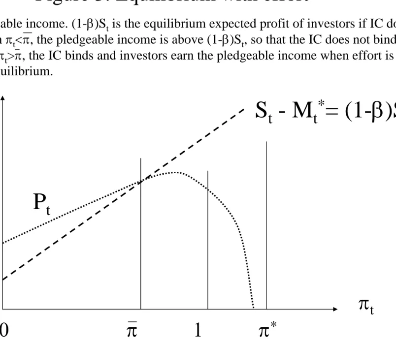
Substracting the rent from the expected output yields the pledgeable income, i.e., the maximum
expected revenue that can be pledged to the investors without compromising the incentives of the
manager:
Since both the expected output and the rent increase with πt, the pledgeable income can be non— monotonic with the expected strength of the speculative sector. Combining the conditions stated
above, we obtain our next proposition.
Proposition 2: When effort is not observable but requested, the pledgeable income in the spec-ulative sector is a concave function P(.)of πt . Moreover if
p+ (1−p)R∆
B < p∆ˆ
∆ , (10)
P(πt) decreases when πtis close enough to 1.
Condition (10) means that the expected negative consequences of shirking are substantially more
important for a fragile industry than for a solid one.12 This condition expresses that pledgeable income
is decreasing at πt= 1.
Proposition 2 implies the following dynamics for the pledgeable income when effort is requested.
As long as high returns are observed, confidence in the speculative sector increases. This boosts
expected output, but it also raises rents. Our assumptions imply that the marginal impact of increased
confidence on pledgeable income decreases withπt(P(πt)is concave). Moreover, under condition (10) the increase in rent ultimately dominates the increase in expected surplus, and pledgeable income
starts decreasing.
4.2
Equilibrium with e
ff
ort
When effort is requested from the agent, there are two possible regimes, depending on whether the
incentive compatibility condition binds or not. In the first regime, the market clearing condition
determines the equilibrium compensation of the managers, as in the previous section, i.e.,
Mt=Mt∗ s.t. G(Mt∗) =F(St−Mt∗)
as in (6). For this to be the equilibrium, it must be that the incentive compatibility condition holds
forMt∗, i.e.,
Mt∗ ≥Rt. (11)
As illustrated in Figure 2, Panel A, in this regime the supply and demand curves on the labour market
intersect above Rt, so that the incentive compatibility condition does not bind.
In the second regime, as illustrated in Figure 2, Panel B, the supply and demand curves on the
labour market intersect below Rt. Thus, the incentive compatibility condition binds, i.e.,
Mt∗ < Rt. (12)
and the expected managerial compensation is
Mt=Rt. (13)
Since this is above M∗
t, managers employed in the speculative sector earn greater expected compen-sation than in the observable effort case. Thus, although they are competitive, they earn a rent. Such
rents make working in the speculative sector very attractive. Indeed the number of managers who
want to work in that sector is above the demand for their services, i.e.,
G(Mt) =G(Rt)> F(St−Mt).
Thus there is rationing in the labour market, as in Shapiro and Stiglitz (1984).
For simplicity consider the case where ν is uniformly distributed over [0,¯ν]and ρis uniform over
[0,¯ρ], i.e., G(ν) = ν ¯ ν, F(ρ) = ρ ¯ ρ.
In that case the market clearing condition (6) definingMt∗ becomes:
M∗ t ¯ ν = St−Mt∗ ¯ ρ . Thus: Mt∗=βS, (14)
where:
β= ν¯ ¯
ν+ ¯ρ ∈[0,1].
The compensation of the manager is equal to a fraction (β) of the value created by the firm. This fraction reflects the relative values of the outside opportunities of managers and investors in the
traditional sector. When managers’ skills in the traditional sector are high, or the opportunities of the
investors in that sector are poor, the market clearing compensation of the managers in the speculative
sector is high.
The condition under which the incentive compatibility condition does not bind, (11), is equivalent
to the condition that the pledgeable income be greater than the expected income of the investors in
thefirst best
St−Mt∗≤Pt. (15)
After some manipulations, we obtain state our next proposition, which is illustrated in Figure 3.
Proposition 3: Consider the case where effort is not observable, but is requested. If F and Gare uniform ,there exists a threshold value π¯ such that, for πt ≤π¯ the incentive compatibility condition
is not binding and the compensation of managers is set by the market clearing condition (6).
• When
B ≤β∆R, (16)
then π¯ º1 and the incentive compatibility constraint never binds. The equilibrium outcome is the same as in the first best.
• When
β∆R < B < β∆ˆpR, (17)
the threshold value ¯π is interior (0<π <¯ 1).For πt>¯π, the compensation of managers is set
Inequality (16) holds when the private benefit from shirking,B, is small. In that case, the moral hazard problem is not large and induces no distortion in equilibrium. Hence, the expected net cashflow
obtained by investors in speculative sector firms is: St−Mt∗.
Inequality (17) holds when B is relatively large and ∆ relatively small. In that case, the agency problem is more severe and, whenπtis high enough, rents become so large that the incentive compati-bility condition binds. Correspondingly, the expected net cashflow obtained by investors in speculative
sector firms is:St−Rt=Pt.
4.3
Equilibrium without e
ff
ort
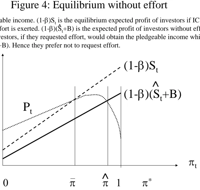
Now turn to the case where effort is not requested from the agent in equilibrium. In that case the
expected output from the project is:
ˆ
St= [πt(1−∆) + (1−πt)p(1−( ˆ∆))]R, and the expected wage earned by managers is
ˆ
Mt= [πt(1−∆) + (1−πt)p(1−( ˆ∆))]mt.
The demand for managers is: F( ˆSt−Mˆt) while he supply of managers is: G( ˆMt+B). The market clearing expected wage without effort isMˆt∗ is such that
F( ˆSt−Mˆt∗) =G( ˆMt∗+B).
Using this market clearing condition, the next proposition states equilibrium wage arising when effort
is not requested.
Proposition 4: Assume F and Gare uniform. If effort is not requested in equilibrium, then the labour market for managers clear, the expected compensation of managers is
ˆ
and their total expected utility is β( ˆSt+B) while that of investors is(1−β)( ˆSt+B).
When effort is not exerted, the total expected value created by each firm is Sˆt+B. Since the agent does not exert effort no rent is needed and the market clears. Thus the share of the total value
created obtained by managers and investors simply reflect their outside options in the traditional
sector. Correspondingly, managers get fraction β of Sˆt+B while investors get the complementary fraction.
4.4
Is there e
ff
ort in equilibrium?
We now investigate if effort is requested in equilibrium. Consider a candidate equilibrium, where effort
is requested. Could a pair manager—investor be better off by deviating to a contract which would
not request effort? If there is no such profitable deviation, then effort is requested in equilibrium.
Symmetrically, consider a candidate equilibrium where effort is not requested. Could a pair manager—
investor be better offby deviating to a contract which would request effort? Again, if there is no such
profitable deviation, there exists an equilibrium without effort. The following proposition, illustrated
in Figure 4, states the conditions on parameter values under which one of the candidate equilibria or
the other prevails.
Proposition 5: Assume F and Gare uniform and (10) and (17) hold. If
R[1−(1−β)(1−∆)]< B[1
∆+ (1−β)]. (18)
there exists a threshold value π >ˆ ¯π such that effort is requested in equilibrium for πt ≤ πˆ, while
equilibrium involves no effort for larger values of πt.
The intuition of the proposition is the following: As long asπt<πˆ, the rents which must be left to the managers are sufficiently small that the pledgeable income is greater than the expected income
investors would get if effort was not requested. So, for these values of πt, investors prefer to request effort, and it is implemented in equilibrium. (18) is the condition under which the threshold valueπˆ is
lower than 1. This condition states that for πt= 1, the pledgeable income is lower than the expected income of the investors when effort is not requested.
5
Discussion and implications
5.1
The lifecycle of the speculative sector
Denote by H(πt) the fraction of the manager’s population employed in the speculative sector. It is a measure of the size of the speculative sector. The above analysis, and in particular Propositions 3, 4
and 5, imply the following corollary.
Corollary 2: As long as there is no crisis, the equilibrium dynamics of the size of the speculative sector, measured by the fraction of the managers employed in that sector, H(πt), is the following:
• For πt<π¯,H(πt) =F((1−β)St),
• for π¯ ≤πt<πˆ,H(πt) =F(Pt),
• and for πˆ ≤πt,H(πt) =F((1−β)( ˆSt+B)).
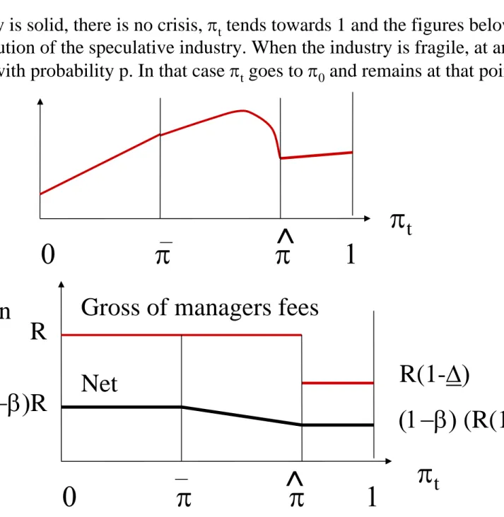
Corollary 2 implies the following pattern for the lifecycle of the financial sector, illustrated in
Figure 5.
• First, as long as there is no crisis,πtgrows (fromπ0toπ¯). This increase in the confidence placed in the speculative sector attracts managers and capital. Correspondingly the total output of the
sector increases. This is the initial boom period following the introduction of the innovation.
• Second, if there is still no crisis, πt continues to grow (from π¯ to πˆ) and managers become so confident that investors must leave them rents to provide them with incentives. As confidence
sector. This deters the allocation of capital to the speculative sector and slows down its growth,
which can even become negative. This is the choking period.
• Third, if the crisis still does not occur, confidence continues to build up, asπtgoes fromπˆtowards 1. But the rents needed to incentivize effort have now grown so high that investors prefer not to
request effort in equilibrium. Consequently, managers screen projects lesss carefully, and failures
take place. As long as the rate of these failures remains as low as ∆, confidence still builds up.
But as soon as the rate of failure exceeds∆, investors realize the sector is fragile, and there is a
crisis.
• At any point in time, if the industry is fragile, this can be revealed, either by a large crisis implying the failure of the entire speculative sector, or by a large average failure rate ∆¯ in the speculative industry. In both cases, confidence is destroyed andπtdrops to 0, where it remains. At that point, the size of the speculative sector and the wages in that sector undergo a sharp
drop.
5.2
Risk and the speculative sector
There are two types of risk in our setting. First, there is the risk of a crisis affecting the whole
speculative sector. Second, there is the micro—risk affecting an individual project when its manager
shirked. We discuss them in turn.
First, consider the aggegate risk. The occurrence of the corresponding crisis is exogenous in our
model. What is endogenous is the perception of that risk by agents, and their rational updating about
the probability of crises. As the sequence of positive returns grows longer, risk is perceived to decline
by all market participants. But in our simple framework, it takes only one shock for the confidence
in the speculative sector to be entirely lost. It would be straightforward to extend our model to allow
for a more gradual process. Suppose that the probability of a crisis is p when the industry is fragile and when it is strong, with p > >0. After the observation of afirst shock,πt would go down but
would not immediately reach 0. Then, after each crisis episode, market participants would become
more and more pessimistic andπt would progressively go to 0.
Second, consider the micro—shock, corresponding to the failure of one project. It is endogenous in
our model, since when the agent exerts effort this risk is lower than when the agent shirks. In the
case of the financial industry, effort can be interpreted as the hard work necessary to evaluate the
creditworthiness of investment projects and screen out the bad ones. If bankers and fund managers
don’t exert this effort, it raises the risk that they allocate money to bad loans or unprofitable assets,
and thus will fail. Thus, towards the end of the cycle, asπtbecomes larger thanπˆ, the risk that many speculative projects fail increases in equilibrium. As it affects manyfirms simultaneously, this can be
interpreted as systemic risk.
5.3
Empirical implications for the
fi
nancial industry
In this subsection, we draw the empirical implications of our theoretical analysis for the financial
industry. Our model is not relevant for all parts of thefinancial industry and all periods. It applies to
segments and periods corresponding to our definition of a speculative industry: there is a significant
innovation involving both risks and promises, it is quite uncertain whether the innovation is strong or
fragile, and informational asymmetries between investors andfinance sector managers are severe. Thus,
our model does not apply to standard banking activities, such as loans to corporations, conducted
in traditional ways, during periods with little financial innovation, e.g., the 1950s or the 1960s. In
contrast, it is relevant to analyze theflow offinancial innovations which took place at the beginning of
this century or for previous waves offinancial innovations, such as, e.g., that of the 1920s. To delineate
the implications of our theoretical analyses for such situations, we rely mainly on the equilibrium
dynamics illustrated in Figure 5.
Rents: Our model implies that duringfinancial innovation waves, after the industry has acquired
would receive in a frictionless market. These rents arise in equilibrium, in spite of competition between
managers, because of incentive constraints, in line with Shapiro and Stiglitz (1984).
This theoretical result is consistent with the empirical findings of Philippon and Reshef (2008).
They observe that during the 1920s and after the 1980s, there was a burst of financial innovation, an
increase in the complexity offinancial jobs, and also an increase in the pay of managers in thefinance
sector increased. Philippon and Reshef (2008) estimate that, in the recent period, rents accounted for
30% to 50% of the wage differential between the financial sector and the rest of the private sector.
They also find that this induced an increase in involuntary unemployment in the financial industry.
Our theoretical analyses delivers results which are exactly in line with these facts.
Another implication of our model is that, as confidence in the financial innovation builds up,
compensation contracts in the innovative financial sector should become more and more favorable
to fund managers (at the expense of investors). This is a new implication, which has not yet been
tested systematically. But it is consistent with anecdotal evidence from private equity funds that,
at the beginning of this century, on top of the 2 percent annual management fee and the carried
interest incentive fee, extra fees were progressively added, sometimes labeled portfolio fees. These fees
progressively reduced the net performance earned by investors (see Phalippou, 2008).
Net returns and size: The equilibrium dynamics characterized above imply that, as long as
there is no crisis, realized returns net of management fees, start at a high level and then go down with past performance. While realized net returns are non—increasing, expected net returns initially increase. This is because the increase in the probability of success outweighs the increase in fees.
The corresponding increase in expected net returns attracts capital. Hence the size of the sector
(measured, e.g., by assets under management or total open positions) initially increases with past
performance. Thus, during that period, an increase in size coexists with a decrease in realized net
returns, which can be interpreted in terms of decreasing marginal returns to size.13 But, at some
1 3This is reminiscent of the results of Berk and Green (2005), but obtains for different reasons. In the present model,
point the increase in agency rents can outweigh the increase in confidence and expected net returns
themselves start decreasing. When that point is reached, investment in the speculative sector declines.
Thus, overall, the relationship between the amount of money invested in the speculative sector and
its past performance will be inverse U shaped. This implication from our theoretical analysis is in
line with the empirical results of Ramadorai (2008). He studies the closed—fund premium in the hedge
fund industry. This premium offers a proxy for the demand for hedge—fund management services.
When it is large, it suggests that many investors are eager to delegate the management of their money
to that segment of the speculative financial industry. Consistent with our models, Ramadorai (2008)
finds that this premium is initially increasing and then decreasing with past performance.
Managers’ skills: In our model, as the size of the speculative sector increases, it attracts better
and better managers. This implication of our analysis is in line with the empiricalfindings of Philippon
and Reshef (2008) that the average skill level of managers in thefinancial services industry rose at the
beginning of this century.
Time— and money—weighted average returns: During the ascending phase of the cycle the
size of the speculative sector goes up. Hence time—weighted average returns give more weight to early
returns than do money—weighted averages. Now, as shown above, even if there is no crisis, realized
net returns tend to decrease. Hence the time—weighted average net return is greater than the money—
weighted one. And the former overestimates further returns more than the latter. Thus our model
warns that investors should view past time—weighted average net returns with caution, and should not
extrapolate them, since this would neglect the growth in agency rents.
Estimating risk: Our learning model is a good description of industries, such as the financial
one recently, where until some rare event occurs there is no strong change in beliefs, and then when
of learning, moral hazard and equilibrium effects. Also, managers in our model are identical, while they are heterogeneous in Berk and Green (2005).
the rare event happens, there is a strong decline in optimism. In such an environment, frequentist
estimations of risk would be very misleading. Consider the case where, up to time t, there has been no crisis. The estimated default rate computed using past data is 0. This is lower than the rational
Bayesian estimate of the risk of default which is
1−(πt+ (1−πt)p)>0.
This is in line with the analysis of the recent crisis offered by Brunnermeier (2009) and Rajan et al
(2008). Brunnermeier (2009) notes that: “the statistical models of many professional investors and
credit-rating agencies provided overly optimistic forecasts about structured finance products. One
reason is that these models were based on historically low mortgage default and delinquency rates.”
6
Conclusion and policy implications
Our model analyzes the lifecycle of speculative industries, exploiting innovations and characterized by
uncertainty about the fundamental value of these innovations, as well as information asymmetry about
the actions of the managers implementing them. These assumptionsfit particularly well the evolution
of the financial industry at the beginning of this century. And our theoretical analysis delivers a
rich set of empirical implications, in line with the evolution of that industry and its eventual crisis.
In particular our model shows how, in equilibrium, during the initial period of success, the industry
grows, attracting human and financial capital, while the rents of the managers increase. Our model
also shows how this increase in rents undermines the net returns obtained by investors and eventually
makes incentives so expensive that excessive risk—taking prevails in the last part of the cycle.
In our analysis optimal contracts preclude large managerial compensation after failure. Thus,
under our assumptions, the large compensations recently warranted tofinancial sector executives were
suboptimal, and exacerbated agency and risk taking problems. Our analysis also implies that disclosure
and transparency, to the extent that they reduce the private benefit from shirking, alleviate the moral
increasing investors’ net returns and ii) enlarging the set of parameters for which suboptimal risk—
taking is deterred in equilibrium. Along with this advice to policy makers, our analysis also offers
a warning: Even with the maximum possible level of disclosure and optimal contracts, rents and
References:
Barbarino, A., and B. Jovanovic, 2007, “Shakeouts and market crashes,”International Economic Review, 385—420.
Berk, J., and R. Green, 2005, “Mutual fundflows and performance in rational markets,” Journal of Political Economy.
Bergemann, D., and U. Hege, 1998, “Dynamic Venture Capital Financing, Learning and Moral
Hazard,” Journal of Banking and Finance, 703-735.
Brunnermeier, M., 2009, “Deciphering the Liquidity and Credit Crunch 2007—2008,” Journal of Economic Perspectives, 77—100
DeMarzo,P., and Y.Sannikov, 2008, “Learning in Dynamic Incentive Contracts” Working paper,
Stanford University.
Holmstrom, B., and J. Tirole, 1997, “Financial intermediation, loanable funds and the real sector,”
Quarterly Journal of Economics, 663—692.
Lorenzoni, G., 2008, “Inefficient credit booms,” Review of Economic Studies, 809—833.
Pastor, L., and P. Veronesi, 2006, “Was there a Nasdaq bubble in the late 1990’s ?,” Journal of Financial Economics., 81, 161—100.
Phalippou, L., 2008, “Beware of venturing into private equity,”Journal of Economic Perspective, Volume 22, Number 4.
Philippon, T., 2008, “The evolution of the US financial industry from 1860 to 2007: Theory and
evidence,” Working paper, New York University.
Philippon, T., and A. Reshef, 2008, “Skill biased financial development: education, wages and
occupations in the U.S. financial sector”, Working paper, New York University.
Rajan, U., A. Seru, and V. Vig, 2008, “The Failure of Models that Predict Failure: Distance,
Incentives and Defaults,” Working paper, University of Michigan at Ann Arbor.
Working paper, Saïd Business School, Oxford University.
Rob, R., 1991, “Learning and capacity expansion under demand uncertainty.”Review of Economic Studies, 655—677.
Shapiro, C. and J. Stiglitz, 1984, “Equilibrium Unemployment as a Worker Discipline Device,”
The American Economic Review, 74, 433 — 444.
Zeira, J., 1987, “Investment as a process of search.”Journal of Political Economy, 204—210. Zeira, J., 1999, “Informational overshooting, booms and crashes.”Journal of Monetary Economics, 237—257.
Appendix: Proofs
Proof of Proposition 2:
Substituting the values of St from (3) and Rt from (7), the pledgeable income at time t can be written as a function of πt: Pt=P(πt) = [p+ (1−p)πt][R+ B [p∆ˆ −∆](πt−π∗) ], where π∗ = p∆ˆ p∆ˆ −∆.
Note that, underA1:
π∗>1.
Thefirst derivative of the pledgeable income is:
P0(πt) = (1−p)R−B
p+ (1−p)π∗
[p∆ˆ −∆](πt−π∗)2
,
while the second derivative is:
P00(πt) = 2B
p+ (1−p)π∗
[p∆ˆ −∆](πt−π∗)3
.
Thus, P00(πt) < 0 for the relevant values of πt, i.e., πt ≤ 1 < π∗. Thus the pledgeable income as a function of πt is a hyperbola, concave forπt∈[0,1].
Now, P0(1)<0⇔(1−p)R < B p+ (1−p)π ∗ [p∆ˆ −∆](1−π∗)2. That is: (1−p)R < pB∆ˆ −∆) ∆2 .
Or: p+ (1−p)R∆ B < p ˆ ∆−∆) ∆ .
Hence the proposition.
QED
Proof of Proposition 3:
Substituting the market clearing managerial compensation (14) into (15), we obtain
(1−β)St≤Pt, that is: (1−β)[p+ (1−p)πt]R≤[p+ (1−p)πt]R− [p+ (1−p)πt]B p∆ˆ −πt[ ˆ∆p−∆] .
Simplifying both sides byp+ (1−p)πtand rearranging terms, we obtain a much simpler condition:
βR≥ B
p∆ˆ −πt[ ˆ∆p−∆]
. (19)
which is satisfied for πt small enough. Note also that, if B ≤β∆R, condition (19) holds at πt= 1, and therefore for all πt. In contrast, if β∆R < B < β∆ˆpR, condition (19) holds atπt= 0, but not at
πt= 1. QED
Proof of Proposition 4:
In the uniform distribution case, the market clearing condition without effort amounts to
Mt∗+B ¯ ν = ˆ St−Mt∗ ¯ ρ . That is Mˆt∗+B = ρν¯¯( ˆSt−Mˆt∗).Or ˆ Mt∗(1 + ¯ν ¯ ρ) +B = ¯ ν ¯ ρSˆt.
That is ˆ Mt∗= ν¯ ¯ ρ+ ¯ν ˆ St− ¯ ρ ¯ ρ+ ¯νB =β ˆ St−(1−β)B.
Hence the expected total gain of the manager isMˆt∗+B=βSˆt−(1−β)B+B=β( ˆSt+B). Similarly, the expected profit of the investors isSˆt−Mt∗ = (1−β)( ˆSt+B).
QED
Proof of Proposition 5:
The preliminary step of the proof is to compare the following three functions of πt: (1−β)St,
(1−β)( ˆSt+B) and Pt. Note the following:
• (1−β)St and (1−β)( ˆSt+B) are linear and increasing inπt .
• (17) implies that, atπt= 0,P(πt= 0)>(1−β)S(πt= 0).
• A1 and A2 imply that (1−β)St>(1−β)( ˆSt+B).
• (10) implies that Pt is concave inπt, increasing at 0 and decreasing at 1.
• By (10) and (17), there exists a threshold value π¯ ∈[0,1] such that: P(πt) <(1−β)St if and only if πt>π¯.
• P(πt)<(1−β)( ˆSt+B) holds forπt= 1if and only if R− B∆ <(1−β)[(1−∆)R+B], which simplifies to condition (18).
This implies that under condition (18) there exists a threshold valueπˆ∈[0,1]such that: P(πt)<
(1−β)(St+B) if and only ifπt>πˆ. Also, since(1−β)St>(1−β)( ˆSt+B), we have thatπ >ˆ π¯. The functions(1−β)St,(1−β)( ˆSt+B)andPtare plotted in Figure 4. The remainder of the proof consists in three steps, each one considering a candidate equilibrium and spanning the different possible values
of πt.
First, we consider the case where πt < π¯ and establish, that in that case, effort is requested in equilibrium. Since πt < π¯, the incentive compatibility condition does not bind. In the candidate
equilibrium, the total expected value created by the firm is St, and investors receive (1−β)St while managers receive βSt. If a pair manager-investor were to deviate to a contract without effort, this would generate total expected value equal to Sˆt+B. Under A1 and A2, Sˆt+B < St. Hence it is impossible to design a contract requesting no effort to which both the manager and the investor would
prefer to deviate. Consequently, for πt<π¯, there is an equilibrium with effort.
Second, turn to the case whereπ > πˆ t >π¯. As in the previous case consider a candidate equilib-rium with effort and take a similar approach: In that candidate equilibequilib-rium, the investor receives in
expectationPtand the managerRt. The sum of the two isSt. Could a manager and an investor both prefer to deviate to a contract with effort? In that deviation, the total value created by thefirm would
be Sˆt+B. Under A1 and A2, this is lower than the total value created in the candidate equilibrium
St. Hence, the investor could not both agree to such the deviation. Consequently, for π > πˆ t > π¯, there is an equilibrium with effort.
Third, focus on the case whereπt>π >ˆ π¯. Consider a candidate equilibrium without effort. In that candidate equilibrium, the investor receives in expectation (1−β) ˆSt and the manager βSˆt. Could a manager and an investor both prefer to deviate to a contract with effort? In that deviation, the investor
could at most get P(πt). Now, by construction of πˆ, we have P(πt) < (1−β) ˆSt,∀πt > πˆ. Hence, the investor could not agree to such a deviation. Consequently, for πt > ˆπ, there is an equilibrium without effort.