Abstract Test Case Prioritization Using
Repeated Small-Strength Level-Combination
Coverage
Rubing Huang, Weifeng Sun, Tsong Yueh Chen,
Dave Towey, Jinfu Chen, Weiwen Zong, Yunan Zhou
Faculty of Science and Engineering, University of Nottingham Ningbo
China, 199 Taikang East Road, Ningbo, 315100, Zhejiang, China.
First published 2020
This work is made available under the terms of the Creative Commons
Attribution 4.0 International License:
http://creativecommons.org/licenses/by/4.0
The work is licenced to the University of Nottingham Ningbo China
under the Global University Publication Licence:
https://www.nottingham.edu.cn/en/library/documents/research-support/global-university-publications-licence.pdf
Abstract Test Case Prioritization using Repeated
Small-strength Level-combination Coverage
Rubing Huang,
Member, IEEE,
Weifeng Sun, Tsong Yueh Chen,
Senior Member, IEEE,
Dave
Towey,
Member, IEEE,
Jinfu Chen,
Member, IEEE,
Weiwen Zong, Yunan Zhou
Abstract—Abstract Test Cases (ATCs) have been widely used in practice, including in combinatorial testing and in software product line testing. When constructing a set of ATCs, due to limited testing resources in practice (for example in regression testing), Test Case Prioritization (TCP) has been proposed to improve the testing quality, aiming at ordering test cases to increase the speed with which faults are detected. One intuitive and extensively studied TCP technique for ATCs isλ-wise Level-combination Coverage based Prioritization(λLCP), a static, black-box prioritization technique that only uses the ATC information to guide the prioritization process. A challenge facingλLCP, however, is the necessity for the selection of the fixed prioritization strengthλbefore testing — testers need to choose an appropriateλvalue before testing begins. Choosing higherλvalues may improve the testing effectiveness ofλLCP (for example, by finding faults faster), but may reduce the testing efficiency (by incurring additional prioritization costs). Conversely, choosing lowerλvalues may improve the efficiency, but may also reduce the effectiveness. In this paper, we propose a new family of λLCP techniques,Repeated Small-strength Level-combination Coverage-based Prioritization(RSLCP), that repeatedly achieves the full combination coverage at lower strengths. RSLCP maintainsλLCP’s advantages of being static and black box, but avoids the challenge of prioritization strength selection. We performed an empirical study involving five different versions of each of five C programs. Compared withλLCP, andIncremental-strength LCP(ILCP), our results show that RSLCP could provide a good trade-off between testing effectiveness and efficiency. Our results also show that RSLCP is more effective and efficient than two popular techniques ofSimilarity-based Prioritization(SP). In addition, the results of empirical studies also show that RSLCP can remain robust over multiple system releases.
Index Terms—Software testing, regression testing, abstract test case, test case prioritization, level-combination coverage.
F
1
I
NTRODUCTIONI
N practice, software systems are usually influenced by different parameters or factors (such as configuration op-tions and user inputs), with each parameter possibly having a finite set of differentlevelsorvalues. An abstract test case (ATC) represents a combination of levels of different pa-rameters, and has been used in different testing situations, including combinatorial testing [1], software product lines testing [2], and highly-configurable systems testing [3].When an ATC set has been constructed, it is desirable to execute all the test cases — in which case execution order does not matter. However, due to often limited testing resources, it is often possible to only run some of the ATCs in the set. In such situations, the ATC execution order may become critical, because a well-prioritized test case
• R. Huang is with the School of Computer Science and Communication Engineering, and also with Jiangsu Key Laboratory of Security Technology for Industrial Cyberspace, Jiangsu University, Zhenjiang, Jiangsu 212013, China.
E-mail: [email protected].
• W. Sun, J. Chen, W. Zong, and Y. Zhou are with the School of Computer Science and Communication Engineering, Jiangsu University, Zhenjiang, Jiangsu 212013, China.
E-mail: [email protected], {jinfuchen, vevanzong, zhouyn}@ujs.edu.cn.
• T. Y. Chen is with the Department of Computer Science and Software Engineering, Swinburne University of Technology, Hawthorn, VIC 3122, Australia.
E-mail: [email protected].
• D. Towey is with the School of Computer Science, University of Notting-ham Ningbo China, Ningbo, Zhejiang 315100, China.
E-mail: [email protected].
execution sequence may identify failures more quickly, and thus may enable earlier fault characterization, diagnosis and correction [1]. Generally speaking, the process of schedul-ing the order of test cases is called Test Case Prioritization
(TCP) [4], and the prioritization of ATCs is calledAbstract Test Case Prioritization(ATCP) [5].
Many strategies have been proposed to guide ATCP according to different criteria, for examplerandom test case prioritization[6, 7], andSimilarity-based Prioritization(SP) [8– 10]. The most widely-used ATCP isλ-wise Level-combination Coverage-based Prioritization (λLCP) [11], which adopts a fixed strengthλ(called theprioritization strength) to choose each ATC in a greedy manner: When selecting each next ATC from the candidates, λLCP calculates the number of parameter-level combinations at a fixed prioritization strengthλcovered by each candidate that has not yet been covered by executed test cases, and then chooses the one with the maximum number of uncoveredλ-wise parameter-level combinations.λLCP has many advantages, including that it is simple and intuitive [11]. Furthermore, because it only uses the level-combination coverage information derived from the test cases, rather than information from the source code or program execution,λLCP is a static, black-box technique [12]. Although previous studies have shown thatλLCP is an effective prioritization technique, in terms of fault detection [6, 11, 13, 14], it does have a constraint that the fixed strengthλmust be set before prioritization begins. Differentλvalues may lead to different performances, with investigations [13, 14] finding that larger λ values may improve the testing effectiveness ofλLCP (for example, by
finding faults faster), but may reduce the testing efficiency (by incurring additional prioritization costs); conversely, lower λ values may improve the efficiency, but may also reduce the effectiveness.
Although it is intuitive that a small prioritization strength forλLCP may be efficient (in terms of overheads), it has also been shown that over 50% of faults can be triggered by one parameter (1-wise combination coverage), and more than 70% can triggered by two (2-wise combina-tion coverage) [15, 16]. This indicates that choosing a small prioritization strength may be effective forλLCP, especially when the number of ATCs is small. However, when the ATC candidate set is large,λLCP with small prioritization strengths may become ineffective [17]. This is because, when the small-strength (1-wise or 2-wise) level-combination cov-erage is fully achieved by the selected or executed ATCs, the remaining candidates are effectively randomly ordered.
In this paper we propose a new family of λLCP tech-niques, Repeated Small-strength Level-combination Coverage-based Prioritization (RSLCP). RSLCP attempts to overcome the limitations of current versions of LCP, attempting to better balance the trade-off between testing effectiveness and efficiency. In particular, RSLCP begins with a small prioritization strengthλ(λ= 1,2)to implement theλLCP algorithm — which means that RSLCP is also initiallyλLCP. Once theλ-wise level-combination coverage of selected or executed ATCs is fully achieved — i.e., the number ofλ-wise level combinations covered by the selected ATCs is equal to that covered by all candidates — then RSLCP restarts with the same prioritization strength λ, repeating full λ -wise level-combination coverage in the next round. This process is repeated until all candidates have been chosen. RSLCP has the following three advantages: (1) it is very simple, adopting a similar mechanism toλLCP; (2) similar toλLCP, it is a static, black-box prioritization method, using only the level-combination coverage to guide the ATCP (this means that it is not necessary to obtain source code information, nor to execute the program); and (3) unlike λLCP, it is not necessary to set the prioritization strength before prioritizing ATCs.
To evaluate the proposed technique, we conducted em-pirical studies on five C programs, each of which had five different versions. In summary, the main contributions of this paper are:
• We propose a new strategy to guide the ATC prioriti-zation,Repeated Fixed-small-strength Level-combination Coverage-based Prioritization(RSLCP), and describe a framework to support it.
• Based on the proposed framework, we provide two categories (using two different strategies) involving six algorithms to implement RSLCP.
• We report on empirical studies investigating each RSLCP technique, comparing with λLCP and SP, from the perspectives of: testing effectiveness (the speed of interaction coverage and fault detection); testing efficiency (the prioritization cost); and robust-ness (how well the overall fault detection potential is maintained across different versions of the software under test).
The rest of this paper is organized as follows: Section 2
describes the background information. Section 3 introduces the RSLCP method, including the framework, algorithm, complexity analysis, and mechanism. Section 4 presents the research questions and experimental setup. Section 5 reports on the empirical studies conducted to answer the research questions. Section 6 reviews related work, and, finally, Section 7 concludes the paper, and discusses future work.
2
B
ACKGROUNDIn this section, we describe some background information about abstract test cases and test case prioritization.
2.1 Abstract Test Case
Given some software under test (SUT) that haskparameters that constitute a parameter setP = {p1, p2,· · ·, pk}, with a corresponding level set L = {L1, L2,· · · , Lk}, where each parameterpi has some valid levels from the finite set Li (i = 1,2,· · · , k). In practice, parameters may represent anything that influences the performance of the SUT, such as components, configuration options, user inputs, and so on. LetQbe the set of constraints on level combinations. Definition 2.1. Input Parameter Model: An input
pa-rameter model (or input model) for the SUT, denoted as Model(P, L,Q), is a model of the SUT that includes the set of some parametersP that may influence the SUT, the set of level setsLfor each parameter, and constraints setQon level combinations.
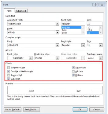
For example, Figure 1 shows a screenshot of the font settings for Microsoft Word 20131. As shown in the red
box, we only consider the Effects aspects of the font set-tings, for which there are seven choices. Table 1 gives an
1. https://products.office.com/en-us/microsoft-word-2013.
TABLE 1
An Input Parameter Model for Microsoft Word 2013 Font Effects.
Parameter p1:Strikethrough p2:Double Strikethrough p3:Superscript p4:Subscript p5:Small caps p6:All caps p7:Hidden
Level Yes(0) Yes(2) Yes(4) Yes(6) Yes(8) Yes(10) Yes(12)
No(1) No(3) No(5) No(7) No(9) No(11) No(13) (Strikethrough= “Yes”)↔(Double Strikethrough= “No”), i.e.,(p1= “0”)↔(p2= “3”).
(Superscript= “Yes”)↔(Subscript= “No”), i.e.,(p3= “4”)↔(p4= “7”).
(Small caps= “Yes”)↔(All caps= “No”), i.e.,(p5= “8”)↔(p6= “11”). input parameter model for the font effects of Microsoft Word 2013. The effects have seven parameters, each of which can have two levels. It is not possible to have both parameters from any of the sets (Strikethrough, Double Strikethrough), (Superscript, Subscript), or (Small caps,
All caps) to be “Yes” at the same time. Therefore, there are three level combination constraints. To simplify the rep-resentation of this problem, each parameter can be denoted bypi(i= 1,2,· · · ,7), and each level can be labelled by an integer (starting at0), as shown in Table 1.
This example yields the following input parameter model: Model(P = {p1, p2,· · · , p7}, L = {{“0”,“1”},
{“2”,“3”},{“4”,“5”},{“6”,“7”},{“8”,“9”},{“10”,“11”},
{“12”,“13”}},Q = {p1 = “0” ↔ p2 = “3”, p3 =
“4” ↔ p4 = “7”, p5 = “8” ↔ p6 = “11”}), where
the symbol ↔ represents implication. Because the specific values of each parameter have no impact on the SUT model, without loss of generality, we can use the following abbreviated version: Model(|L1||L2| · · · |Lk|,Q). Therefore, the above model can be represented as:
Model(27,Q={“0”↔“3”,“4”↔“7”,“8”↔“11”}). Definition 2.2.Abstract Test Case:A k-tuple(l1, l2,· · · , lk)
is an abstract test case of the SUT whereli∈Li,1≤i≤k. If all the level constraints in Q are satisfied, then the ATC is said to be valid, otherwise it is invalid. An example of a valid ATC for the previous model is
(“0”,“3”,“4”,“7”,“8”,“11”,“12”); and an example of an invalid one is (“0”,“2”,“5”,“6”,“9”,“10”,“13”) — be-cause it violates the constraint(“0”↔“3”).
Definition 2.3. η-wise Level Combination:An η-wise level combination is ak-tuple(bl1,bl2,· · ·,blk)involving η
param-eters with fixed levels (called fixed paramparam-eters) and(k−η) parameters with arbitrary allowable levels (called free param-eters that are denoted by “−”), where0≤η≤kand:
b
li=
{
li∈Li, ifpiis a fixed parameter;
−, ifpiis a free parameter (1)
An η-wise level combination is also called an η-wise schema [1]. Without loss of generality, to more clearly de-scribe the problem, free parameters can be ignored. In other words, an η-wise level combination can be consid-ered an η-tuple. Intuitively speaking, any ATC can cov-er some η-wise level combinations: for example, an ATC
(“1”,“2”,“4”,“7”,“8”,“11”,“13”)covers seven 1-wise lev-el combinations(“1”),(“2”),(“4”),(“7”),(“8”),(“11”), and
(“13”). Similar to ATCs, anη-wise level combination may
also be either valid or invalid: for example, a 2-wise level combination(“1”,“2”)is valid; but another one,(“0”,“2”), is invalid. Obviously, a valid ATC covers all valid η-wise level combinations, regardless ofηvalues.
For ease of description, we define a functionψ(η, tc)for an ATCtcthat returns the set of allη-wise level combina-tions covered bytc, i.e.:
ψ(η, tc) ={(vj1, vj2,· · ·, vjη)|1≤j1< j2<· · ·< jη≤k} (2) Similarly, a functionψ(η, T)for a set T of test cases can be defined to return the set of allη-wise level combinations covered by all model inputs inT, i.e.:
ψ(η, T) = ∪
tc∈T
ψ(η, tc) (3)
Obviously, the size ofψ(η, tc)(|ψ(η, tc)|) is equal toC(k, η) (the number ofη-combinations fromkelements).
We next present the definition of η-wise level-combination coverage for an ATC, or for a subset of the given test set.
Definition 2.4.η-wise Level-combination Coverage:Given a valid test suite T, a valid ATCtc, and a subsetT′ of T (tc∈T andT′ ⊆T), theη-wise level-combination coverage of tcagainst T can be defined as the ratio of the number of η-wise level combinations covered bytcto those covered byT:
|ψ(η,tc)|
|ψ(η,T)|. Theη-wise level-combination coverage of test setT′ againstT can be written as: ||ψψ((η,Tη,T′))||.
2.2 Test Case Prioritization
Test Case Prioritization (TCP) seeks to schedule test cases such that those with higher priority, according to some criteria, are executed earlier than those with lower priority. When testing resources are limited or insufficient for the execution of all test cases in a test suite, a well-designed test case execution order can be crucial. The problem of Test Case Prioritization is defined as follows [4]:
Definition 2.5.Test Case Prioritization:Given a tuple(T,Ω, g),
whereT is a test suite,Ωis the set of all possible permutations of
T, andgis a fitness function fromΩto real numbers, the goal of
test case prioritization is to find a prioritized test suite (also called
a test sequence)S ∈Ωsuch that:
(∀S′) (S′∈Ω) (S′̸=S) [g(S)≥g(S′)] (4)
According to Rothermel et al. [4], prioritization can be done according to many possible criteria, including, for example, code coverage [18]. To date, many TCP strategies have been proposed, based on various concepts, including: fault severity [19]; source code coverage [4, 20, 21]; search-based techniques [18]; integer linear programming [22]; risk exposure [23]; historical records from recent regression tests [24]; and information retrieval [25, 26]. Most strategies can be classified as either meta-heuristic search methods or greedy methods [27]. When TCP is applied to abstract test cases, it is calledAbstract Test Case Prioritization(ATCP) [5].
3
R
EPEATEDF
IXED-
SMALL-
STRENGTHL
EVEL-COMBINATION
C
OVERAGE-
BASEDP
RIORITIZATIONIn this section, we present a new family ofλLCP techniques that work by repeatedly using repeated, small-strength level-combination coverage. We call these techniques Re-peated Small-strength Level-combination Coverage-based Priori-tization(RSLCP). We introduce two RSLCP versions in this section, and present an analysis of the space and time complexity for each version.
3.1 Framework
Unlike λLCP, because the RSLCP prioritization strength is limited to 1 or 2, it is not necessary that a value be assigned toλbefore prioritizing ATCs.
As shown in Figure 2, RSLCP prioritizes an unordered set of ATCs (denoted T) into a prioritized set S that has been divided into α (α ≥ 1) disjoint and ordered parts
⟨S1, S2,· · ·, Sα⟩, where each Si (i = 1,2,· · ·, α) has also been prioritized using a prioritization strengthλi. Formally, the following five conditions must be satisfied:
1)EachSiis a non-empty test sequence,1≤i≤α;
2)T =S1∪S2∪· · ·∪Sα;
3)S=⟨S1, S2,· · ·, Sα⟩;
4)Si∩Sj=∅,1≤i̸=j≤α;
5)λiis used for the construction ofSi
(5)
Condition 1 means each subsetSiis both non-empty and ordered. Condition 2 means that all test cases are divided amongst theαsubsets. Condition 3 means thatSis ordered by sequencing S1, S2,· · ·, Sα successively (which means thatSj+1followsSj (1≤j < α)). According to Condition 4, no test case belongs to more than one test sequence, and, finally, Condition 5 means that Si is constructed using the prioritization strengthλi.
Although the value ofαis fully determined by the given T, it does not impact on the framework or on the following algorithms. We created two versions of the framework, an
independentand apartially-independentversion.
3.1.1 RSLCP Independent Version
The RSLCP Independent Version (RSLCP-IV) guarantees that construction ofSi+1 is independent of construction of Si(1≤i < α). Formally, the following two conditions must be satisfied: 1)λl∈ {1,2},1≤l≤α; 2)ψ(λl, Sl) =ψ(λl, T\∪li−=11Si) (6)
Condition 1 means that each subset Si adopts a small strength (1 or 2) to guide the λLCP process. Condition 2 means that each subset Si covers allλi-wise level combi-nations that could be covered by the candidates remaining before constructingSi.
Although the construction of test sequences Si and Si+1 (1 ≤ i < α) are independent, actually, construction
ofSimay impact on the construction ofSi+1(becauseSi+1
is constructed using only those test cases remaining after Si’s construction). The algorithms used to prioritize each test sequenceSiwill be presented in Section 3.2.
6 6 ȜZLVH ȜZLVH 6Į 6Į ȜĮZLVH 6 ȜĮZLVH Fig. 2. Illustration of RSLCP. 3.1.2 RSLCP Partially-independent Version
The RSLCP Partially-independent Version (RSLCP-PV) is similar to the independent version, but involves some Si+1 constructions that are based on the Si construction. The following three conditions must be satisfied (assuming S0=∅): 1)λ2x−1= 1, λ2x= 2,1≤x≤ ⌈α2⌉; 2)ψ(λ2x−1, S2x−1) =ψ(λ2x−1, T\∪2i=1x−2Si); 3)ψ(λ2x, S2x−1∪S2x) =ψ(λ2x, T\∪2i=1x−2Si) (7) wherexis an integer.
Condition 1 differs from that of RSLCP-IV by assigning a prioritization strength of 1 to each Si when i is an odd number, and a strength of 2 wheniis even. Conditions 2 and 3 mean that, wheniis odd, the corresponding test sequence Si is constructed independently to achieve the highest 1-wise level-combination coverage; but wheniis even, theSi is constructed so as to guarantee that Si and Si−1 cover
the same 2-wise level combinations as those covered by the remaining candidates. In effect, RSLCP-PV first uses a prioritization strength of 1 to construct the subset S2x−1,
and then considersS2x−1 as the already selected ATCs for
construction of the test sequence S2x. This process is then repeatedly applied to the remaining candidates.
3.2 Algorithm
Algorithm 1 describes the basic RSLCP procedure, which includes iteratively constructing each Si (i = 1,2,· · ·, α) (Line 4). Once anSiis completely constructed, it is added to the end ofS (S ←S ≻Si) (Line 5), and removed from the candidate setT′ (Line 6). The test sequenceSi+1 can then
be constructed, with such constructions continuing until all candidates have been chosen. Clearly, although construction of the test sequence Si is independent of construction of Sj (1 ≤ i ̸= j ≤ α), as can be seen, because Sj is constructed using elements from candidates remaining after
Algorithm 1:RSLCP Procedure
Input: T ={tc1, tc2,· · ·, tcn} ◃Unordered ATCs
Output: S ◃Prioritized ATCs
1: i←1 2: T′←T
3: while|S| ̸=ndo
4: ConstructSiby selecting elements from the remaining candidates T′as subsequent ATCs inS, according to a specified criterion and λi∈ {1,2}, i.e., Algorithm2(T′, λi)or Algorithm3(T′, λi).
5: S←(S≻Si) ◃AddSiinto the end ofS
6: T′←(T′\Si)
7: i←(i+ 1) 8: end while
Si’s construction, the construction of Si can impact that of Sj.
We propose an algorithm to complete the construction process for each Si. The algorithm draws from the well-known greedy approach, Additional Greedy Approach [18], which iteratively selects the element of maximum weight (for the problem) from those parts not yet selected or executed. The problem for construction of Si is to cover the maximum number of λi-wise level combinations not yet covered by test cases that have already been selected or executed. Algorithm 2 describes the Additional Greedy algorithm to construct Si for RSLCP-IV, and Algorithm 3 describes it for RSLCP-PV.
3.2.1 RSLCP-IV Algorithm
As shown in Algorithm 2, the RSLCP-IV algorithm chooses one of the candidates as the next ATC in Si such that it covers the maximum number ofλi-wise level combinations that have not yet been covered by the already selected or executed ATCs in Si (Line 5). If more than one candidate has the highest λi-wise level-combination coverage, then a random tie-breaking mechanism [28] is used, so that one best candidate is selected. This process is repeated until either of the following two conditions is satisfied (Line 3): (1) all candidates have been selected (i.e., T′ = ∅); or (2) Siachieves fullλi-wise level-combination coverage against T′ (i.e., ψ(λi, Si) = TempSet, where TempSet is the set of λi-wise level combinations covered by the remaining ATCs after completely constructingSi−1).
For each prioritization strength λi (1 ≤ i ≤ α) used for constructing Si, we use the following five assignment categories:
• Pure 1-wise RSLCP-IV: Each prioritization strength λiis assigned a value of 1:λ1=λ2=· · ·=λα= 1.
• Pure 2-wise RSLCP-IV: Similar to the Pure 1-wise RSLCP-IV, this category assigns each prioritization strengthλia value of 2:λ1=λ2=· · ·=λα= 2.
• (1 + 2)-wise RSLCP-IV: Unlike the previous two assignment categories, this category uses a combina-tion of 1 and 2 for the prioritizacombina-tion strengths. ForSi whereiis an odd number, the prioritization strength λi is assigned a value of 1; and when i is an even number,λiis assigned a value of 2:λ1=λ3=· · ·= λ2⌈α
2⌉−1= 1; andλ2=λ4=· · ·=λ⌊
α
2⌋ = 2.
• (2 + 1)-wise RSLCP-IV: This category inverts the (1 + 2)-wise RSLCP-IV category. ForSiwith eveni num-bers,λiis assigned a value of 1;Si with oddi
num-Algorithm 2:RSLCP-IVSiConstruction(T′, λi)
Input: T′⊆T ◃Remaining candidates fromT
Output: Si ◃Prioritized ATCs
1: Si← ⟨⟩
2: TempSet←ψ(λi, T′)
3: whileT′̸=∅&&ψ(λi, Si)̸=TempSetdo
4: Selecttc∈T′, wheremax(ψ(λi, tc)∪ψ(λi, Si)) ◃Take
a random one in case of equality 5: Si←(Si≻ ⟨tc⟩)
6: T′←(T′\ {tci})
7: end while
8: return Si
Algorithm 3:RSLCP-PVSiConstruction(T′, λi)
Input: T′⊆T ◃Remaining candidates fromT
Output: Si ◃Prioritized ATCs
1: Si← ⟨⟩
2: ifλi== 1then
3: S′← ∅
4: else ◃For the case ofλi= 2
5: S′←Si−1 6: end if
7: TempSet←ψ(λi, T′∪S′)
8: whileT′̸=∅&&ψ(λi, Si∪S′)̸=TempSetdo
9: Selecttc∈T′, wheremax(ψ(λi, tc)∪ψ(λi, Si∪S′)) ◃
Take a random one in case of equality 10: Si←(Si≻ ⟨tc⟩) 11: T′←(T′\ {tci}) 12: end while 13: return Si bers is assigned 2:λ1 = λ3 = · · · = λ2⌈α 2⌉−1 = 2; andλ2=λ4=· · ·=λ⌊α 2⌋ = 1.
• Random Assignment RSLCP-IV: In this category, each prioritization strengthλiis randomly assigned either a 1 or 2 value:λi=rand(1,2), whererand(x, y) is a function returning an integer in the range[x, y].
3.2.2 RSLCP-PV Algorithm
The RSLCP-PV algorithm (Algorithm 3) is similar to the (1 + 2)-wise RSLCP-IV algorithm. Construction ofSiwith odd values of i (S2x−1,1 ≤ x ≤ α/2) uses the same
mecha-nism as the RSLCP-IV algorithm (a prioritization strength of 1), indicating that this part is independent of previous constructions (Line 3). However, when constructingSi for even values of i (S2x), although the same prioritization strength of 2 is used, this part is partially dependent (not completely independent): information about theλ2x−1-wise
level combinations covered by ATCs inS2x−1is used (Line
5). Random tie-breaking [28] is again used when there is more than one candidate covering the same maximum level of combinations.
The RSLCP-PV algorithm first uses a prioritization strength of 1 to prioritize ATCs. When 1-wise level-combination coverage has been fully achieved for S2x−1,
then a value of 2 is used for the prioritization strength. Effectively, the RSLCP-PV algorithm uses incremental pri-oritization strengths (from 1 to 2) to constructSi.
3.3 Complexity Analysis
In this section, we provide a brief analysis of both the space and time complexity of RSLCP. We first introduce the data structure used to store theλi-wise level combinations. Given
Model(|L1||L2| · · · |Lk|, Q) and ATC set T with size n, we assume thatδ=max1≤i≤k{|Li|}.
A 2-layer hierarchical data structure, denoted Hall, is used to store allλi-wise level combinations derived from the input parameter model. The first layer ofHallis an array of
C(k, λi)elements, each of which is a parameter combination with size λi, denoted FCλi = (pj1, pj2,· · · , pjλi), where
1 ≤ j1 < j2 < · · · < jλi ≤ k. In other words, this array
contains all possibleλi-wise parameter combinations. Each parameter combination in the first level is actually a pointer to the next layer. Each structure in the second layer is a
bitmap for allλi-wise level combinations derived from each λi-wise parameter combination. Each bitmap uses a single bit for each λi-wise level combination, with a value of 1 indicting that the relevant level combination has already been covered by previously selected ATCs, but a value of
0meaning that it has not yet been covered.
For each candidate tc ∈ T, we use an array Heach of size C(k, λi), each element of which represents the index of theλi-wise level combination of the correspondingFCλi
in the second level ofHall. To check whether eachλi-wise level combination is covered or not, its index can be used to locate the relevant position in the bitmap.
3.3.1 Space Complexity
We next present an analysis of the space complexity of RSLCP, which is determined by two parameters: (1) the number of candidates,n; and (2) the number ofη-wise (η∈
{1,2}) level combinations derived from the input parameter model.
Because each candidate coversη-wise level combinations of size C(k, η), the space complexity for parameter (1) is O(n×C(k, η)). The space complexity for parameter (2) is determined by the input parameter model. As described in the previous section, the data structure used to store the possibleη-wise level combinations,Hall, has two layers. The
first layer ofHallcontains allη-wise parameter
combination-s, resulting in a space complexity ofO1 =O
(
C(k, η)). The space complexity of the second layer,O2, can be described
as follows: O2=O ( ∑ 1≤j1<j2<···<jη≤k ( |Lj1||Lj2| · · · |Ljρi| )) < O ( ∑ 1≤j1<j2<···<jη≤k ( δη) ) =O(C(k, η)×δη) (8)
Therefore, the RSLCP space complexity is:
O(RSLCP) =O(n×C(k, η))+O1+O2
< O(n×C(k, η))+O(C(k, η))+O(C(k, η)×δη)
=O(C(k, η)×(n+ 1 +δη))
=O(C(k, η)×(n+δη)) (9)
Because η is limited to a value of either 1 or 2, the best space complexity is whenη= 1, givingO(C(k,1)×(n+δ)), which is of the same order asO(k×(n+δ)). The worst space complexity, when η = 2, isO(C(k,2)×(n+δ2)), which
is of the same order asO(k2×(n+δ2)). Of the different
versions of RSLCP, only Pure 1-wise RSLCP-IV has the best space complexity.
3.3.2 Time Complexity
We next present an analysis of the time complexity of RSLCP, which is also determined by two parameters: (1) the number of candidates involved,n; and (2) the time com-plexity of calculating uncoveredη-wise level combinations for each candidate.
Regarding Parameter (1), when selecting thei-th model input from candidates, RSLCP needs to check each of the
(n−i+ 1)candidates. For Parameter (2), there is a need to check whether or not theη-wise level combinations covered
by each candidate tc are covered by previously selected ATCs. Since Heach stores the index of each η-wise level combination, this check takes O(1) time for each η-wise level combination. Therefore, the RSLCP time complexity can be presented as:
O(RSLCP) =O ( n ∑ i=1 ( (n−i+ 1)×C(k, η)) ) =O ((∑n i=1 (n−i+ 1) ) ×C(k, η) ) =O ( n(n+ 1) 2 ×C(k, η) ) =O ( n2×C(k, η) ) (10)
Similar to the results of the space complexity analysis, RSLCP has best time complexity (O(n2×k)) whenη = 1,
and worst complexity (O(n2×k2)) whenη = 2. Again, of
the different RSLCP versions, only Pure 1-wise RSLCP-IV has the best time complexity.
Previous investigations [27, 29] have shown that the or-der of time complexity ofλLCP is equal toO(n2×C(k, λ)).
This means that when1 ≤λ≤ ⌈k/2⌉, then asλincreases, the prioritization time of λLCP also generally increases; however, when⌈k/2⌉< λ≤k, then the prioritization time generally decreases asλincreases. As discussed by Petkeet al.[13, 14],λis generally assigned a value between1and6, which means thatλis generally less than⌈k/2⌉, especially when kis large. Since λLCP’s order of time complexity is O(n2×C(k, η))
(whereη is equal to1or2), it is expected that RSLCP would have similar testing efficiency toλLCP whenλis1or2. However, RSLCP should be more efficient thanλLCP whenλis3,4,5, or6.
3.4 Discussion
This section briefly explains why RSLCP should achieve improvements over λLCP. RSLCP attempts to provide a trade-off between testing effectiveness and efficiency for pri-oritizing ATCs. The analysis of time complexity showed that the testing efficiency of RSLCP should be similar or better than λLCP, which means that RSLCP is an efficient ATCP technique. The rest of this analysis, therefore, addresses how RSLCP should provide comparable testing effectiveness, comparing RSLCP withλLCP for differentλvalues.
• When1 ≤λ≤2: As discussed earlier (Section 3.1), RSLCP uses either1or2when applyingλLCP to the prioritization of ATCs, which means that it would cover 1-wise or 2-wise level combinations as quickly asλLCP. This means that RSLCP should have testing effectiveness that is at least similar toλLCP. Further-more, when 1-wise or 2-wise level combinations have been fully covered by the already selected ATCs, λLCP then randomly prioritizes the remaining ATCs. However, RSLCP repeats the λLCP process to pri-oritize any remaining ATCs, which should provide better performance than random prioritization (for example, in terms of the speed of covering higher-strength level combinations).
• When 3 ≤ λ ≤ 6: RSLCP should be faster at covering 1-wise or 2-wise level combinations than
λLCP, because this is the basic principle of RSLCP. Compared with λLCP, RSLCP may, however, be s-lower at covering high-strength level combinations. However, because RSLCP repeatedly achieves full 1-wise or 2-1-wise interaction coverage, it may also be able to quickly (to some extent) cover high-strength level combinations. For example, if a candidate ATC tccovers a set of 1-wise level combinations that have not been covered by previously selected ATCs, tc may also cover a set ofλ-wise level combinations. In other words, RSLCP may sometimes provide compa-rable testing effectiveness toλLCP, whenλis high.
4
E
XPERIMENTALS
ETUPIn this section, we present the research questions related to the testing effectiveness and efficiency of our proposed techniques, and examine the experiments we conducted to answer them.
4.1 Research Questions
In the field of test case prioritization, two important issues are: (1) the prioritization effectiveness; and (2) the prioriti-zation efficiency. Generally speaking, the prioritiprioriti-zation ef-fectiveness is measured by the rate of fault detection. How-ever, due to the characteristics of ATCs, the prioritization effectiveness can be also measured by the rate of interaction coverage. In this study, therefore, we focus on the rates of interaction coverage and fault detection with respect to the effectiveness. Furthermore, when a new version of the SUT is released, the original prioritized test suite may become less effective: the initial test ordering might no longer be op-timal. It would be helpful, therefore, for testers to know how maintainable the fault detection potential (therobustness) of a test suite prioritization technique is over multiple releases of the system. The following four research questions were designed to examine the testing effectiveness, prioritization costs, and robustness of RSLCP.
RQ1:How well do the six RSLCP versions perform?
RQ1.1:How well do the five RSLCP-IV algorithms per-form?
RQ1.2: How well does the RSLCP-PV algorithm com-pare with the RSLCP-IV algorithms?
Answering RQ1 will help testers know which RSLCP technique is the most effective or efficient. The two sub-questions are designed to further investigate the best RSLCP-IV algorithms and the differences between the RSLCP-IV and RSLCP-PV algorithms.
RQ2:How well does RSLCP compare withλLCP?
As discussed, RSLCP attempts to balance the trade-off between testing effectiveness and efficiency in λLCP. AnsweringRQ2should make it clear whether or not RSLCP can achieve comparable testing effectiveness to current λLCP techniques, which would help clarify whether or not it should be considered as a cost-effective alternative.
RQ3: How does RSLCP compare with other widely-used prioritization techniques such as Incremental-strength LCP
(ILCP), andSimilarity-based Prioritization(SP)?
The ILCP is another ATCP technique to avoid the s-election of prioritization strength existed in λLCP; while the SP has been considered as an efficient prioritization technique. Therefore, answer RQ3 would enable a better understanding of the testing effectiveness and efficiency of RSLCP (compared with those of ILCP and SP), which would help decide whether it is more cost-effective or not.
RQ4:How robust is RSLCP across multiple releases of the SUT?
Answering RQ4 will help identify the robustness of RSLCP, and whether or not it degrades over multiple re-leases of the system.
4.2 Subject Programs
In our empirical study, we considered five versions of five programs (giving a total of twenty-five different programs) written in the C programming language. The five programs, which were obtained from the GNU FTP server2, were: a
tool for lexical analysis (flex); two widely-used command-line tools for searching and processing text matching regular expressions (grepandsed); a widely-used compression util-ity (gzip); and a popular utility used to control the compile and build processes of the programs (make).
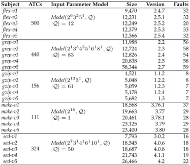
These subject programs have been widely used in test case prioritization research [4, 6, 13, 14, 29, 32–36]. Ta-ble 2 gives the program details, including the input pa-rameter model3, the number of ATCs obtained from the
Software-artifact Infrastructure Repository (SIR)4 [37], the program size excluding comments in lines of code (mea-sured by cloc5), the program version number, and the number of faults in each version. The ATC set for each
2. http://ftp.gnu.org/.
3. The input parameter model of each program was taken from the previous work by Petkeet al.[13, 14].
4. http://sir.unl.edu/. 5. http://cloc.sourceforge.net/.
TABLE 2 Subject Programs
Subject ATCs Input Parameter Model Size Version Faults
flex-v1 500 9,470 2.4.7 32 flex-v2 Model(263251,Q) 12,231 2.5.1 32 flex-v3 |Q|= 12 12,249 2.5.2 20 flex-v4 12,379 2.5.3 33 flex-v5 12,366 2.5.4 32 grep-v1 440 11,988 2.2 56 grep-v2 Model(213342516181,Q) 12,724 2.3 58 grep-v3 |Q|= 83 12,826 2.4 54 grep-v4 20,838 2.5 58 grep-v5 58,344 2.7 59 gzip-v1 156 4,521 1.1.2 8 gzip-v2 Model(21331,Q) 5,048 1.2.2 8 gzip-v3 |Q|= 61 5,059 1.2.3 7 gzip-v4 5,178 1.2.4 7 gzip-v5 5,682 1.3 7 make-v1 111 18,568 3.76.1 37 make-v2 Model(210,Q) 19,663 3.77 29 make-v3 |Q|= 1 20,461 3.78.1 28 make-v4 23,125 3.79 29 make-v5 23,400 3.80 28 sed-v1 324 7,793 3.0.2 16 sed-v2 Model(27314161101,Q) 18,545 4.0.6 18 sed-v3 |Q|= 50 18,687 4.0.8 18 sed-v4 21,743 4.1.1 19 sed-v5 26,466 4.2 22
TABLE 3
RSLCP,λLCP, ILCP, and SBP Techniques Considered in the Experiments
Category Mnemonic Description Prioritization Objective Reference
RSLCP
IV1 Pure 1-wise RSLCP-IV Covers the repeated maximum 1-wise level combinations Our study, and [17]
IV2 Pure 2-wise RSLCP-IV Covers the repeated maximum 2-wise level combinations Our study
IV3 (1 + 2)-wise RSLCP-IV Covers the independently-repeated maximum (1 + 2)-wise level combinations Our study
IV4 (2 + 1)-wise RSLCP-IV Covers the independently-repeated maximum (2 + 1)-wise level combinations Our study
IV5 Random Assignment RSLCP-IV Covers the independently-repeated maximum (1 or 2)-wise level combinations Our study
PV RSLCP-PV Covers the partially-independent-repeated maximum level combinations Our study
λLCP
1W LCP at prioritization strength 1 Covers the maximum 1-wise level combinations [30]
2W LCP at prioritization strength 2 Covers the maximum 2-wise level combinations [11]
3W LCP at prioritization strength 3 Covers the maximum 3-wise level combinations [11]
4W LCP at prioritization strength 4 Covers the maximum 4-wise level combinations [29]
5W LCP at prioritization strength 5 Covers the maximum 5-wise level combinations [31]
6W LCP at prioritization strength 6 Covers the maximum 6-wise level combinations [14]
ILCP ILCP Incremental-strength LCP Covers the maximum level combinations at incremental strengths [29]
SP GSPLSP Global SPLocal SP Achieves global maximum distanceAchieves local maximum distance [8][8]
program was constructed using the Test Specification Lan-guage (TSL) [38]. Apart from the programmake(for which some ATCs were removed due to unsuccessful execution), the ATCs used cover all valid level combinations at each strength.
4.3 The 15 Studied Prioritization Techniques
Table 3 gives an overview of the 15 prioritization techniques investigated, listing each technique’s category, mnemonic, description, prioritization objective, and corresponding ref-erence in the literature. Because RSLCP is a new version of LCP, we also considered anotherλLCP version, denotedλW, which we investigated for sixλvalues (λ= 1,2,3,4,5,6), following previous studies [6, 11, 14, 29–31]. In addition, we also compared our methods with another two widely-used ATCP techniques,Incremental-strength LCP(ILCP) [29], andSimilarity-based Prioritization(SP) [8]. ILCP makes use of incremental strengths beginning withλ= 1to runλLCP. We examined two versions of SBP [8],Global SP(GSP), andLocal SP(LSP): GSP initially selects two elements as the first two test cases with the minimum similarity, and then iteratively chooses an element as the next test case such that it has the minimum Jaccard similarity against previously selected test cases; LSP, in contrast, iteratively chooses a pair of test cases with the minimum Jaccard similarity until all candidates have been chosen [8].
4.4 Fault Seeding
For each of the subject programs, the original version con-tains no seeded-in faults. Although a number of hand-seeded faults are available from the SIR [37], many of these faults are easily detected (on average more than 60% of test cases can reveal them). In this study, therefore, we used mutation analysis [39] to seed in faults (see Table 2). As discussed in previous studies [40, 41], mutation analysis can provide more realistic faults than hand-seeding, and may be more appropriate for studying test case prioritiza-tion. Compared with real faults, however, the correlation between mutant killing ability and real fault detection may become weak when the test suite size is kept constant [42]. Nevertheless, the detection of real faults should improve significantly when test suites attain the highest levels of mutant kills [42]. In this study, each mutant could be killed by the given test suite.
For the five subject programs, we used the same muta-tion faults6as used by Henardet al.[35]. More specifically,
for each version Vi (1 ≤ i ≤ 5) of each subject program, the same mutant operators used in Andrews et al. [40] were adopted to produce the faulty versions (mutants) for our study. The operators used were: constant replacement; statement deletion; unary insertion; arithmetic operator re-placement; relational operator rere-placement; logical operator replacement; and bitwise logical operator replacement. As discussed by Henardet al. [35], equivalent7, and duplicated8
mutants were eliminated using the Trivial Compiler Equiva-lence (TCE) [44] tool, resulting in about one third of the mu-tants being removed. This was done to reduce interference
6. https://henard.net/research/regression/ICSE 2016/mutants/. 7. Equivalent mutants are functionally equivalent versions of the original program [43].
8. Duplicated mutants are equivalent to other mutants, but not to the original program [44].
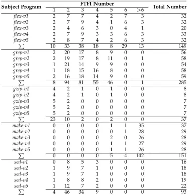
TABLE 4 FTFI Number Distribution
Subject Program 1 2 FTFI Number3 4 5 6 >6 Total Number
flex-v1 2 7 7 4 2 7 3 32 flex-v2 2 7 9 4 1 6 3 32 flex-v3 2 4 6 3 0 4 1 20 flex-v4 2 7 9 3 3 6 3 33 flex-v5∑ 2 8 7 4 2 6 3 32 10 33 38 18 8 29 13 149 grep-v1 2 20 17 8 9 0 0 56 grep-v2 2 19 17 8 11 0 1 58 grep-v3 1 21 14 9 9 0 0 54 grep-v4 1 18 15 16 8 0 0 58 grep-v5∑ 2 16 18 14 9 0 0 59 8 94 81 55 46 0 1 285 gzip-v1 4 2 1 0 1 0 0 8 gzip-v2 4 2 1 0 1 0 0 8 gzip-v3 5 2 0 0 0 0 0 7 gzip-v4 5 2 0 0 0 0 0 7 gzip-v5∑ 5 2 0 0 0 0 0 7 23 10 2 0 2 0 0 37 make-v1 0 0 0 0 1 1 35 37 make-v2 0 0 0 0 0 1 28 29 make-v3 0 0 0 0 2 0 26 28 make-v4 0 0 0 0 1 1 27 29 make-v5∑ 0 0 0 0 1 1 26 28 0 0 0 0 5 4 142 151 sed-v1 0 8 5 3 0 0 0 16 sed-v2 1 9 7 1 0 0 0 18 sed-v3 1 9 7 1 0 0 0 18 sed-v4 1 8 8 2 0 0 0 19 sed-v5∑ 1 12 7 2 0 0 0 22 4 46 34 9 0 0 0 93
in the fault detection evaluation of each prioritization tech-nique. Furthermore, as suggested by Papadakis et al. [45],
subsumed mutants [46] (also called disjoint mutants [47])9
were also identified and discarded [35] to avoid biasing the experimental results [43]. The subsumed mutants were removed by executing all ATCs for each mutant, and iden-tifying the failure-causing ATCs.
The performance of several ATCP techniques may de-pend on theFailure-Triggering Fault Interaction(FTFI) value of each mutant in each subject program, i.e., the number of parameters required to detect a failure [15, 48]. Table 4 shows the FTFI number distribution of each program.
4.5 Evaluation Metrics
In this study, we focused on the testing effectiveness and efficiency of RSLCP, from the perspectives of interaction coverage, fault detection, and prioritization cost.
4.5.1 Interaction Coverage Metric
The rate of interaction coverage was used to evaluate the speed of covering level combinations by the prioritized test suite. The Average Percentage of τ-wise Covering-array Coverage(APCC) [14], also calledAverage Percentage of Com-binatorial Coverage [27], was used to measure the rate of interaction coverage of strength τ achieved by prioritized ATCs. Its definition is given as follows:
Definition 4.1. Average Percentage of τ-wise Covering-array Coverage: Suppose S = ⟨t1, t2,· · · , tn⟩is a
prior-itized set of ATCs with size n, the APCC definition ofS at strengthτ (1≤τ≤k)is: APCC(τ, S) = ∑n i=1ψ(τ, ∪i j=1{tj}) n× |ψ(τ, S)| − 1 2n (11)
The APCC metric values range from 0.0 to 1.0, with higher values indicating better rates of interaction coverage at a specific strength τ. In this paper, following previous studies [14], we considered APCC withτ=1, 2, 3, 4, 5, and 6.
4.5.2 Fault Detection Metric
We used the fault detection rates of each prioritization technique as the fault detection metric. A well-known fit-ness function is the Average Percentage of Faults Detected
(APFD) [4], which measures the fault detection rate of a given prioritized test suite. Higher APFD values indicate better prioritized test sequences. The APFD is defined as follows:
Definition 4.2. Average Percentage of Faults Detected:
Suppose T is a test suite containingn test cases, andF is a set of m faults revealed by T. Let SFi be the number of
test cases in the prioritized test suiteSofTthat are executed before detecting fault fi. The APFD ofS is calculated using
the following equation (from Rothermel et al. [4]):
APFD(S) = 1−SF1+SF2+· · ·+SFm
n×m +
1
2n (12)
9. The mutants are subsumed or disjoint such that they are jointly killed when other mutants are killed.
4.5.3 Efficiency Metric
The prioritization cost measures how quickly each priori-tized test suite is constructed, and was used to represent the efficiency of the technique. Obviously, lower prioritization costs means better efficiency.
4.6 Inferential Statistical Analysis
Because some prioritization strategies involve randomiza-tion (due to the random tie-breaking technique [28]), we ran each experiment 1000 times, as suggested in previous studies [49].
As part of the investigation, we wanted to determine the statistical significance of any differences between the APCC or APFD values (used to evaluate each prioritization tech-nique), for which there are many statistical tests, such as the t-test and Wilcoxon-Mann-Whitney test [49]. Because there was no relationship among the 1000 iterations, we used an unpaired test [35]. Furthermore, because no assumptions were made about which prioritization technique was better than the other, a two-tailed test was used [35]. Following previous guidelines on inferential statistical approaches for dealing with randomized algorithms [49, 50], we used the unpaired two-tailed Wilcoxon-Mann-Whitney test to check the statistical significance (at a significance level of5%).
Since we used multiple statistical prioritization tech-niques, we report the p-values, which indicate whether or not the differences between two techniques are highly significant. When the p-value between two techniques M1
and M2 is less 5%, the difference between M1 and M2
is highly significant; otherwise, it is not significant. As Henard et al.[35] explained, however, with an increase of the number of the executions, p will become sufficiently small, which means that there are differences between two algorithms. However, when thep-value is very small, it may be difficult to identify which algorithm is actually the better. We therefore used a different statistical measure, the effect size, which is generally measured by the non-parametric Varia and Delay effect size measure [51],Aˆ12.
The Varia and Delay effect size measure should provide more useful information when comparing two different al-gorithms.Aˆ12(M1, M2) = 0.50, for example, would indicate
that in the sample, there is no difference between algorithms M1and M2.Aˆ12(M1, M2) > 0.50would mean thatM1 is
superior toM2; andAˆ12(M1, M2)<0.50would mean that M2is superior toM1. The further theAˆ12value is from 0.50,
the larger is the effect size. Based on previous work [51], we classify four categories of the effect size: no-difference (|Aˆ12(M1, M2)−0.50| = 0); small (0 < |Aˆ12(M1, M2)−
0.50| ≤ 0.10); medium (0.10 < |Aˆ12(M1, M2)−0.50| ≤
0.17); and large (|Aˆ12(M1, M2)−0.50|>0.17).
5
R
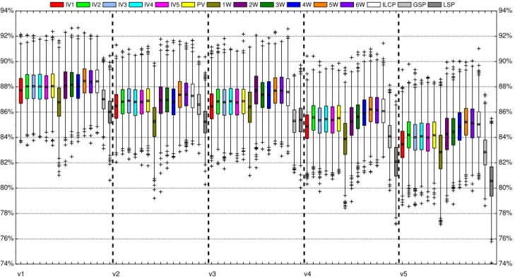
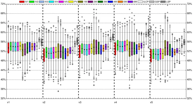
ESULTSThis section presents the results of the experiments conduct-ed, and answers the research questions. In the displayed results, each box plot shows the distribution of the 1000 APCCs or APFDs (averaged over 1000 iterations), listed horizontally across the figure. Each box plot shows the mean (square in the box), median (line in the box), upper and lower quartiles, and minimum and maximum APCC
values for the prioritization technique. In addition, a sta-tistical analysis is given for each pairwise APCC or APFD comparison of prioritization techniques. For example, for a comparison between two methodsM1 vsM2, we usem to
denote that there is no statistical difference between them (i.e., theirp-value is greater than 0.05);4to denote thatM1
is significantly better (p-value is less than 0.05, and the effect size Aˆ12(M1, M2) is greater than 0.50); and 6 to denote
thatM2is significantly better (p-value is less than 0.05, and
ˆ
A12(M1, M2)is less than 0.50). 5.1 Interaction Coverage Results
In this section, we answer RQ1,RQ2, and RQ3, from the perspective of the interaction coverage rates. Figures 3 to 7 present the APCC results for programsflex,grep,gzip,make, andsed. Each figure describes different strength values for APCC, i.e., τ is assigned 1, 2, 3, 4, 5, and 6. Tables 5 and 6 show the detailed Wilcoxon test APCC results at the 0.05 significance level for each comparison.
5.1.1 RQ1: RSLCP Techniques
Here, we try to answer the sub-questions of RQ1: RQ1.1
and RQ1.2, according to APCC, and then briefly analyze each observation.
(1)RQ1.1: RSLCP-IV Techniques:Based on the experimen-tal results, we can observe the following:s
• When τ = 1, all RSLCP-IV techniques have very similar APCCs for all programs, because their 1-wise APCCs have very similar distributions. According to the statistical analysis (Table 5), however, IV1 and IV3 generally have the best performances, followed by IV5, regardless of subject programs (apart from programsgzipandmake).
• When2≤τ≤6, it can be observed that IV2 overall has the best performance for all programs, followed by IV4; while IV1 is worst, followed by IV5 and IV3. The statistical analysis (Table 5) also confirms these observations.
The main reason for the first observation is that both IV1 and IV3 initially make use of λ = 1 for prioritizing ATCs, which is the same mechanism as 1W — 1W chooses an element as the next test case such that it covers the largest number of 1-wise level combination that have not been covered by previously selected ATCs. When all 1-wise level combinations have been covered by the selected ATCs, the order of the remaining ATCs does not change the 1-wise APCC value. Therefore, IV1 and IV3 perform very similarly, and have better 1-wise APCCs than other RSLCP-IV techniques. Regarding the difference for programsgzip
andmake, a possible reason may be that an element covering the largest number of uncovered 2-wise level combination-s (combination-selected acombination-s the next tecombination-st cacombination-se by IV2, IV4, and IV5), could cover a comparable number of uncovered 1-wise level combinations as IV1 and IV3, due to the characteristics of the input parameter model (i.e., each parameter contains a similar number of levels).
The second observation can be explained as follows: Similar to the case of IV1 and IV3, IV2 and IV4 have the same APCC values at τ = 2. However, IV2 repeatedly covers entire 2-wise level combinations, which may provide the faster speed to cover level combinationsτ >2than other RSLCP-IV techniques. Similarly, IV1 only repeatedly covers entire 1-wise level combinations, which may not provide higher rates of interaction coverage at higher strengths.
From the perspective of the interaction coverage rate, the answer toRQ1.1 is: Overall, IV2 has the best performance among all RSLCP-IV techniques, followed by IV4; and IV1 is generally the worst.
(2)RQ1.2: RSLCP-IV vs RSLCP-PV:Based on the experi-mental data, we have the following observations:
• Whenτ = 1, PV has very similar APCC values to RSLCP-IV techniques for all programs. Apart from programsgzipandmake, however, the statistical anal-ysis shows that compared with IV1 and IV3, there is no highly significant difference compared with PV; while the difference between PV and IV2, IV4, or
97.0 97.2 97.4 97.6 97.8 98.0 98.2 98.4 98.6 98.8 99.0 99.2 99.4 99.6 99.8 6W 5W 4W 3W 2W 1W PV ILCPGSPLSP IV5 IV4 IV3 IV2 IV1 A P C C ( % ) (a)τ= 1 93.5 94.0 94.5 95.0 95.5 96.0 96.5 97.0 97.5 98.0 98.5 99.0 99.5 6W 5W 4W 3W 2W 1W PV ILCPGSPLSP IV5 IV4 IV3 IV2 IV1 A P C C ( % ) (b)τ= 2 90.5 91.0 91.5 92.0 92.5 93.0 93.5 94.0 94.5 95.0 95.5 96.0 96.5 97.0 97.5 98.0 6W 5W 4W 3W 2W 1W PV ILCPGSPLSP IV5 IV4 IV3 IV2 IV1 A P C C ( % ) (c)τ= 3 87 88 89 90 91 92 93 94 95 96 6W 5W 4W 3W 2W 1W PV ILCPGSPLSP IV5 IV4 IV3 IV2 IV1 A P C C ( % ) (d)τ= 4 82 83 84 85 86 87 88 89 90 91 92 6W 5W 4W 3W 2W 1W PV ILCPGSPLSP IV5 IV4 IV3 IV2 IV1 A P C C ( % ) (e)τ= 5 75 76 77 78 79 80 81 82 83 84 85 86 6W 5W 4W 3W 2W 1W PV ILCPGSPLSP IV5 IV4 IV3 IV2 IV1 A P C C ( % ) (f)τ= 6
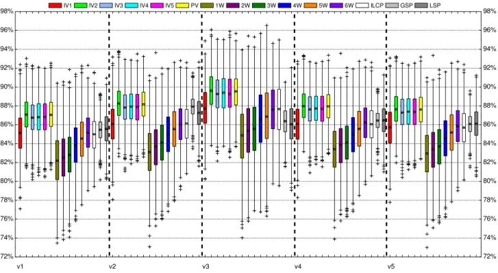
96.8 97.0 97.2 97.4 97.6 97.8 98.0 98.2 98.4 98.6 98.8 99.0 99.2 99.4 6W 5W 4W 3W 2W 1W PV ILCPGSPLSP IV5 IV4 IV3 IV2 IV1 A P C C ( % ) (a)τ= 1 92.0 92.5 93.0 93.5 94.0 94.5 95.0 95.5 96.0 96.5 97.0 97.5 98.0 6W 5W 4W 3W 2W 1W PV ILCPGSPLSP IV5 IV4 IV3 IV2 IV1 A P C C ( % ) (b)τ= 2 85 86 87 88 89 90 91 92 93 94 95 6W 5W 4W 3W 2W 1W PV ILCPGSPLSP IV5 IV4 IV3 IV2 IV1 A P C C ( % ) (c)τ= 3 78 79 80 81 82 83 84 85 86 87 88 89 6W 5W 4W 3W 2W 1W PV ILCPGSPLSP IV5 IV4 IV3 IV2 IV1 A P C C ( % ) (d)τ= 4 72 73 74 75 76 77 78 79 80 81 82 6W 5W 4W 3W 2W V 1W 5 P ILCP GSP LSP 4 IV 3 IV 2 IV 1 IV IV A P C C ( % ) (e)τ= 5 66 67 68 69 70 71 72 73 74 75 6W 5W 4W 3W 2W V 1W 5 P ILCP G LSP 4 IV 3 IV 2 IV 1 IV IV A P C C ( % ) SP (f)τ= 6
Fig. 4. APCC results for each prioritization technique for the programgrep.
96.6 96.8 97.0 97.2 97.4 97.6 97.8 98.0 98.2 98.4 98.6 98.8 6W 5W 4W 3W 2W 1W PV ILCPGSPLSP IV5 IV4 IV3 IV2 IV1 A P C C ( % ) (a)τ= 1 93.6 94.0 94.4 94.8 95.2 95.6 96.0 96.4 96.8 97.2 97.6 6W 5W 4W 3W 2W 1W PV ILCPGSPLSP IV5 IV4 IV3 IV2 IV1 A P C C ( % ) (b)τ= 2 90.0 90.5 91.0 91.5 92.0 92.5 93.0 93.5 94.0 94.5 95.0 95.5 6W 5W 4W 3W 2W 1W PV ILCPGSPLSP IV5 IV4 IV3 IV2 IV1 A P C C ( % ) (c)τ= 3 87.0 87.5 88.0 88.5 89.0 89.5 90.0 90.5 91.0 91.5 92.0 92.5 93.0 6W 5W 4W 3W 2W 1W PV ILCPGSPLSP IV5 IV4 IV3 IV2 IV1 A P C C ( % ) (d)τ= 4 82.5 83.0 83.5 84.0 84.5 85.0 85.5 86.0 86.5 87.0 87.5 88.0 88.5 89.0 89.5 6W 5W 4W 3W 2W 1W PV ILCPGSPLSP IV5 IV4 IV3 IV2 IV1 A P C C ( % ) (e)τ= 5 78.0 78.5 79.0 79.5 80.0 80.5 81.0 81.5 82.0 82.5 83.0 83.5 84.0 84.5 85.0 85.5 86.0 6W 5W 4W 3W 2W 1W PV ILCPGSPLSP IV5 IV4 IV3 IV2 IV1 A P C C ( % ) (f)τ= 6
Fig. 5. APCC results for each prioritization technique for the programgzip.
IV5 is highly significant. In addition, the statistical analysis also shows that PV is similar to IV1 and IV3, but performs better than other RSLCP-IV techniques whenτ= 1.
• When 2 ≤ τ ≤ 6, PV is worse than IV2 for all programs, but performs better than IV1, IV3, and IV5. The statistical analysis confirms the box plot observations. PV has comparable APCC values to IV4. However, the statistical analysis shows that IV4 has significantly better 2-wise APCCs than PV; but for highτ values, the opposite is true: PV has signif-icantly betterτ-wise APCCs than IV4.
A plausible reason to the first observation is that, as was the case for IV1 and IV3, PV uses 1W at the start of the prioritization process, which guarantees that it has similar speeds to IV1 and IV3, but higher speeds than other RSLCP-IV techniques for covering 1-wise level
combina-tions. However, IV2 uses 2W to prioritize ATCs, while PV uses 1W and 2W to guide the prioritization. Therefore, IV2 may provide faster speeds than PV for covering high τ value level combinations. Similarly, IV4 initially uses 2W for prioritizing ATCs, and then independently chooses 1W to prioritize the remaining ATCs when 2-wise level combi-nations have been fully covered. This process may provide better 2-wise APCCs than PV. However, when all 1-wise level combinations have been covered by the selected ATCs, PV does not independently use 2W for prioritizing the remaining ATCs, i.e., it considers 2-wise level combinations that have not yet been covered by previously selected ATCs (obtained by 1W). This process may guarantee that PV has higher APCCs than IV4.
With respect to the interaction coverage rate, the answer toRQ1.2is: Overall, PV achieves a better performance than other RSLCP-IV techniques.