Using Classification for Analysis of Multi-Modal Video Summarization

(1)

Rochester Institute of Technology Rochester Institute of Technology

RIT Scholar Works

Theses

8-2020

Using Classification for Analysis of Multi-Modal Video

Summarization

Brendan Wells

[email protected]

Follow this and additional works at: https://scholarworks.rit.edu/theses

Recommended Citation Recommended Citation

Wells, Brendan, "Using Classification for Analysis of Multi-Modal Video Summarization" (2020). Thesis. Rochester Institute of Technology. Accessed from

This Thesis is brought to you for free and open access by RIT Scholar Works. It has been accepted for inclusion in Theses by an authorized administrator of RIT Scholar Works. For more information, please contact

(2)

Using Classification for Analysis of Multi-Modal

Video Summarization

(3)

Using Classification for Analysis of Multi-Modal

Video Summarization

Brendan Wells August 2020 A Thesis Submitted in Partial Fulfillment

of the Requirements for the Degree of Master of Science

in

Computer Engineering

COE_hor_k https://www.rit.edu/engineering/DrupalFiles/images/site-lockup.svg

1 of 1 1/9/2020, 10:42 AM

(4)

Using Classification for Analysis of Multi-Modal

Video Summarization

Brendan Wells

Committee Approval:

Dr. Alexander LouiAdvisor Date

Department of Computer Engineering

Dr. Corey Merkel Date

Department of Computer Engineering

Dr. Andres Kwasinski Date

(5)

Acknowledgments

Thank You to My Advisor Dr.Loui for helping me along the Research Process. Thank You to My Committee of Dr.Kwasinski and Dr.Merkel for helping Oversee the Research Process and Provide me with Valuable Feedback.

Thank You to the Computer Engineering Department at Rochester Institute of Tech-nology for Teaching me the Skills to Conduct this Research.

Thank You to Research Computing at Rochester Institute of Technology for Providing me the Resources to Conduct this Research.

(6)

This research is dedicated to my family, friends, teachers, and mentors along the way who pushed me to always take the next step.

(7)

Abstract

Video Summarization refers to taking the important contents of a video and condens-ing it down to an easily consumable piece of data without havcondens-ing to watch the entire video. Currently, Millions of Videos are being recorded and shared every day. These videos range from the consumer level, such as a birthday party or wedding video, all the way up to industry such as film and television. We have constructed a model that seeks to address the problem of not being able to consume all the media that is being presented to you because of time constraints. To do this, we conduct two separate experiments. The first experiment examines the role of different parts of the summarization model, namely modality, sampling rate, and data scaling so that we better understand how summaries are generated. The second experiment utilizes these findings to create a model based in classification. We use classification as a means of interpreting a wide variety of types of video for summarization. By using classification to generate the video and audio features used by the summarizer, the classifier granularity is leveraged, and the maturity of classification problems is lever-aged to accomplish a summarization task. We found that while scaling and sampling of the data have little effect on the overall summary, in each experiment the modality played a large role in the results. While many models exclude audio, we found that there are benefits to including this data when generating a video summary. We also found that the use of classification resulted in a separation of impacts for each modal-ity, with video serving to construct the shape of the summary and audio determining importance score.

(8)

List of Figures

3.1 Modality Comparison Model . . . 11

3.2 VGG-Based model used in Modality Analysis . . . 11

3.3 Pre-Fusion Summarization Model with Classification . . . 13

3.4 Post-Fusion Summarization Model with Classification . . . 14

4.1 Example Output with both Expectation and Prediction scoring Shown 20 5.1 Scaling Accuracy and Loss Results . . . 23

5.2 Interval Accuracy and Loss Results . . . 24

5.3 Modality Accuracy and Loss Results . . . 24

5.4 TVSum Example 1 . . . 27

5.5 TVSum Examples 2 & 3 . . . 28

5.6 Scaling Accuracy and Loss Results . . . 29

5.7 Interval Accuracy and Loss Results . . . 29

5.8 Modality Accuracy and Loss Results . . . 30

5.9 SumMe Example 1 . . . 31

5.10 Sume Examples 2 & 3 . . . 32

5.11 Video Accuracy Results . . . 33

5.12 Video Loss Results . . . 33

5.13 Video Average Results . . . 34

5.14 Audio Accuracy Results . . . 35

5.15 Audio Loss Results . . . 35

5.16 Audio Average Results . . . 36

5.17 Combined Accuracy Results . . . 36

5.18 Combined Loss Results . . . 37

5.19 Combined Average Results . . . 37

5.20 TVSum Example Output 1 . . . 41

5.22 TVSum Example Output 2, Scores of 3 or above . . . 43

5.24 Video Accuracy Results . . . 46

5.25 Video Loss Results . . . 46

5.26 Video Average Results . . . 47

(11)

LIST OF FIGURES

5.28 Audio Loss Results . . . 48

5.29 Audio Average Results . . . 48

5.30 Combined Accuracy Results . . . 49

5.31 Combined Loss Results . . . 49

5.32 Combined Average Results . . . 50

5.33 SumMe Example Output 1 . . . 52

(12)

List of Tables

3.1 Dense Network Comparison . . . 15

4.1 TVSum Video Cateogries . . . 19

5.1 F-Scores for TVSum Categories . . . 26

5.2 F-Scores for Dense-2 and Dense-4 for TVSum . . . 40

5.3 F-Scores for Dense-2 Post-Fusion on TVSum . . . 45

(13)

Chapter 1

Introduction

In the world today, video is being recorded everywhere for many different reasons. Millions of hours of video are recorded everyday, with sites like Youtube announcing that over 500 hours of video is uploaded every minute. These videos range from home videos like those of a birthday party or special event, to video that is always being captured like a security camera or self-driving car cameras. Between the amount of video that we see on television, social media, or anywhere else, it is impossible to watch everything that is being presented to us on a daily basis. One solution that arises to solve this problem is to instead watch a summary of the important moments of videos.

Video Summarization refers to the process of taking a video and creating a sum-mary of it based on its important parts. The goal of Video Summarization is that the resulting summary saves the user time by not having to watch the entire video to get a basic understanding of its content. The form that these summaries take varies between implementations. The summary method that we will be focusing for our implementation is known as a keyshot summary [1, 2, 3, 4, 5]. In a keyshot summary, multiple sub-clips are selected so that the output is a short set of highlighted moments from throughout the video. The sub-clips form a much shorter video than the original that can be watched in a fraction of the time. An important element of creating this video summary is the source video. In this work we focus on multi-modal data

(14)

mean-CHAPTER 1. INTRODUCTION

ing both the audio and the video from a video will be analyzed. Some approaches focus solely on the video aspect and do not use the audio data [1, 2, 3].

In the following chapters, we will both analyze different approaches to Video Summarization, as well as propose our own method that has shown potential to form meaningful summaries. In Chapter 2, we discuss a brief history of Video Summariza-tion, including different methods, types of summaries, and where the current state of the art stands. In Chapter 3, we discuss our how we analyzed the effects of multi-modal data on video summaries, as well as our proposed method for summarization base on these results. Chapter 4 discuss how the experiments were conducted and the data that was used. Chapters 5 & 6 include the results of our experiments and our analysis of those results, as well as the conclusions we can draw from these ex-periments and outline future work that stands to build on our results.

Throughout these chapters, we hope to focus on two main points. The first point of focus was analyzing how the multi-modal nature of the input video affects the final summary. The second point of focus was finding a way to use the results from the the first point to improve how summaries are being generated. Specifically, we choose to leverage classification techniques to make use of these results and improve our summaries.

(15)

Chapter 2

Background

2.1 Video Summarization before Deep learning

Video Summarization is a task that has been studied long before deep learning came to be popular. Even in the early 1990’s, there were studies being conducted on how best to summarize consumer video. In 1991 Microsoft Research published research about several early techniques they had evaluated to create video summaries [6]. The algorithms they were testing were based on specific statistical properties of the videos, such as pitch activity in the audio, transitions of the video feed, or user activity and how people interacted with the video itself. Their output in this study was a keyshot summary, with their goal being 20-25% of the original video length for that summary. For a metric of quality, they used two main factors. They quizzed the participants on knowledge of the video, as well as conducted a survey of the summary asking for a rating of different categories, including clarity and conciseness of the summary. Until the popularization of deep learning around 2012, video summarization continued to use these types of methods. Over time, different improvements and enhancements were made to the video summarization process. One study used Singular Value Decomposition to analyze videos and generate their keyframes that way [7]. This method focused specifically on identifying the emotions of speech combined with a high amount of visual action. Another study specifically examined home video. This

(16)

CHAPTER 2. BACKGROUND

study focused on creating algorithms that utilized the circumstances of the video as part of their summarization process [8]. They used the time and date the video was taken as part of the processing. This was done by creating several cluster categories based on how the data was related, such as continuous activities being one cluster, and all events from a single day being another.

In 2011, a group from Kodak Research was investigating video summarization specifically with consumer video [9]. They first split the video and audio into separate modalities to summarize. Their audio summarization method involved segmenting audio clips using a sliding algorithm to create segments at reasonable boundaries. From there, they classified the clips into specific types that they were analyzing, such as singing or speech. The audio was processed into several different feature groups and then used to train a Support Vector Machine, or SVM, classifier for each of the chosen audio classes. A K-means clustering algorithm was then created that used the detection scores of the audio to determine how important the audio was to the summary. For the video data, keyframes were selected using a variety of criteria including quality of the image, quality of faces detected in the image, and diversity among the keyframes. This work is of particular note because the process that we used in our model follows a similar data flow. It also is much more recent than the earlier methods, and while still not deep learning based, does use machine learning elements such as SVM classifiers and a k-means clustering algorithm.

One common factor of video summarization throughout this time was that the results were typically judged based on quizzes or surveys of people after the fact. There were common themes among these quizzes, such as asking the participants how they felt about clarity of summary, or how concise it was compared to the original. This is one of the elements of the video summarization process that we see continue through to today. Summary ground truths currently are still subjective, with groups of participants answering their opinion of a video. Although the categories and how

(17)

this rating is found has changed overtime, it is important to note that even after 30 years the same subjective process is required for video summarization.

2.2 Applying Deep Learning Techniques

With the introduction of AlexNet [10] in 2012, deep learning techniques became an increasingly popular method for solving complex problems. This includes video sum-marization. One early example from 2015[11] of the use of deep learning for video summarization doesn’t utilize these techniques for the summarization, but rather as an objective that is used to evaluate the summary. They specifically used a classifi-cation network called DeCAF[12] to compare object classes as a way to evaluate how representative of the original video the summary was. However, their summariza-tion model was still algorithmic like previous approaches rather than based in deep learning.

One of the earlier models to fully implement deep learning was based on a Long Short-term Memory approach, and was called vsLSTM.[1] They used their model to generate keyshot summaries similarly to what we propose. These LSTM based mod-els have become popular for video summarization tasks because they can make use of temporal information compared to other deep learning models. Another LSTM based model from 2017 focused on unsupervised learning with a diversity & representative-ness reward system [13]. This model is an encoder-decoder model that uses a CNN encoder and an LSTM decoder. A reward function then checks the results based on how diverse it is to make sure a variety of clips are chosen, as well as a representative-ness score to make sure it is a quality summary. Unsupervised models benefit in the fact that they can potentially learn from more videos than supervised models. This solves one of the major problems that video summarization models struggle from with a lack of datasets, as mentioned previously. An separate unsupervised model again from 2017 used an LSTM, but in this case specifically was an adversarial LSTM

(18)

net-CHAPTER 2. BACKGROUND

work. This model featured multiple sub-LSTM networks that created an adversarial network that took input from a summarizer LSTM. Not every video summarization model based in deep learning is an LSTM model though. One approach from 2018 used a fully convolutional sequence network to accomplish the task.[3] This model used a convolutional neural network to try to summarize videos. Specifically, they chose to use FCN [14] which is known for being a semantic segmentation network to accomplish this task. They presented both supervised and unsupervised models for accomplishing this. An important note is that these models all focused on the video data, and not on the audio. Many models fall into this category of not using the audio features when creating their summaries. Some models do use both however. One model for video classification rather than summarization utilized a mix of CNNs and LSTMs, spanning both video and audio to classify videos into categories.[15] So although not a summarization model, they apply a similar technique to what we are attempting by using both the video and audio data.

2.3 State of the Art

One model, called AENet[16] specifically focused on audio data as a means of aug-menting current state of the art. They proposed that by augaug-menting current video models with an audio model, they could achieve more accurate results than a video model on its own. Using both the video and audio data, they achieved an overall accuracy of 80.3% without data augmentation and a 56.6% mean average precision score. This was tested on their own dataset that used 100 videos from youtube. This was published in 2018 and to the best of our knowledge is state of the art for models using both video and audio data.

To the best of our knowledge, the State of the Art model when only using video is a supervised LSTM. This model, biLSTM [2], utilizes an encoder-decoder basis, where the encoder is a bidirectional LSTM model, and the decoder uses an attention

(19)

mechanism to generate the output. The purpose of the encoder is to first extract the context during the bidirectional LSTM, meaning that a sequence is both analyzed forwards and backwards, and then simplified. The decoder then takes the information and uses an attention model to determine the important information that remains following the encoding process. Their results are currently state-of-the-art, reaching an F-Score of 44.4 on SumMe and 61.0 on TVSum without data augmentation. An important note is that their model ignores audio features.

(20)

Chapter 3

Approach

3.1 Ideology

For our experiments, we wanted to focus specifically on creating keyshot summaries. This approach has a wide variety of applications, as well as has a large room for im-provement. This stems from the fact that keyshot summaries are particularly difficult to create. This comes from two main factors. The first one is that a keyshot sum-mary is subjective. The goal of a keyshot sumsum-mary is to capture the most important points of a video to create a shorter video that still captures the main points of the original. This will vary from person to person, making a perfect summary difficult to achieve. This is compared to other types of summaries such as a caption or text based summary. These text based summaries typically identify the general events of the video. These have much more of a factual basis as someone can objectively say the events summarized either happened in the video, or they did not. Keyshot summaries unfortunately aren’t as simple as this because of the subjective nature of importance rankings, which results in the difficulty to produce a summary. The second reason that creating keyshot summaries is difficult is related to their subjec-tivity, in the factor that there is limited datasets for keyshot summarization available. Although there are many video datasets that exist, there are few that are focused on summarization. Most video summarization research relies heavily on two main

(21)

CHAPTER 3. APPROACH

datasets, being TVSum [17] and SumMe [18]. The specifics of these datasets are covered in chapter 4. These datasets are widely used for creating keyshot summaries due to their frame level importance scoring, but they only examine 75 total videos between the two. Despite the difficulty in keyshot summaries, there is a wide variety of applications that they can be used for. One of the simple applications could be home videos being uploaded and shared to social media for others to watch. With how much media is shared online, this can save people time while still sharing their stories and memories. Another application could be for industry application, like creating a highlight from a sports game or a trailer for a movie that can then be shared. One application that can make use of both the video and audio specifically is in a security application. In the example of a home security camera placed in a door way, sound can play an important role in creating a summary. For a security application, these types of videos could be taken using a recorder that is always on. This means large blocks of similar video is analyzed. If a large noise is heard off camera around the side of the house, that is incredibly important to generating an accurate summary of what happened and when it happened. These applications are why we believe keyshot summaries are important, and also why we believe the audio data can be leveraged in summarization applications.

3.2 Modality Analysis

For the first point of focus, we wanted to examine how using both the visual and audio data from the input video affected the resulting summary. Specifically, we wanted to examine the three different scenarios of using only the video, only the audio, and using both to create an output summary.

To create an accurate comparison, the same model was used to test all three cases, with the exception of the input layer size being doubled for the CNN using both video and audio. The flow model is shown in Figure 3.1.

(22)

CHAPTER 3. APPROACH

Figure 3.1: Modality Comparison Model

The CNN used in the model was a variation on the popular VGG16 [19]. VGG was chosen due to its flexibility across machine learning applications, specifically with image and audio processing as well as its simplicity. This CNN is shown in Figure 3.2.

Figure 3.2: VGG-Based model used in Modality Analysis

To get a better understanding of how the input data affects the summary, we examined several other factors within this experiment. The first one was the scaling of the input data. Scaling input data is a popular method in machine learning to reduce computations. We wanted to see how this operation might have an effect on the resulting summary. The second factor we wanted to examine was the sampling rate of the data. With the summarization model having to sample the video, the sampling rate becomes an important factor in how a summary is generated. Several sampling rates for the videos were chosen to test if changing this value had an effect.

(23)

CHAPTER 3. APPROACH

3.3 Summarization through Classification

For our approach to creating a keyshot summary, we wanted to focus on the two main problems outlined previously. To help with the lack of data, we decided that we will use both sources of data. This was also influenced by the results of the previous experiment mentioned. To address the difficulty of summarization, we decided to simplify the problem by offloading part of the summarization. To do this, we leveraged a previous machine learning problem of classification. We believe that by classifying the data before creating a summary, you generalize the subject points upon which the summary is created. Logically, we believe this reflects how a human would summarize a video. Typically the importance of the video is based on the main subject points, rather than the background. The classifier reflects this. Using the home security camera example, the important parts of the video may be the appearance of a person with a package. These classes are identified and when combined are recognized as important. For a birthday party video, the same could be said when both the classes for a cake and singing appear at the same point.

We also believe that this approach will help with generalizing the model while still working with a limited amount of data. With the amount of variation in videos, classification will serve to simplify the problem to be based on class relationships rather than the raw data. These class relationships serve to generalize problems based on classifier granularity. If the classifier has general balloon and cake classes, then any type of video containing these objects can be summarized. By learning based on the confidence of the classes, the event itself is generalized. Instead of having to learn how to summarize a graduation party, compared to birthday party or retirement party, the events become simplified by their key classes. As the classifiers become more powerful, so to will the summary and the types of video that can be summarized. This allows for the summarization model to improve without requiring

(24)

CHAPTER 3. APPROACH

additional data, which addresses one key problem of keyshot summarization.

3.3.1 Pre-Fusion Classification Model

The first model constructed is a pre-fusion model for the classification. This approach follows the same design path as the comparison model from the previous experiment, except instead of combining the raw data, it is the class predictions that are combined into a class-prediction vector. For this model, the class predictions are concatenated into one longer vector conatining both the video and the audio classes. Rather than combine similar audio and video classes, we choose to keep them separate as the audio and video aspects of matching classes may have different contexts which would be loss when combined. This class prediction vector is what is then input into a single summarizer, which then performs a single summarization. With there only being a single summarization, this model learns both the video and audio aspects simultaneously. This matches with the dataset ground truth that was used where a single ground truth value is assigned per frame. The ground truths were not created separately for the video and audio, so this distinction is important for the creation of the summary. For the summarizer itself, with the input being a vector of class predictions we chose to use a dense network. This model is presented in Figure 3.3. The specific parameters used in configuring the models for both the summarizer and classifier are discussed in chapter 4.

(25)

CHAPTER 3. APPROACH

3.3.2 Post-Fusion Classification Model

The second model constructed is a post-fusion model for the classification. This model is similar to the pre-fusion model, except two separate summarizations are performed instead, with the results being combined after. This allows for flexibility in the model with with weighting being possible towards one type of data. Again, a class-prediction vector is created with the classifiers, but separate dense networks are used to create the final summary values. The one notable point here is that with two summarizers, the audio and video become weighted separately using a single ground truth. With the datasets having a general scoring of importance, it is not possible to separate them. This leads to cases of the video being important with no audio importance yet both summarizers learning that frame was important. To combine the predictions of each model, the predictions are averaged and then a floor function is applied to them. This results in even weighting for this model, however weighting each modality differently is an option that warrants future research. The model is presented in Figure 3.4. The specific parameters used in configuring the models for both the summarizer and classifier are discussed in chapter 4.

Figure 3.4: Post-Fusion Summarization Model with Classification

3.3.3 Summarization Dense Networks

While the Post-Fusion and Pre-Fusion Models illustrate the overall flow of the data processing, the dense network that is used to perform the summarization part of the model requires a more in-depth analysis. This network was responsible for taking the

(26)

CHAPTER 3. APPROACH

class predictions from the classifier and converting those into the summary results. In total, 7 different dense networks were created and tested using different configura-tions of layers and optimizaconfigura-tions. This was done because whereas we have a general understanding of how different optimizations affect raw data, such as batch normal-ization [20] and dropout [21], we don’t have the same data for our class prediction matrix. This is reflected with the different networks that were created. The different configurations can be seen in Table 3.1.

Table 3.1: Dense Network Comparison

Name # Layers # Nodes Activation? Batch Norm? Dropout?

Dense-1 3 16 No No No

Dense-2 3 16 Yes Yes Yes

Dense-4 3 16 Yes No No

Dense-5 3 16 Yes Yes No

Dense-7 6 16 (1,2) / 8 (3,4,5) Yes No No

For every network configurations, there were some common factors. The number of layers includes both the input and final output layer. The final output layer was always a dense layer of 5 classes, followed by a softmax operation. The activation column refers to activation functions between layers. If the configuration had activa-tion funcactiva-tions, it was always ReLu [22]. For dropout layers, the dropout was always set to 50%.

One important aspect of our approach is the use of a dense network as the sum-marizer. We do acknowledge that by using a dense network, the temporal context is lost in this approach. When using an LSTM model like state-of-the-art models do, this context is retained. For our model, we believe the dense network configuration

(27)

CHAPTER 3. APPROACH

is a better choice for two reasons. The first is that with the class prediction vector that is generated as described previously, a dense network can fully process that data structure as it is fairly simple. This allows for those class relationships that we de-scribed to be formed. The second reason that the dense network is better is because without the temporal context, class relationships become cross video. This means if a class represents high importance in one video, that is the truth across all videos. In a temporal context, a class may only be important due to showing up for an extended period of time in a video. However if the class is inherently important, it can be related to in all contexts without a temporal dependence. For example, if a firetruck visual class is learned to be a 5 importance, summaries that contain that class will always reach a score of 5 importance. If another summary doesn’t contain that class, and no other class scores a 5 importance, the summary will have a maximum score of less than 5. In certain applications, these scores can be used to compare a summary or judge a video. If a video has summary that reaches a 5 compared to one that doesn’t, one video may be deemed more important or of higher interest.

(28)

Chapter 4

Experiments

4.1 Data Extraction

Before training, both the audio and visual data were extracted from the videos sep-arately. For the visual data, each video was separated into individual image frames that could input into the model. The audio data was split into short audio samples. The time of the audio samples matched the sampling rate of the selected video frames. For example, in a video with 30 frames per second and a desired sampling of every second, every 30th image frame and 1 second of audio would be used. The audio starts on the sampled frame, so in a case of frame 0, the audio would correspond to the audio heard during frames 0-29. The sampling rate of the data was variable depending on the experiment, as this was one of the parameters examined in the testing.

4.2 Data Processing

Once the data was extracted from each video it was pre-processed. The pre-processing depended on which experiment was being conducted.

(29)

CHAPTER 4. EXPERIMENTS

4.2.1 Modality Comparison Experiment

The first experiment focused on how audio and visual data produce separate sum-maries and how they interact with each other. For this, the main focus of the tests was different ways of tuning the pre-processed data. For the visual data, different image sizes were experimented with to examine how downsizing the data had an ef-fect on the summary. This process consisted of first resizing every image to 224x224. This was picked as it is the common size used for image processing in deep learning models. This was considered to be the full scale images for testing. From there, the images were also resized down to 112x112 and 56x56 for corresponding tests at half and quarter scale. For the audio data, in this experiment each audio sample was taken and the MFCC’s were calculated over the duration of the sample. For the model that used both the audio and the video, the data was also concatenated to create a matrix with twice the height of the visual data, with the visual data being the upper half of the matrix and the audio data being the lower half. The reasoning behind this method was that neither data had more representation in the input, and therefore would not bias the result towards a specific type of data. This was an important factor for when the results were compared.

4.2.2 Classification Experiment

The second experiment that focused on our proposed method of summarization using classification required a different pre-processing than the previous experiment. Both data sources were input into classifiers to develop a class matrix that would instead be input into the summarization model. For the visual data, the images were each input into a VGG16 pre-trained ImageNet classifier [19]. This classifier was chosen as it is one of the most popular image classifiers, has high performance, and has a wide variety of classes. This specific classifier used 1000 classes from ImageNet. For the Audio data, the pre-trained Yamnet Model [23] was used. This classifier is trained

(30)

Table 4.1: TVSum Video Cateogries

Abbreivation Category

VT Changing Vehicle Tire VU Getting Vehicle Unstuck GA Grooming an Animal MS Making Sandwich

PK Parkour

PR Parade

FM Flash Mob Gathering BK Bee Keeping BT Attempting Bike Tricks

DS Dog Show

on the Audioset dataset [24] and featured 521 different audio classes. The output of the classifiers were an array of predictions for each class. Based on the result of the previous experiment, a sampling rate equal of 1 second was chosen when selecting images and creating audio clips for the classifiers.

4.3 Datasets

The first dataset used was the TVSum dataset [17]. This dataset has 50 Youtube videos from 10 different categories with 50 Human summaries each. The videos have labels of importance ranking from 1-5, with 1 scoring as the least important and a 5 meaning most important.Importance for this ground truth was determined by people determining how important the segment is in relation to the overall video. The categories for the TVSum dataset are shown in Table ??.

The Second Dataset that will be used is the SumMe dataset [18]. This along with TVSum are the main datasets used for video summarization experiments. This dataset has 25 videos, each containing 15 human summaries. 2 of these videos were omitted from our experiments because they contain no audio. There is a wide variety of types of videos in these datasets, and because of this are good candidates for training a generalized model. In terms of classification classes, a wide variety of

(31)

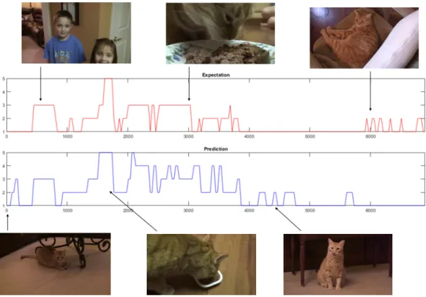
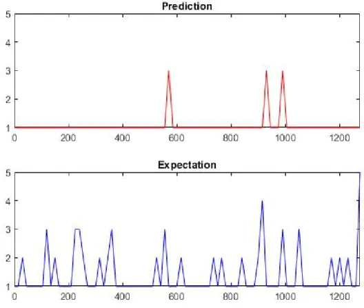
classes exist in these videos which increases the types of videos that can be processed. A sample output from the model showing how the scores are tracked throughout the video is shown in Figure 4.1. Using the sample output as an example, it can be seen what people rated as important in the example video. The events of the children appearing, and the cat eating were rated as medium to high importance. The cat sitting or laying down was found to be less important in relation to the overall video, and therefore would be excluded from a summary.

Figure 4.1: Example Output with both Expectation and Prediction scoring Shown

4.4 Training

In every network configuration, Adam [25] was chosen to be the optimizer and the batch size was always 32. Validation splits of 80-20 were always used in the testing of the networks as well. We found 20 epochs was long enough that training was

(32)

completed in that time. For the metrics, the loss function used was categorical cross entropy [26] since we were sorting into 5 unique classes.

(33)

Chapter 5

Performance Analysis

5.1 Modality Comparison & Analysis

To analyze the first experiment that was focused around three variables, we break up the results so each variable can independently be analyzed, as well as by dataset. To compare these results, the average of all runs was taken for the given category that is being analyzed. For example, when analyzing the full scale we take the runs that did not downscale and average them all together regardless of the other variables. This means the audio, video, and combined accuracy and loss scores were all averaged together, as well as the data from both interval options. The resulting averages only differ in the scaling of the data and aren’t reflective of other changes. This was done for each of the different variables, so scaling analysis compared run averages of full, half, and quarter scale, interval analysis used averages of all runs at either full or half scaling, and the modality analysis used averages for audio, video, and the combined data.

5.1.1 TVSum Analysis

5.1.1.1 Scaling

First we can examine the effect that the scaling of the data had on the results. For the scaling naming conventions, the fraction is per dimension, so the full scale size is

(34)

CHAPTER 5. PERFORMANCE ANALYSIS

224x224, the half scale is 112x112, and the quarter scale is 56x56. The accuracy and loss graphs are shown in Figure 5.1.

Figure 5.1: Scaling Accuracy and Loss Results

Based on the graphs it can be seen that during the training phase the down-scaling of the data hurt the accuracy. During the validation phase however, the results all ended at almost the exact same value. With the validation phase more closely representing the prediction of the model, it can be said based on these results that the scaling has little to no overall effect on the results. So although some data is loss with down-scaling, it is more efficient to train at the lower resolution.

5.1.1.2 Interval

Next, we can examine the Interval and its effect on the final result. For the interval result naming, the result labeled half refer to those that have an interval equal to half the video’s frame rate. So for 30 frames per second video, a full interval is a sample every 30 frames, whereas half interval is a sample every 15 frames, resulting in twice the amount of data. The accuracy and loss graphs for the interval testing are shown in Figure 5.2.

(35)

Figure 5.2: Interval Accuracy and Loss Results

Similar to the results of the interval testing, the training and validation data have differing results. Also similar to the previous results, the more data in the test, the better the training result. For the training phase, the half interval performed better than the full interval. However during the validation phase, the results again almost the same. In this case, the difference is .008, or 0.8%. Based on this, it can be said that it is most efficient to create a model using the full interval model, as there is very little loss of data, compared to doubling the size of data.

5.1.1.3 Modality

Finally, we can compare the results based on the modality of the data used. Figure 5.3 shows the resulting accuracy and loss.

Figure 5.3: Modality Accuracy and Loss Results

(36)

the combined model, followed by the audio model. During the validation phase how-ever,the video performed the worst and the audio and combined models performed equally as well, but better than the video model. Based on these results, the com-bination of the video and audio would be the best model to train. The reason that the combination model is better than the audio model is that based on the training results. With the higher training results, any data that is reflective of the training set will perform better with the combination model compared to the audio model.

5.1.1.4 Examples

Based on the three different variables tested, the preferred setup for a model is quarter scaled, full sampling interval, and the combination of both audio and video data. For the following examples, that is the model that was used to generate the predictions. First, the F-score can be calculated for the categories and the overall dataset. The table is shown in Table 5.1.

(37)

Table 5.1: F-Scores for TVSum Categories

Category Average F VT 12.51168 VU 14.68768 GA 14.02588 MS 19.90464 PK 16.32025 PR 17.16969 FM 18.31854 BK 14.32708 BT 21.40472 DS 18.18556 Total 16.72462

To calculate these scores, the F-Score was calculated for each summary of the videos. The summaries were created by taking the top 15% of scores. The categories listed are those referenced in Table 4.1, with the overall total average being listed as ’Total’. The overall range of the scores is 8.8930379.

(38)

Figure 5.4: TVSum Example 1

Figure 5.4 shows the first example prediction for the TVSum dataset. This ex-ample had the highest F-score, for the model of all the videos, at 33.83. Looking at the trends between the graphs, it can be seen that in the center where the lower score density is less, the prediction reflects this with a larger gap between important scores and a lower overall score. In other areas where low score density is higher, the prediction tends to estimate high, with scores of 5 being common in these areas.

(39)

Figure 5.5: TVSum Examples 2 & 3

Figure 5.5 shows two different predictions. The prediction on the left predicts a score of 1 for the entire video. The prediction on the right shows a prediction that although as not as clear as the example in Figure 5.4, does follow a trend of the expectation. In areas where a score of 3 or higher is detected in the expected value, there is typically a high score seen in the prediction. When we evaluate with F-score however, the prediction on the left scores 27.94. The prediction on the right scores 0. This is due to the way F-score is calculated. Since no prediction score directly matches the expectation, the result is not able to be calculated to due a division by 0, resulting in an F-score of 0. This shows that there is a need for subjective testing when it comes to video summarization.

5.1.2 SumMe Analysis

Similarly to TVSum, the models trained on the SumMe dataset can also be analyzed. The same naming conventions and methodology apply as with the TVSum dataset analysis.

5.1.2.1 Scaling

(40)

Figure 5.6: Scaling Accuracy and Loss Results

For the training phase, the results performed best to worst based on the amount of data available, the as was seen in the TVSum results. During the validation phase however, the Full scale continued to be the best be a noticeable margin. The difference was .0347 or almost 3.5% which is significant. The loss numbers however are almost all equivalent.

Based on these results, the models trained on SumMe that do not downscale are going to be the best ones to use due to the increased accuracy.

5.1.2.2 Interval

The results of the interval tests on the SumMe dataset are shown in Figure 5.7.

Figure 5.7: Interval Accuracy and Loss Results

For the interval test, the models that learned when the sampling interval was half the frame rate performed better during the training phase. Similarly to TVSum

(41)

though, during the validation phase they were almost exactly the same value. As the validation more closely reflects the actual predictions, the better model to use would be those trained when the sampling interval is equal to the frame rate, as these are more efficient.

5.1.2.3 Modality

The results of the modality comparison tests on the SumMe dataset are shown in Figure 5.8.

Figure 5.8: Modality Accuracy and Loss Results

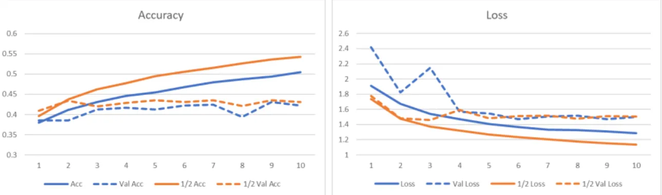
It can be seen from the results that during the training phase, the video performs the best by a small margin, with audio and the combination of both data types being equal at a slightly lower accuracy. However during the validation phase, the combined model performs slightly better than the audio, and much better than the video model. For these reasons, the combined model using both the video and audio data is the best for creating summaries.

5.1.2.4 Examples

Based on these three tests on the SumMe dataset, the best model to use would be one that does not downscale the data, samples the data at a rate equivalent to the video frame rate, and uses both the video and audio data.

(42)

Again, looking at at the F-Score for this dataset, the overall F-score came to be 19.4311111. The highest f-score for any video was 48.22. This prediction is shown in Figure 5.9.

Figure 5.9: SumMe Example 1

Looking at the first example, it can be seen that when the prediction was a score of not 0, it was an accurate reflection of the expected value. However, for a majority of the time it learned to not predict an importance. In this example, much of the video was scored as 1 for the expectation, so the model simplification is understandable.

(43)

Figure 5.10: Sume Examples 2 & 3

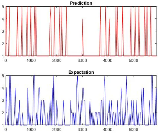
Similar to the situation in TVSum, Figure 5.10 shows two predictions where the higher F-score doesn’t seem to match the expectation. The prediction on the left scored an F-score of 38.26. The figure on the right again scored 0, similar to the previous case. When examining the graphs for ourselves, it can be seen that the prediction on the right looks much more accurate in terms of following the expectation. This is yet another example of where F-score doesn’t seem to accurately reflect how well these summaries perform.

5.2 Classification Model Analysis

For the second experiment, we want to analyze the performance of the 7 different summarization dense networks, as well as continue to analyze the general trends across the modalities.

5.2.1 TVSum

5.2.1.1 Dense Video Models

First we examine the results of the dense networks that were trained and tested using only the video data. Both the accuracy and loss results are shown in Figures 5.11 and 5.12.

(44)

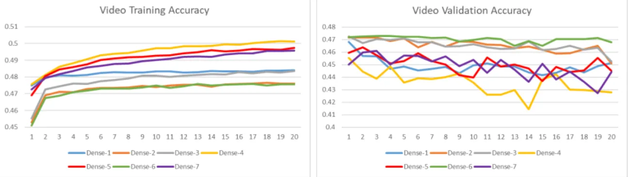
Figure 5.11: Video Accuracy Results

Figure 5.12: Video Loss Results

Among the 7 dense networks, Dense-4 performed the best during the training phase finishing at 50.1% accuracy whereas Dense-2 and Dense-6 performed the worst during training at about 47.6% training accuracy each. The notable difference be-tween these two network configurations is the use of dropout and batch normalization in Dense-2 and Dense-6. The full list of configurations can be found in Table 3.1. This trend however is inverted during the validation phase. The highest performing model is Dense-6 which reached a validation accuracy of 46.8%. The worst perform-ing model was Dense-4 which only reached 42.8% accuracy. So while dropout and batch normalization reduced performance of the training phase, the validation phase benefited from their addition. Dense-6 performed almost equivalently between the phases, where Dense-4 suffered a large drop in accuracy. This suggests that Dense-4 is over fitting to the data due to the lack of those optimizations. Comparing Dense-2 to Dense-6, the difference is that Dense-6 has 2 extra layers. While these models

(45)

performed almost identically during training, the extra layers aided the validation, with Dense-2 only validating at 45.1%.

Looking at the loss data, these trends remain generally true. In the training phase, Dense-4 has the lowest loss among the configurations, whereas Dense-2 and Dense-6 has the highest loss. In validation, Dense-4 instead has the highest loss compared to Dense-2 and Dense-6 having the lowest.

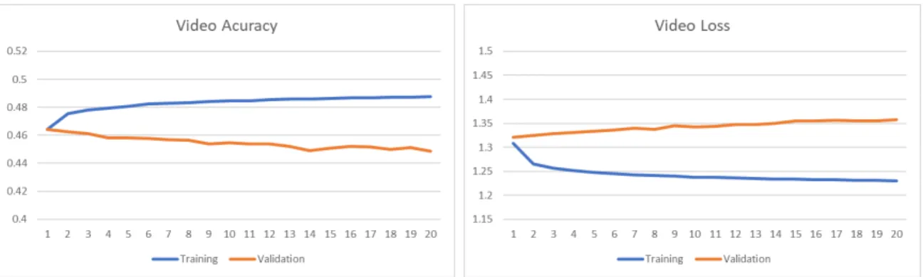
Figure 5.13: Video Average Results

Looking at the average among all 7 of the models, shown in Figure 5.13, the highest training accuracy was 48.8% whereas validation reached 46.4%. Overall, the models tended to over fit the data, resulting in the lower validation accuracy.

5.2.1.2 Audio Models

Next, the same analysis can be conducted on the models trained only using the audio data. The accuracy and loss results for these models is shown in Figures 5.14 and 5.15.

(46)

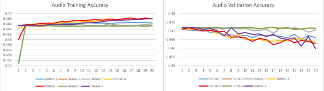
Figure 5.14: Audio Accuracy Results

Figure 5.15: Audio Loss Results

Looking at the accuracy numbers first, the results look quite different than the video results did. The audio training data numbers are much more closely grouped than the video was, with every model finishing within .003 points of each other. Dense-4, Dense-5, and Dense-7 all finished within .0016 of each other around 46.8% accuracy. Dense-2 and Dense-6 finished as the worst performing models at 46.5%. This is interesting as this matches the video training results. With the models all being so close in accuracy however, it is difficult to say that the configurations made a significant difference.

When examining the validation data however, the data has stronger trends that can be examined. Similarly to the video, the worst performing models from training performed the best, which were again Dense-2 and Dense-6. These models actually had a higher validation accuracy than training, with both models validating at 47.2% accuracy compared to 46.5% during training. This suggests that these audio models

(47)

were actually under fitting the dataset. The worst performing model was Dense-7 which fell from 46.8% during training down to 46.0% during validation.

Figure 5.16: Audio Average Results

The average results for the audio models are shown in Figure 5.16. Similarly to the video data, the models tended to over fit, however not as severely in this case. The average Audio model reached 46.7% accuracy during training while validation reached 46.4% accuracy. So while the average model performed worse during training, both the video and the audio finished the validation stage around 46.4%.

5.2.1.3 Pre-Fusion Combined Models

Finally, the combination models utilizing both video and audio can be analyzed to determine how viable the classification method is when utilizing the TVSum dataset. The accuracy and loss numbers for these models are shown in Figures 5.17 and 5.18.

(48)

Figure 5.18: Combined Loss Results

From the graphs it can be seen that one model stands out compared to the others. Dense-3 in training performed significantly better than all other models, reaching an accuracy of 62.6%. This model was unique in that it was the model that had more nodes per layer than the other models. It also utilized both dropout and batch normalization. As can be seen in the validation data however, this model heavily over fit the data, and performed significantly worse than all other models, reaching only 38.0% at the end of the validation phase. The remaining models however all performed similarly to the single modality models. Dense-4 performed the best of the remaining models during training reaching 50.4% accuracy, while the worst performing models were again Dense-2 and Dense-6 at 47.5% and 47.6% respectively. The validation data again supports the previous claims, with the worst performing models from the training being the best performing models. Dense-2 performed the best with a 46.6% accuracy rating, while Dense-4 fell to 43.8%.

(49)

Based on the averages of the combination models, shown in Figure 5.19, the combination models were the most accurate of the three sets during training. During Validation, they were the lowest of the three models. The average accuracy for the models reached 50.9% during training and 46.3% during validation. When the outlier model in Dense-3 is removed from the calculations however, the new average during training is 48.9% with validation reaching 46.6%. The numbers without Dense-3 are almost identical to those found during both the video and audio tests.

5.2.1.4 TVSum Final Analysis

When comparing the 3 sets of models, the results all supported each other. In each case, Dense-2 and Dense-6 were the least likely to over fit the data. They also suffered almost no change in accuracy when comparing the training phase to the validation stage. The final step in the analysis of these models is comparing the F1 scores. This is typically the measurement associated with video summarization as the final quantifier of its accuracy.

One item to note is the shape of the graphs throughout. The training accuracy graphs tended to follow the expected trajectory or rising sharply at first and leveling off as time continued. The training losses reflected this with a steep drop in loss at first, and smoothing as time continued. The graphs during the validation stage however did not follow these trends. During the validation stages, the graphs were notable jagged with many different points of rising and falling, and trends less obvi-ous. The average graphs reflect this with the slopes of the lines not aligning. These observations lead us to believe that the models had trouble with learning the TVSum dataset. This could be for a number of reasons. One of these is that the videos in TVSum are grouped into categories. With categories that contain many similar objects, the classifications will be based upon similar situations. For example, one category within TVSum is vehicle repair, and a second category in TVSum is Dog

(50)

Show videos. There are very few classes that overlap between these two categories. Our theory behind the summarization after classification is that the summarizer will begin to learn class relationships. With few overlapping classes between videos, there is less value in learning those videos. So when the videos are limited to categories, it is imperative that a sufficient number of classes overlap between categories. This could be a major reason that we see such large spikes and changes among the validation data. When the models begin to learn one category of videos better than another, the validation accuracy begins to reflect how that category compares to the others.

The typical metric used to measure the accuracy of a video summarization model is F-Score, rather than accuracy or loss. This is because it is better able to represent how far from the truth the summary is than accuracy is able to. Table 5.3 displays the F-Scores for each category as well as the overall F-Score for the entire dataset. Both Dense-2 and Dense-4 are displayed to compare the models that performed the best and worst in each phase of learning.

(51)

Table 5.2: F-Scores for Dense-2 and Dense-4 for TVSum

Dense-2 F1-Scores

Category Video Audio Combined VT 0.16742 0.21208 0.21864 VU 0.22346 0.22722 0.18476 GA 0.20202 0.20236 0.2243 MS 0.2224 0.24812 0.18538 PK 0.20738 0.2228 0.21016 PR 0.19776 0.23382 0.18802 FM 0.20928 0.2338 0.1732 BK 0.20642 0.2258 0.18 BT 0.23692 0.20798 0.18962 DS 0.1904 0.2305 0.18904 All 0.2089 0.2068 0.1795 Dense-4 F1-Scores

Category Video Audio Combined VT 0.079755 0.176866 0.160622 VU 0.145506 0.251812 0.084599 GA 0.112373 0.230657 0.097492 MS 0.08179 0.125552 0.080057 PK 0.110434 0.129719 0.141394 PR 0.117086 0.120964 0.142175 FM 0.165948 0.117753 0.085717 BK 0.113667 0.152308 0.056322 BT 0.226391 0.237184 0.110621 DS 0.086191 0.147375 0.105503 All 0.122383 0.164543 0.107607

When we begin to analyze the F-Score we see results that are different than those we saw from the accuracy and loss. Looking at the dataset as a whole, Dense-2 performed almost equally between Video and Audio, while the combined F-Score was much lower, suggesting that combining the data was actually not beneficial. In Dense-4, a different story is true. Audio heavily outperforms the video, with the combination resulting in an even lower accuracy. There also seems to be no real bias towards any category. The model doesn’t favor any of the categories which is actually intended. One of the goals of this approach was to make a generalized model that is not application specific. With no category significantly outperforming the others across all 3 data sources, this seems to be the case.

To get another understanding of what is actually happening, the output summaries are useful. The first example is a tutorial video of how to clean your dogs ears. This

(52)

video features a mix of text slides along with video, and music mixed with talking. For the graph, the video, audio, and combined predictions are shown along with the ground truth expected value. The x-axis is the frame number, with y representing the prediction for that frame in the video on the 1-5 importance scale, thus creating a timeline of importance as the video progresses. These examples were taken using the Dense-2 Network specifically. The first example is shown in Figure 5.20

Figure 5.20: TVSum Example Output 1

From this example we find that the video tends to take the lead with the prediction, with the audio acting almost as a filtering effect. One leading example of this is shown at the 1500 frame mark. In the video prediction there are multiple spikes in prediction from 3 down to 0, whereas the audio has a constant line at 0 importance. The combined prediction took both data inputs and the result is a flat line occurring at a level 3 importance over that section. This is the filtering effect that was mentioned. Looking at the same frame count in the expected values, the prediction has a spike from 5 down to 2, with the average looking to be around 3. This filtering effect was a common theme among examples, where the combined prediction utilized the values of the video summary more often but applied the shape of the audio summary more

(53)

often. A second example is shown in Figure 5.21.

In the second example video, a similar sampling effect can be seen specifically at the points the audio prediction spikes. Although the audio prediction is marking these as a 0 importance, that is not reflected in the combined prediction. The shape however is reflected, with those spiking values showing up in the combined prediction. One example of where this benefits the summary to match the expected values is around the 800 frame mark. The inverse effect is also shown with spikes in the video prediction that are incorrect being smoothed to lower values. One example happens near the 4500 frame mark. The F-Score for this summary was 10.53, however looking at the key spikes it is shown that the combined prediction actually is aligning fairly well. An important note is that video summarization is about capturing the most important parts of a video. This can be seen in Figure 5.22.

(54)

Figure 5.22: TVSum Example Output 2, Scores of 3 or above

When we zoom in on scores of 3 or above as shown in Figure 5.22, the similarity between the prediction and expectation becomes more evident. This continues the discussion of what the best metrics for video summarization are. We discuss the F-score metric more in section 6.2.

This filtering effect however is not only beneficial to the summary. We also found multiple examples where this effect has a negative effect on the prediction. One of these examples is shown in Figure 5.23.

(55)

As can be seen in Figure 5.23, the video prediction has many spikes, similar to the expectation. However the combined prediction has many constant sections, like the audio prediction. This is detrimental to the combined summary. Looking at the area from around frames 500-750 in the video prediction it can be seen that it almost matches the expectation. The combined summary smoothed these spikes to a constant prediction, which is worse than the video prediction. So although in some cases the combination helped as shown in the previous examples, there have also been cases where the combination has hurt the result.

Finally, we can also examine the post fusion model. To create this, the video and audio outputs were averaged, and a summary was created from those results. The data averaged in this case was from Dense-2 as that was the best scoring Pre-Fusion model.

(56)

Table 5.3: F-Scores for Dense-2 Post-Fusion on TVSum

Category F-Score VT 0.2201962 VU 0.1636618 GA 0.0949427 MS 0.1681878 PK 0.1280141 PR 0.1112792 FM 0.1898702 BK 0.0938838 BT 0.1093584 DS 0.1938902 All 0.149511185

Interestingly, the Post-Fusion model averaged similar to the best Pre-Fusion model. The overall average was slightly lower though. This is as expected as the Pre-Fusion model is specifically trained on the problem, compared to the Post-Fusion model which instead averages trained data. So although the Post-Fusion model was not better, it was still performed well compared to the other models.

5.2.2 SumMe Analysis

5.2.2.1 Video Models

The same analysis can be performed on the SumMe dataset as the TVSum dataset. The models tested were the exact same models as TVSum, with the configurations found in Table 3.1. We analyze the models trained only using the video data first. The accuracy and loss for these models is shown in Figure 5.24 and 5.25.

(57)

Figure 5.24: Video Accuracy Results

Figure 5.25: Video Loss Results

Based on the graph of the 7 models, we can see that Dense-5 performed the best during training of the models, reaching 84.6%. The worst performing model was Dense-6 at 72.7%. The data from the validation stage of learning shows a different story however. Similarly to the TVSum models, the best performing models from training perform worse during the validation stage as the data beings to over fit the dataset. Dense-5 fell from 84.6% all the way to just 55.2%. Dense-6 improved in performance, reaching 74.0% accuracy. The differences between these two models are the inclusion of dropout and 2 extra layers in Dense-6.

The average results for all of the models trained on the video data are shown in 5.26.

(58)

Figure 5.26: Video Average Results

Similarly to the TVSum video models, the average model trained better than the validation model. The average model reached 76.7% accuracy while training, while peaking at 74.0% accuracy during validation. The shapes of these graphs however differ from the TVSum models. Examining the loss graphs specifically, one notable feature is that the curves all follow a similar trajectory during both training and validation stages. This is compared to the TVSum dataset that had unstable loss graphs and less obvious trends.

5.2.2.2 Audio Models

The results from using only the audio from the SumMe Videos are shown in Figures 5.27 and 5.28.

(59)

Figure 5.28: Audio Loss Results

Once it can be seen that the models followed the trend of previous experiments. During the training phase, Dense-5 performed the best of all the models at 74.8% accuracy. The worst performing model was Dense-2 at 72.6% accuracy. During the validation stage, Dense-5 fell to 69.6% accuracy and was the worst performing models, whereas Dense-2 improved to 74.0%. These results are consistent with the previous video model findings.

The averages for the audio models are shown in 5.29.

Figure 5.29: Audio Average Results

From the figure it can be seen that the average audio model reached 73.3% ac-curacy during training while peaking at 74.0% during validation. Like the video models,the general curve shape is more aligned to the expectation compared to the TVSum audio models. This is best seen in the validation loss graph where the shape resembles the training data. The validation accuracy graph doesn’t closely track the

(60)

training curve, however the results are much more stable and consistent compared to those seen in the TVSum results.

5.2.2.3 Pre-Fusion Combined Models

Finally, the results of using both the video and audio data from the SumMe dataset to train combined models is shown in Figures 5.30 and 5.31.

Figure 5.30: Combined Accuracy Results

Figure 5.31: Combined Loss Results

From the figures we see that the previous trends continue to be present themselves in the combined model. Dense-5 is again the best performing model during training reaching 86.7%. Dense-6 was the worst performing model at 73.6% in this case. The validation data again is a reversal of the training data, with Dense-6 having the highest accuracy at 74.0% and Dense-5 being the second lowest at 61.3%. The lowest in this case was Dense-1 at 60.1%.

(61)

The averages for the combined models are shown in Figure 5.32.

Figure 5.32: Combined Average Results

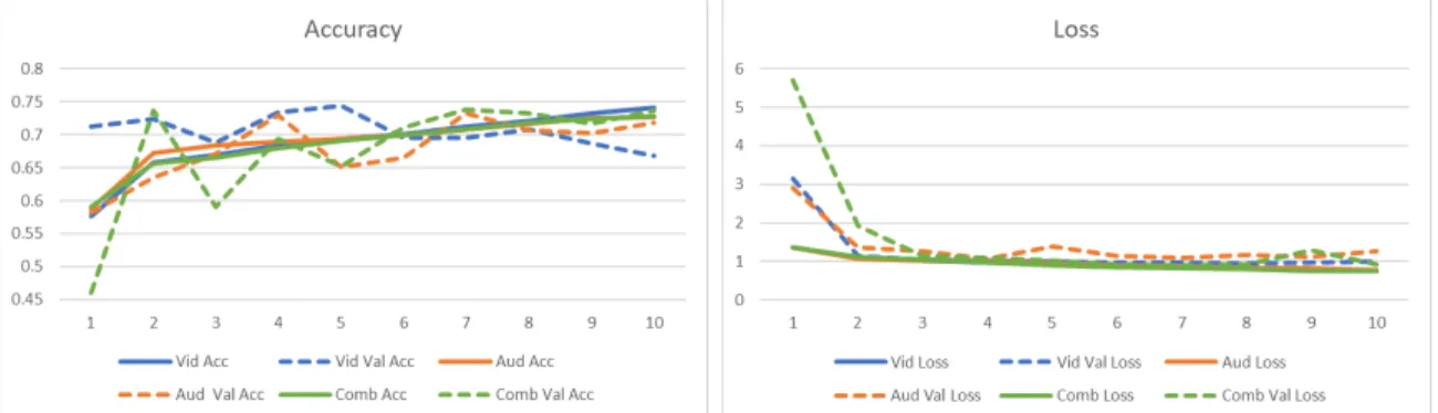
For the combined model average scores, the results are close to those of both the video and audio which is as expected. The combined accuracy reached a peak of 77.8% while training which is higher than the audio or video when they are separate from each other. While validating, the final result is 74.0% which matches the separate validation models.

5.2.2.4 SumMe Final Analysis

Overall, the SumMe models performed better than the TVSum Models. All three sets of models were consistent and similar to each other, with the expected results of the combined model being slightly better while validating and the audio model being slightly worse. In all three cases, Dense-5 outperformed during the training stages while under performing during the validation stages. Dense-2 and Dense-6 were consistent between training and validation in each case, where although performing the worst in the training phase, would perform the same or better during validation resulting in them being the best performing models of the group. These results align with what was previously seen in TVSum.

When comparing TVSum vs SumMe, there are two key points to note. The first is that the SumMe models performed better in terms of overall accuracy compared to TVSum. This conflicts with what the state-of-the-art models say as well as previous

(62)

video summarization models. The second important note that helps to explain this has to do with the shape of the graphs. It can be seen that the TVSum graphs had many spikes, with large changes occurring. The resulting graphs did not follow what we would expect typical training graphs to look like. The SumMe graphs however, do more closely align to these expectations. We believe this is due mainly to the dataset structures. TVSum is comprised of separate categories, compared to SumMe which has different types of videos that aren’t categorized. With the classification approach that is being taken, we believe that the overlap of classes observed in a video directly correlates to effectiveness. When videos are categorized such as in TVSum, there are many examples of classes that are being learned, but all within similar environ-ments. For example, in a car repair video a tire will often be seen alongside a wrench. With multiple car repair videos, this association of tire and wrench becomes stronger. When a wrench is seen on its own though, the summarizer struggles as the class re-lationships between what is being observed don’t exist. If instead there are examples of a wrench alongside a tire, a stove, and plumbing, the summarizer begins to form relationships of importance based upon multiple different class dependencies. This is why the uncategorized videos of SumMe may be performing better during learning. By removing the restrictions of video type, you begin to remove the restrictions of the environments that the classes within the videos are being learned in.

Moving to the F-Score performance metric, we can again look at the totals by modality and model, as well as look at examples to compare results. The results are shown in Table 5.4. Like the TVSum analysis, the models that performed at the two different ends of the spectrum while learning are shown, being Model 2 which performed best while validating and Model 5 which performed best during training.

(63)

Table 5.4: F-Scores for Dense-2 and Dense-5 for SumMe

Dense-2

Video Audio Combined 5.187 12.06 1.66

Dense-5

Video Audio Combined 4.26 7.37 14.43

Unlike TVSum, Dense-2 worked best when both audio and video were used to-gether. The best performing training model, Dense-5 in this case also had a similar trend where the video was the worst performing, audio was the best performing, and the combined was in between the two. Another important note is that although the numbers for loss and accuracy between the SumMe and the TVSum models were quite different, the F-scores are similar.

Looking now at the examples, we can see trends begin to appear similarly to the TVSum models. For the SumMe models however, the trends aren’t as clear. Each model seemed to have fixated around different points. This is shown in the first example, seen in Figure 5.33.

Figure 5.33: SumMe Example Output 1

(64)

model seems to do the opposite, favoring a score of 0 and spikes up to 4. The combined model reflects this by outputting a majority of scores at a level 3 importance. This happened across many of the videos, with the video scores favoring a higher scoring while the audio favoring low scores. Often times this results in the combined model returning many scores around a 3. Another example of this is shown in Figure 5.34.

Figure 5.34: SumMe Example Output 2

In this case, the video model again centered around a score of 4 with the audio centering around a score of 2. Similarly to TVSum, a filtering effect can start to be seen, but in reverse this time. In this example, the audio shape is more closely followed, with the weighting being pulled up by the video scores.

Another example of the audio and video working well together is shown in Figure 5.35.