Excited States and Transition Metal Compounds with Quantum Monte Carlo

(1)

Excited States and Transition Metal Compounds

with Quantum Monte Carlo

Von der Fakultät für Mathematik, Informatik und Naturwissenschaften der Rheinisch-Westfälischen Technischen Hochschule Aachen zur Erlangung des akademischen Grades einer Doktorin der Naturwissenschaften genehmigte

Dissertation vorgelegt von Diplom-Chemikerin Annika Bande aus Duisburg

Berichter: Universitätsprofessor: Dr.rer.nat. Arne Lüchow Universitätsprofessor: Dr.rer.nat. Wolfgang Stahl

Tag der m¨undlichen Pr¨ufung: 14. Dezember 2007

(2)

This work is dedicated to Tante Ille

Ilse Marie Neilson (12/31/1914-02/01/2004), gentely called Tante Ille, was my nanny. She always dreamed of joining me, when I get the academic degree of a doctor of science. I have to thank her a lot for what she taught me: to meet life with humor and confidence.

(3)

Before all others I owe Prof. Dr. Arne L¨uchow a dept of gratitude. His nonstop support made a success of the time in his group. I am especially thankful for having had many opportunities to take my time for personal studies and to attend inspiring conferences.

I thank Prof. Dr. Wolfgang Stahl as the second referee of this thesis.

I am thankful to Prof. Dr. Andreas G¨orling and Dr. Fabio Della Sala for their collaboration in the work on the Rydberg excitations. I further want to acknowledge the “Gesellschaft Deuscher Chemiker” (GdCh) for providing a fellowship to travel to the 1st _{European Chemistry Congress. Though not by names I wish to mention all the} organizers of conferences and seminars who offered me the opportunity to present my work. Furthermore I want to thank the reseachers I became acquainted with.

Many thanks to Hanno Heeskens who guaranteed a smooth course for all computa-tional concerns as well as to the people from the “Rechenzentrum” of RWTH Aachen University.

The correction of this thesis has been done by Martina Peters, Clemens Minnich, and Raphael Berner, to whom I am grateful.

I am very thankful to have had Anja Simon as a colleague and roommate from the beginning of my Ph.D. studies. She has always been and is still interested in my work and, which is most important, has become a very close friend of mine.

Furthermore I wish to express my thanks to my other three roommates Jan Sielk, Sandra K¨uttner, and Thomas Wieland to the other two quantum Monte Carlo grad-uate students Raphael Berner and Annett Schwarz, as well as to Michaela Braun for fruitful discussions and good collaborations. I offer my thanks to the research students Michael Wessel, Jens Burghaus, and Jaswinder Singh who worked on the vanadium oxide compounds. I am grateful to Iwona Mennicken for her help on all non-scientific questions. My gratitude shall be expressed to the colleagues from the “Institut f¨ur Physikalische Chemie” for a good working climate.

I very much appreciate my close friends, my family and my husband for their never ending emotional support.

(4)

To the most challenging electron structure calculations belong weak interactions, excited state calculations, transition metals and properties. In this work the performance of variational quantum Monte Carlo (VMC) and fixed-node diffusion quantum Monte Carlo (FN-DMC) is tested for challenging electron structure problems using the quantum Monte Carlo amolqc code by L¨uchowet al..

The transition metal compounds under consideration are vanadium oxides. Here excita-tion, ionizaexcita-tion, oxygen atom and molecule abstracexcita-tion, and atomization energies have been studied for the vanadium oxide clusters VO+n/0withn= 0−4. The reaction energy of V2O5 → VO3+VO2 was calculated. The complete FN-DMC procedure established includes geometry optimization and calculation of zero point corrections using BP86/TZVP, single point cal-culation of the BP86/SB type, and optimization of Jastrow parameters in the framework of VMC variance minimization to obtain a suitable guide wave function. A careful adjustment of the pseudopotential evaluation and of the time steps was done to obtain reliable FN-DMC results that proved at least as accurate as results from CCSD(T)/cc-pVTZ calculations in-cluding scalar relativistic corrections. This FN-DMC procedure will easily be extendible to larger systems. For the oxygen abstraction and the atomization where experimental data is available for comparison, FN-DMC/BP86/SB always renders the best results of all calcula-tions performed. The dissociation of VO, its vertical ionization and the oxygen abstraction from VO+₂ are obtained in excellent agreement to experiment using FN-DMC/BP86/SB.

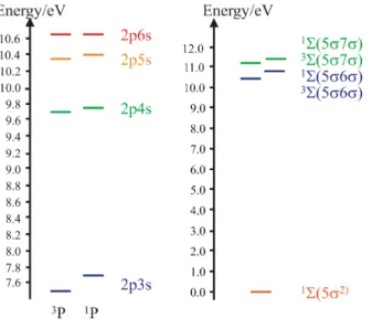
Rydberg excitation energies and singlet triplet splittings are calculated for the carbon atom and carbon monoxide. The considered excitations were from the3P ground state into the 3P and 1P 2pns (n=3-6) Rydberg states and from 1Σ into 1Σ and 3Σ 5σmσ (m=6-7), respectively. The wave functions used are described in terms of configuration state functions from OSLHF orbitals which are particularly well-suited for the construction of QMC guide and trial functions for Rydberg states. The OSLHF excitation energies are improved with VMC and FN-DMC, respectively. However, fixed-node DMC does not describe the singlet triplet splittings reliably whereas VMC results are in excellent agreement with the experi-ment. Regional analyses and the newly established weighted FN-DMC approach were able to improve also the DMC singlet triplet splittings over OSLHF and the novel technique can be equally used for the treatment of other excited state systems.

(8)

Chapter 1

Introduction

Quantum Monte Carlo methods are capable of solving the full three dimensional electronic Schr¨odinger equation numerically even for large molecules. Stabilization, reaction or excita-tion energies among other properties can be calculated from first principles. Two basically different quantum Monte Carlo (QMC) methods are most commonly used and widely applied in electron structure theory: variational and fixed-node diffusion quantum Monte Carlo.1–8

In variational quantum Monte Carlo (VMC) the expectation values for the Rayleigh-Ritz quotient is evaluated using the stochastic Monte Carlo integration and a many-electron trial wave function. It contains a linear combination of Slater determinants generated in ab initio

calculations and the so-called Jastrow function. The latter explicitly accounts for dynamic electron correlation and can be adjusted by minimizing the VMC energy or variance.9,10

In the diffusion quantum Monte Carlo (DMC) procedure,11_{the imaginary time equivalent} of the electron motion is simulated according to a stochastic diffusion process evolving to a solution of the imaginary time Schr¨odinger equation. A fermionic system is calculated by propagation of the wave function in time starting with a guide function of the same type than the VMC trial function. In the fixed-node extension of the DMC method (FN-DMC), the guide wave function’s nodal hypersurface determines the accuracy in acting as additional boundary condition.12 Its nodes need to be exact to sample the exact energy. This is an actual research topic, because it is not known how to routinely improve these nodes.

The first works on QMC go back to the 1960ies though the most essential steps in its history were made 10 years later. At that time Hartree-Fock and post Hartree-Fock theories as well as density functional theory were already much further developed in the field of

(9)

electron structure calculations. Only few researchers were willing to direct their attention from integral based ans¨atze to solve the Schr¨odinger equation according to a random process. However, this discrepancy was not as pronounced as the never ending argument about density functional based methods beingab initioor semi-empirical, because many more scientists use density functional theory than quantum Monte Carlo.

At the moment the quantum Monte Carlo community is relatively small, about 50 re-search groups worldwide and only four of them in Germany. No commercial quantum Monte Carlo code is available as there are several “traditional” electron structure programs. Two codes are more widespread: the Casino from the Needs group13 and the new Zori code.14 But since most research in quantum Monte Carlo aims in the development of the method and not in applied computations, most groups use private codes, as we at RWTH Aachen Uni-versity haveamolqc(Atomic and Molecular Quantum Monte Carlo Calculations) by L¨uchow

et al.15–17 Much work goes into the update of private codes and all have to prove their applicability to recent quantum chemical problems, which is were this work aims in.

To the most challenging electron structure calculations belong weak interactions, excited state calculations, transition metals and properties. Electronic structure quantum Monte Carlo methods are versatile and applicable to atoms and molecules of single-reference or multi-reference character, strong and weak interactions, as well as ground and excited states and therefore at the forefront of electron structure research.

Special emphasize on the applications of our code lies in performing cheap calculations that are extendable to large molecular systems. The way to extendability has already been paved by the favorable scaling of quantum Monte Carlo18and its good parallelizability, which allowed to set up the QMC@home project basing on the amolqcprogramm.19 Cheap in this context shall indicate the use of single-reference and one-determinant ans¨atze for the guide and trial wave function as far as possible.

This approach has already proven successful for the calculation of weak interactions in (CH4)2, (NH3)2, (H2O)2, and (C6H6)2 and for the dimerization of Antracene.20–22

Transition metal systems were studied in calculations on Cr, Fe, and Ni carbonyl com-plexes. The CO abstraction has been described accurately in most cases which does not only proof the applicability of amolqc to transition metal systems, but especially the accurate description of electron correlation which is different for reactants and products.20,21

(10)

prob-lems is continued. Inorganic transition metal compounds and excited states are studied.

The transition metal compounds under consideration are vanadium oxide clusters. Solid vanadium oxides find application as heterogeneous oxidation catalysts in major industrial processes of which the best known is the oxidation of sulfur dioxide yielding sulfur trioxide. Then SO3 is converted into sulfuric acid, the industrial chemical with the largest production volume. A very innovative approach for the functionalization of methane is the direct partial oxidation to methanol and in a prior step the activation of C-H bonds.23 In connection to that the aggregation of CH4 on different V2O5 surface clusters has been studies using density functional theory methods.24,25 They are planned to be performed with FN-DMC which offers an accurate description of electron correlation and therefore of dissociation energies. The most essential catalytic step is the oxygen abstraction and uptake which is studied for all vanadium oxide clusters presented in this work. Furthermore, the atomization energies and several reaction energies are studied to test the general performance of the method. Excited states of the transition metal atom are approached and as another topic, for which the description of electron correlation is challenging, the ionization of VOn(n=0-4) is studied. Special emphasis lies in the testing and discussion of single-determinant guide functions and pseudopotentials.

The challenge of treating excited states was posed by the calculation of low lying Rydberg states of the carbon atom and carbon monoxide.26,27 The accurate calculation of excitation energies usually requires a method that accounts for the correlation energy which is generally smaller in the excited than in the ground state. DMC is known to be a versatile method for this purpose. However, calculations turned out to be difficult in all cases in which the wave function displays a complicated nodal structure or suffers from spurious nodes due to basis set deficiencies.28,29 Therefore, as climax of this study, the weighted FN-DMC approach for excited states has been developed.30

(11)

Chapter 2

Electron Structure Calculations

Chemistry is the science of transformations and aggregations of matter. For a profound understanding of the concept of chemical bonding, reactions, and molecular properties it is necessary to have a picture in the atomic scale in mind. Here, the behavior of electrons takes over the fundamental role. Electron structure theory is the field of theoretical chemistry in which these electronic concepts are studied by means of quantum mechanics, chemistry, physics, mathematics, and computer science. The central equation is the Schr¨odinger equa-tion

ˆ

HΨ = EΨ.

In quantum mechanics it is computationally unfeasible to describe fermionic systems larger than H+₂ exactly. The Schr¨odinger equation turns out to be unsolvable and the cal-culations become approximate. Depending on the nature of the approximations, electron structure theory displays various approaches and can be compared to a tree with three main branches:31

• orbital based,

• density functional, and

• quantum Monte Carlo methods.

The two former, which are the traditional branches, grew naturally from the differential equations evolved directly from the Schr¨odinger equation.

Orbital based approaches are well-founded as far as the chosen method fits the problem. Some questions can be solved with little effort using the straightforward Hartree-Fock (HF)

(12)

method. But some very time consuming methods exist as e.g. configuration interaction (CI), coupled cluster (CC) or multi-configuration self consistent field (MCSCF) that tie the branch heavily to earth though being able to let it grow towards the sun alias the right solution.

The second branch mentioned is wildly growing density functional theory (DFT). To a certain extent it is set up rather similar to the HF approach, but using the electrons’ density rather than their coordinates. Sometimes DFT calculations evolve themselves elegantly to the most accurate results, but sometimes they fail disastrously. From the point of view of systematic theoretical concepts, the branch grows partly to a wrong direction.

The freshest branch, cultivated by grafting, is quantum Monte Carlo. It has different roots, namely stochastics and numerical simulation. The key to solving the Schr¨odinger equation is to simulate it for sets of random variables, and with that being able to obtain the exact solution within certain error bars. The Monte Carlo branch is unfortunately only slowly growing in the shadow of the two well established ones. Fertilized by larger amounts of computer power the development of the first strong twigs is supported nowadays.

In the following the three big fields in electron structure theory will be described in detail weighted by their importance in general and especially for this work.

2.1 Orbital Based Methods

In orbital based methods the solution to an electronic structure problem is postulated to be a wave function. Without any approximation it would exactly describe the electronic state of a given system. However, approximations have to be made to keep the question tractable. The Hartree-Fock theory is the most basic approximation to describe the electronic structure quantum mechanically with a relatively simple wave function. Configuration interaction and coupled cluster raise the quality of the wave function, perturbation theory allows deviations from the ideal system by small perturbations and multi-reference approaches account for the fact that the given system occupies several states with a certain probability. Detailed discussion of the concepts of orbital based quantum chemistry and references are to be found in textbooks on theoretical chemistry.32–36

(13)

2.1.1 Hartree-Fock Theory

The explanation of the Hartree-Fock theory is basically the explanation of the concepts of quantum chemistry and its most elementary analytical solution. As mentioned beforehand the central problem inab initioquantum chemistry is to attain a solution to the time independent Schr¨odinger equation:

ˆ

HΨ = EΨ. (2.1)

Concerning a real chemical system containingM nuclei andN electrons the question explodes to be an intractable 3(M+N) dimensional problem.

The full Hamiltonian in atomic units for such a system reads:

ˆ H =− N X i=1 1 2∇ 2 i | {z } A + N X i=1 N X j<i 1 rij | {z } B − N X i=1 M X A=1 ZA riA | {z } C + M X B=1 M X A<B ZAZB rAB | {z } D − M X A=1 1 2mA ∇2_A | {z } E . (2.2)

The single terms represent the operators of the following energy contributions:

A: the kinetic energy of the electrons, with~= ₂h_π and the Planck’s constant h, the mass of

an electronme and the “Nabla squared” operator

∇2 = ∂ 2 ∂x2 + ∂2 ∂y2 + ∂2 ∂z2, (2.3)

B: the potential energy of interacting electrons (i and j) displaying by definition a positive sign for repulsion,rij is the distance between them,

C: the electron nucleus attraction (negative). ZArepresents the nuclear charge of nucleus A and riA the distance between electron and nucleus,

D: the potential describing the repulsion between two nuclei Aand B,

E: the nuclear kinetic energy;mA is the nuclear weight.

The most important simplification, not only made in ab initio methods, is to treat only the electrons explicitly. In the clamped nuclei approximation the nuclei are considered as particles of much higher mass then the electrons and therefore being fixed in their spatial coordinates. In this framework the Born-Oppenheimer approximation allows the separation of the wave

(14)

function into an electronic and a nuclear function. The electronic wave function depends on fixed nuclear and variable electronic coordinates. With that the electronic Hamiltonian changes and includes only the terms A to C of equation (2.2) and a constant instead of D. A and C can further be added to form a one particle operator

ˆ hi=− 1 2∇ 2 i − M X A=1 ZA riA , (2.4)

whereas B represents the two particle operator

ˆ

gij = 1

rij

. (2.5)

Electronic operators, wave functions, and the energy expectation value depend on nothing more than the electron coordinates

ˆ HelΨ(el) = ( N X i=1 ˆ hi+ N X i=1 N X j<i ˆ gij) Ψ(el) = EelΨ(el). (2.6) For simplicity the indexel will be neglected in the following.

A suitable wave function for a closed shell system is the Slater determinant:

Ψ(SD)= r 1 N! ϕi(r1, σ1) ϕj(r1, σ1) · · · ϕN(r1, σ1) ϕi(r2, σ2) ϕj(r2, σ2) · · · ϕN(r2, σ2) .. . ... . .. ... ϕi(rN, σN) ϕj(rN, σN) · · · ϕN(rN, σN) (2.7)

In its columns it contains the different occupied spin orbital functions ϕi(r1, σ1) through

ϕi(rN, σN) each for the same electron and in its rows the same spin orbitals ϕ1(ri, σi) to

ϕN(ri, σi) for different electrons, vice versa. Spin orbital functions are one electron func-tions. They can be expressed as the product of an orbital and a spin function: ϕj(ri, σi) =

ψj(ri)θj(σi). The spin variables σi in fermionic systems are restricted to two distinct values

±1/2. According to that the spin functions are often referred toα =θ(+₂1) and β =θ(−1₂). The molecular orbital functions (MOs)ψi are linear combinations ofν catalogued basis func-tionsχ:

ψi = X

ν

ciνχν. (2.8)

With the determinant representation of the wave function the Pauli principle in terms of the antisymmetry principle for an odd number of electron transpositions is automatically fulfilled.32 The interchange of two rows, i.e. the coordinates of two electrons, changes the sign of the determinant and thus the wave function:

(15)

Many times another representation of the Slater determinant is helpful in which it is defined as the sum of all N! two particle permutations:

Ψ(SD) = r 1 N! N! X p=1 (−1)tp_Pˆ_p[_ϕ_i(_r 1, σ1). . . ϕN(rN, σN)]. (2.10) The permutation operator ˆPpgenerates all possible permutations of electrons. The whole con-struction ˆA=PN!

p=1(−1)tpPˆp is the antisymmetrizing operator. It antisymmetrizes because

tp=   

+1 for an even number of transpositions

−1 for an odd number of transpositions.

(2.11)

To approximate the time independent electronic Schr¨odinger equation within the presented framework one has a very powerfulab initio ansatz at hand: the variational approach. Intro-ducing the Slater determinant into equation (2.6), the expectation value of the energy of the non-normalized Slater determinant wave function can be calculated from the Rayleigh-Ritz quotient: ESD= R Ψ(SD)_Hˆ_Ψ(SD)_dτ R Ψ(SD)_Ψ(SD)_dτ ≥Eexact. (2.12) In Dirac notation it reads:

ESD=

hΨ(SD)_|_Hˆ_|_Ψ(SD)_i

hΨ(SD)_|_Ψ(SD)_i . (2.13) In the usual case of a normalized wave function in terms of a Slater determinant and with respect to the one and two particle operators, solving equation (2.12) reduces to solving four and eight dimensional integrals of the form:

hϕi(r1, σ1)|ˆh1|ϕi(r1, σ1)i = [i|h|i] (2.14)

hϕi(r1, σ1)ϕj(r2, σ2)|gˆ12|ϕi(r1, σ1)ϕj(r2, σ2)i = [ij|ij] (2.15)

hϕi(r1, σ1)ϕj(r2, σ2)|gˆ12|ϕj(r1, σ1)ϕi(r2, σ2)i = [ij|ji]. (2.16) With respect to all identical integrals the following expression remains for the Ritz energy:

To solve this expression a one electron procedure is applied. This can be understood as the movement of one electron in the field generated by the others. The method is based on the canonical Hartree-Fock equations including the canonical MOsϕ0_i

ˆ

(16)

containing the orbital energiesεi and the Fock operator ˆFi defined in atomic units:1,33,34 ˆ Fi = ˆhi+ N X j=1 (2 ˆJj−Kˆj). (2.19) The so-called Coulomb operator is defined according to the Coulomb interaction

ˆ

Jiϕj(r2) =hϕi(r1)| 1

r12

|ϕi(r1)i|ϕj(r2)i, (2.20) and the exchange operator as

ˆ

Kiϕj(r2) =hϕi(r1)| 1

r12

|ϕj(r1)i|ϕi(r2)i. (2.21) These integro-differential equations (2.18) are only solvable in a iterative manner, which is the self consistent field approach (SCF). Therefore the wave function is varied in the coefficients

ciν of equation (2.8) under the restriction of orthonormal orbitals until the total energy is minimal.

In the case of a non-orthogonal wave function the task is solving a general matrix eigenvalue problem. According to Roothaan and Hall the HF equations can be represented using a separate matrixCof coefficients ciν:37,38

FC=SCε. (2.22)

Fis the Fock matrix with the Fock matrix elements:

Fst ≡ hχs|Fˆi|χti. (2.23) S is the basis function overlap matrix with the elements

Sst ≡ hχs|χti (2.24) and εis the diagonal matrix of the molecular orbital energiesεi.

The same formalism can be applied to wave functions represented as defined linear combinations of Slater determinants. This is for example the case for open shell singlet states, which require a configuration state function of at least two determinants for a proper description of spin. Further examples will appear in the following sections.

The Hartree-Fock method is feasible of rendering accurate total energies with errors of about 0.5%. At first glance these small inaccuracies seem to be acceptable, but when calculat-ing energy differences as e.g. excitation or reaction energies, both, the energy difference and the error easily approach the same order of magnitude, demonstrating that some important energy contributions are not treated at all in Hartree-Fock.

(17)

The deficiency is basically the electron correlation, a physical effect not adequately treated in the Hartree-Fock theory. In response to the insufficient treatment of electron correlation the Hartree-Fock energy deviates from the exact energy. This energetic deviation is called the electron correlation energy according to the definition of L¨owdin:39

Ecorr =Eexact−EHF. (2.25) This definition holds for RHF/ROHF (restricted (open-shell) Hartree-Fock) where each or-bital can be doubly occupied with an up and down spin electron. By contrast unrestricted HF (UHF) does include static electron correlation to a certain extent relative to the R(O)HF determinant.33

Electron correlation, which is a pure quantum effect, can be best perceived from two viewpoints: static and dynamic correlation. For real molecules of considerable size both are hardly describable within the standard methods, but depending on the system calculated, satisfactory results can be obtained, choosing an appropriate method.

Dynamic correlation accounts for the correlated motion of particles approaching one another. Concerning electrons of the same spin one speaks of Fermi correlation in this context and defines an area of reduced probability around one electron for finding a second electron with the same spin. A description of this non-classical effect is guaranteed by the anti-symmetry of the SD. The analogue electrostatic phenomenon is called Coulomb correlation. They determine the correlation between all particles included, i.e. electrons of both spins and nuclei. For a description of Coulomb correlation the wave function must contain the proper electron electron and electron nucleus cusps not all present in the HF determinant. In quantum Monte Carlo for example, it is included by multiplying the Slater determinant(s) by a symmetric Jastrow (cusp) function. DFT methods have correlation functionals focussed on the problem. Perturbation theory, configuration interaction, and coupled cluster account for dynamic correlation by including several excited state Slater determinants in the wave functions.

Static correlation is not of dominant importance for many chemical systems, but namely in those, where different states of similar energy and same symmetry to the state of interest exist. An example are compounds that include electron rich transition elements. To describe one state properly its wave function needs to have an admixture of Slater determinants for several states of similar energy to the determinant representing the leading configuration. Those approaches are therefore referred to as multi-configuration (MC) methods.

(18)

For the more advanced methods presented below, the percentage of correlation energy can be declared: Ecorr = EHF −Emethod EHF −Eexact ·100%. (2.26)

The smallest valueEexact is (often) the exact non-relativistic energy andEmethodis the total energy from the correlation approach chosen.

2.1.2 Configuration Interaction

A configuration interaction calculation make use of basically the same variational formalism as the Hartree-Fock method with the important restriction of keeping the wave function normalized. The difference is the structure of the wave function, which consists of the HF determinant Ψ(HF) = Φ0 and, in addition to that, several excited determinants. In these S refers to all single, D to double, T to triple excitations and so on.

Ψ(CI) = d0Φ0+ X i,a da_iΦa_i + X i<j,a<b dab_ijΦab_ij X i<j<k,a<b<c

dabc_ijkΦabc_ijk+· · ·

= d0Φ0+ ΦS+ ΦD+ ΦT +· · · . (2.27)

The construction of the CI wave function is based on HF orbitals. Compared to the SCF calculation done in HF, the optimization is not performed for the expansion coefficients ciν (eq. (2.8)) but for the CI expansion coefficients d.

For chemical applications Ψ(CI) _{is usually truncated at a certain level of expansion. A} CI singles (CIS) expansion including the HF determinant and all singles, means no gain over HF, since the two components do not couple. According to Brillouin’s theorem their matrix elements are zero:40

hΦ0|Hˆ|ΦSi= 0. (2.28) CI Doubles (CID) is the smallest reasonable expansion, because the most important con-tributions to Φ0 stem from pair correlation, i.e. coupled excitation of two electrons. Few more effort is CISD with the singly and doubly excited determinants having non-zero matrix elements. Furthermore the singles account for the orbital “relaxation”, when a certain multi-reference character is accomplished in the system. Then, the HF orbitals are not the optimal any more. For chemically significant systems CISD is often the largest expansion tractable. For smaller systems CISDT or even CISDTQ can be applied accounting for the double exci-tation of the “multi-reference” singles part and, which is very important (see section 2.1.4), the products of double excitations. For very small systems it is possible to carry out non-truncated CI calculations and work at the full CI (FCI) level giving the best non-relativistic

(19)

ab initio energy to be calculated for a given basis. The lack of size-consistency in truncated CI and the inaccuracy of the HF determinant is overcome, since the whole Fock space is covered. A FCI calculation with a complete basis set would exactly solve the Schr¨odinger equation.

A positive side effect for diffusion quantum Monte Carlo (DMC) is that with the exten-sion of the wave function its nodes can also be improved.

2.1.3 Multi-Configuration Self Consistent Field Methods

One important drawback of the generally applied truncated correlation interaction methods is that one is left with the Hartree-Fock orbitals as starting point for the optimization of the coefficients d. But the HF method is for example known to provide unphysical virtual orbitals. This is in cases where single excitations, that do not contribute to the energy, have a rather large contribution in the CI wave function. And this observation can be frequently made e.g. in standard organic reactions. So it is evident, that a simultaneous optimization of the CI coefficientsdand the orbital coefficientscfor each determinant included should be a further improvement.

It can be imagined that this optimization is then much more complex than either per-forming just Hartree-Fock or correlation interaction calculations. Thus fewer configurations than in CI can usually be included. The active space for the SCF iteration is defined accord-ing to the determinants that shall be incorporated and accordaccord-ing to the number of excita-tions allowed. For the former one distinguishes between complete and restricted active space (CASSCF and RASSCF). The major difficulty in MCSCF is to define a reasonable space, because all orbitals excluded do not contribute to electron correlation, making the calculation rather unbiased.

In CASSCF,41molecular orbitals are partitioned into active and inactive spaces, of which the latter is neglected. As shown in figure 2.1 a certain number of the highest occupied and the lowest unoccupied orbitals are included in the active space. [n,m]-CASSCF or CASSCF(n,m) mean that n electrons are distributed over m orbitals without any further condition, allowing single to n-fold excitations.

In the restricted active space SCF the CAS is subdivided into MOs that are doubly occupied or empty in the HF determinant (RAS1 and RAS3) and those that can either be occupied or empty (RAS2). In the former two spaces excitations up to doubles are the only

(20)

Figure 2.1: Visualization of the complete (left) and the restricted active space (right) in CASSCF.

ones allowed, whereas in RAS2 the complete spectrum of excitations is allowed as in CAS.

Besides the ability of MCSCF to describe static electron correlation accurately, it dis-plays further appealing features. One of those is the possibility to conduct state average (SA)-MCSCF calculations, in which the coefficients c and d are optimized towards a mean energy of several states. This becomes important e.g. for conical intersections or avoided crossings of a ground and its excited states or for the description of all degenerate multiplet states of an atom. Another gain is that the MCSCF wave function is much more flexible and qualitatively correct. This is an aspect interesting to diffusion quantum Monte Carlo where a function with an accurate nodal structure has to be applied.

2.1.4 Coupled Cluster Methods

The coupled cluster (CC) method for molecules is, similar to the CI theory, based on the Hartree-Fock wave function as reference ground state wave function and includes certain single, double etc. excitations by means of further Slater determinants. The functional approach is more elegant than CI with the effect of making the method size-consistent.

The coupled cluster wave function is given as:42–45

(21)

ˆ

T is the cluster operator

ˆ

T =X µ

tµˆτµ, (2.30)

with the excitation operator ˆτµ for different multiple excitations defined over creation and annihilation operators in the framework of second quantization. tµis the so-called amplitude, representing a measure of the importance of the excitation under consideration. They are basically the same as the CI coefficientsd.

With a Taylor series of exponential functions one can rewrite the exponential of the cluster operator:46 eTˆ =Y µ etµτˆµ₌Y µ (1 +tµτˆµ). (2.31)

What seems to be the truncation after the linear term is the exact series expansion, because all ˆτ_µn = 0 with n ≥ 2. This can easily be rationalized following the rules from second quantization for carrying out of twice an arbitrary single excitation ˆτ_µ2 = (ˆτ_ia)2 = ˆτ_iaˆτ_ia

from the occupied orbital i to the virtual a: The occupied orbital can theoretically only be unoccupied once and the virtual can only take one electron. Thus the quadratic and higher order excitations cannot occur and give a zero contribution.

As in CI theory it is possible to perform CCS, CCD, CCSD, CCSDT, CCSDTQ etc. calculations, that are represented by eTˆ with ˆT being ˆT1, ˆT2, ˆT1 + ˆT2+. . .. According to equation (2.31) one can see the difference to CI for example for the singles wave function including the excitationsν and ξ in a two niveau system:

|Ψ(CCS)i = (1 +tντˆν+tξτˆξ+tνtξτˆντˆξ)|Ψ(HF)i

= (1 +tντˆν+tξτˆξ)|Ψ(HF)i+ (tνtξτˆντˆξ)|Ψ(HF)i

= |Ψ(CIS)i+ (tνtξτˆντˆξ)|Ψ(HF)i. (2.32) The product term not included in the CIS wave function is referred to a disconnected quadru-ple and guarantees size-consistency of couquadru-pled cluster. Therefore for the order of excitation, e.g. CCSD is equivalent to CISDTQ.

The most remarkable approach is CCSD(T) which is under the orbital based meth-ods reputed to be the most potential approach for accurate energies and energy differences. CCSD(T), often applied together with the cc-pVTZ basis set (see below) since it has an ade-quate quality, can be reliably used to develop quantum chemical reference data. It is a singles, doubles, triples approach, where the triples are calculatedvia a perturbative technique (see sec. 2.1.5) rather than in a CC framework and thus saving computer time.35

(22)

The CC equations are solved in an iterative manner with the aim of optimizing the amplitudes and with that the energy until stationary. In second quantization equation (2.29) fulfills the Schr¨odinger equation

ˆ

HeTˆΨ =ECCe ˆ

T_Ψ_, _(2.33)

from which the energy can be obtained after multiplication with hΨ0| from the left and integration:35

ECC =hΨ0|Heˆ ˆ

T_|_Ψ_i_. _(2.34)

With the Hartree-Fock orbitals and some arbitrary initial amplitudes the iteration can be started. Therefore one calculates at first the singles amplitudes from the integralshΨe_m|Heˆ Tˆ|Ψ0i, the doubles amplitudes from allhΨefmn|Heˆ Tˆ|Ψ0i and so on. The two sets of final equation for those integrals within the CCSD approach then look as follows:33

hΨe_m| Hˆ |Ψ0i+ X ia t_iahΨe_m|Hˆ|Ψa_ii+X ijab (tab_ij +ta_itb_j−tb_jta_j)hΨe_m|Hˆ|Ψab_iji + X ijkabc (tab_ijtc_k+. . .+ta_itb_jtk_c +. . .)hΨe_m|Hˆ|Ψ_ijkabci=ECCSDtem, (2.35) with several terms omitted that involve permutation of the indices, and:

hΨef_mn| Hˆ |Ψ0i+ X ia t_iahΨef_mn|Hˆ|Ψa_ii+X ijab (tab_ij +ta_itb_j−tb_jta_j)hΨef_mn|Hˆ|Ψab_iji + X ijkabc (tab_ijtc_k+. . .+ta_itb_jtk_c +. . .)hΨef_mn|Hˆ|Ψabc_ijki + X ijklabcd (tab_ijtcd_kl+. . .+tab_ijtc_ktd_l +. . .+t_iatb_jtk_ctd_l +. . .)hΨef_mn|Hˆ|Ψabcd_ijkli = ECCSD(tef_mn+te_mtf_n−tf_mte_n). (2.36) With the newly calculated amplitudes the energyECCSD can be recalculated and so on and so forth.

Also CC depends on the “quality” of the Hartree-Fock wave function. When the system under consideration has a marked multi-reference character due to static correlation effects, then the single-reference HF function does not describe it properly. The “corrections” made to it in CC then do not lead to a successful result. Therefore an applicability check has been developed, namely the T1 diagnostic.47The magnitude of the singles amplitudes can be understood as an indicator of the wave function’s quality since such one-electron processes represent relaxations of the spin orbitals. They occur because the HF mean field experienced by each electron is modified when further reference determinants are to be considered. For a

(23)

system of N electrons it is defined as

T1 =

|t1|

√

N, (2.37)

with|t1|being the norm of the singles amplitude vector.47When T1<0.02, then theECC ≈

EF CI, otherwise the wave function displays a certain multi-reference character.

2.1.5 Møller-Plesset Perturbation Theory

The Rayleigh-Schr¨odinger perturbation theory (RSPT) is, as coupled cluster, an ab initio

correlation method that is not variational. Different from the methods presented before, correlation is now introduced by modification, or perturbation, of the Hamiltonian operator instead of the wave function. Of course the wave function changes as a consequence of the use of the changed Hamiltonian. The applied ansatz for the wave function is the complete linear combination of all excited states’ Slater determinants of which only few remain for the calculation.

Let’s assume the following Hamiltonian for the RSP theory:

ˆ

H = ˆH0+λHˆ0. (2.38)

λHˆ0 represents the (small and time-independent) perturbation in terms of the perturbation constantλwith 0≤λ≤1 and the perturbing operator ˆH0. With only ˆH0 the unperturbed solutions

ˆ

H0Ψi =E0Ψi (2.39)

would be obtained with the unperturbed wave function Ψi. Contrary, the perturbed Schr¨ o-dinger equation including the perturbed wave function Φn=PibiΨi with Φ0 = Ψ0 is:

ˆ

HΦ =EΦ. (2.40)

The wave function and energy both change with the value ofλ, i.e. with the strength of the perturbation. This can be represented in Taylor expansions in powers of the perturbation parameter:

E = λ0E0+λ1E1+λ2E2+λ3E3+. . . (2.41) Φ = λ0Ψ0+λ1Φ1+λ2Φ2+λ3Φ3+. . . . (2.42)

As indicated in the formulae, the zero-order terms for λ = 0 represent the unperturbed case. The indices 1, 2, 3,... are called first-, second- etc. order corrections. Introducing the

(24)

expansions (2.41) and (2.42) into the Schr¨odinger equation (2.40) using (2.38), the nth-order perturbation equations can be set up to the master equation collecting all summands to order

n, i.e. those that are multiplied by the sameλn:33 ˆ H0Φn+ ˆH0Φn−1 = n X i=0 EiΦn−i. (2.43) Thenth-order energy corrections can be obtained from this equation. With Φ =P

ibiΨi the first two energy corrections are given by:

E1 = hΨ0|Hˆ0|Ψ0i (2.44) E2 = X i6=0 hΨ0|Hˆ0|ΨiihΨi|Hˆ0|Ψ0i E0−Ei . (2.45)

Additionally, the only wave functions Ψigiving non-zero matrix elements for the perturbation operator are doubles.

In Møller-Plesset perturbation theory (MP),48 the unperturbed operator ˆH0 = P iFˆi is represented by the sum of the one-electron Fock operators and the perturbed operator is given by ˆ H0 = ˆH−X i ˆ Fi, (2.46)

the first- and second-order correction turn out to be:

EM P1 = EHF =E0+E1 (2.47) EM P2 = occ X i<j virt X a<b [hϕiϕj|ϕaϕbihϕiϕj|ϕbϕai]2 εi+εj−εa−εb . (2.48)

Higher order energy corrections are formulated for MP3, MP4, and so on. They are calculated recursively from lower order corrections. Here one has some choices at hand, which excitation shall be included in the energy correction. Resulting effects are similar to those discussed for CI and CC previously.

The energies already obtained by doing e.g. Hartree-Fock calculations using the un-perturbed Hamiltonian form the largest part of the solution. The perturbative energies are simply added to the HF value, usually increasing the amount of correlation energy covered. Since perturbation theory is not variational, the energy does not monotonically approach the limiting FCI value but oscillates.

(25)

2.2 Density Functional Methods

To solve the electronic time-independent Schr¨odinger equation using density functional theory (DFT) a similar approach as in the orbital based methods is applied in terms of physical conditions.50 That means that in both methods the same electronic Hamiltonian operator is used as starting point. The idea of DFT is a reduction of variables. The Hamiltonian described above (eq. (2.2) and (2.6)) incorporates one and two particle operators so that the energy obtained depends on a maximum of six electrons’ spatial coordinates. By contrast the wave function for a N electron system depends on N spin and 3N spatial coordinates. Consequently, the wave function must have redundant information. Reduction of variables can be achieved by using spin-free electron density matrices of first and second order for the calculation of the energy. The former describe one electron, the latter include the information of two. Also introduced with the first order density matrix and with a potential energy operator without electron-electron interaction term (ˆgij, eq. (2.5)) is the substitution of a full-interacting formalism in HF theory with the “non-full-interacting” Kohn-Sham (KS) formalism. This is the fundamental difference between the two approaches which, apart from this, may look similar to the non-specialist.

In 1964 Hohenberg and Kohn have proven the basic theorem of DF theory: They found that all quantum chemical ground state properties are uniquely defined by the electron prob-ability densityρ(r).51 This is a rather strong theorem because it declares the precise formal relationship between the KS model wave function and the true molecular ground state wave function, of which the former is for the non-interacting and the latter for the completely in-teracting system.50 The density itself carries information on the number of electrons and the external potential. So the first Hohenberg-Kohn theorem says that the energy of the ground stateE0 is a functional of the electron density, E0[ρ]. This very functional is unknown and the connection between wave function and density is it as well.

The most important step in the history of DFT in chemistry was done by Kohn and Sham,52 who proposed a description of the kinetic energy Tges by introducing the Kohn-Sham orbitals (see eq. (2.54)) and who established a way to obtain the total potential energy operator ˆVges. The KS model Schr¨odinger equation reads:

[ ˆTges+ ˆVges]Ψ(KS) =E0Ψ(KS) (2.49) with ˆ Tges = N X i=1 −1 2∇ 2 i and Vˆges= N X i=1 vs,i(r). (2.50)

(26)

ˆ

Tgesis the N-electron kinetic energy operator and thevs,i(r) are local effective single-particle potentials.

The Kohn-Sham model wave function Ψ(KS) is one single slater determinant (in closed shell cases). It does not stem from an energy minimization procedure as Ψ(SD) (in Hartree-Fock theory) but is uniquely defined by the requirement that it has to produce the exact ground state density. However Ψ(KS) and Ψ(SD) have the same analytical structure. Since equation (2.49) is given for a non-interacting system, that means: Since the potential operator does not include a ˆgij electron-electron interaction term as in HF theory, the equation can be decomposed into the N more familiar one-particle Kohn-Sham equations:

[−1

2∇ 2

i +vs,i(r)]ψi(r) =εi(KS)ψi(r). (2.51) With the KS orbitals ψi(r) obtained from the one-particle Kohn-Sham KS equations (2.51) the electron density is given:

ρ(r) = N X i=1

ψ_i∗(r)ψi(r). (2.52) It is by the approach equal to the ground state densityρ0(r). Using the density it is possible to establish expressions for the different energy components of the fully interactingab initio

Hamiltonian. Each electron density ρ defines a set of energy contributions which are func-tionals of that density: kinetic energy Tges[ρ], Coulomb energyJ[ρ], exchange energy EX[ρ], correlation energyEC[ρ], and electron nucleus interaction energyEeN[ρ]. The correlation and the exchange energy functionalsEC[ρ] and EX[ρ] are approximations combined to the exact but unknown exchange correlation functional EXC[ρ], which is defined by the expression for the Kohn-Sham ground state energyE0[ρ]:

EXC[ρ]≡E0[ρ]−Tges[ρ]−EeN[ρ]−J[ρ]. (2.53) The kinetic energy can be calculated orbital based as known from ab initio theory:

Tges =hΨ(KS)|Tˆges|Ψ(KS)i= N X i=1 hψi(r)| −1 2∇ 2_|_ψ_i(r)_i_. _(2.54) The density dependent Coulomb term is given by

J = 1 2 Z Z ρ(r)ρ(r0) |r−r0| drdr 0 (2.55)

and an orbital based expression for the exchange energy is:

EX = hΨ(KS)|Vˆee|Ψ(KS)i −J (2.56) = −1 2 N X i=1 N X j=1 X σσ0 Z Z _ϕ∗ i(r, σ)ϕj(r, σ)ϕ∗j(r0, σ0)ϕi(r0, σ0) |r−r0| drdr 0_. _(2.57)

(27)

The electron-electron interaction operator in this context is: ˆ Vee= N X i=1 X i<j 1 |r−r0_|. (2.58)

The fully interacting Hamiltonian includes as a last term an external potential operator, which is considered to yield the electron-nucleus interaction energy EeN in atomic or molecular systems: EeN[ρ] =− X A Z _Z Aρ(r) |rA−r|dr (2.59)

For the remaining correlation energy there is no explicit formula known.

To perform a KS-SCF iteration it is necessary to transform the energies of equation (2.53) into density dependent functionals, i.e. to bring them into a form as (2.51) requires with the effective potential given in terms of a Coulomb, external, exchange, and correlation contribution. To obtain potentials with respect to variations with the density the functional derivatives of theE[ρ] are needed. For the Coulomb term this reads:

j([ρ];r) = δJ[ρ] δρ(r) = Z ρ(r0) |r−r0_|dr 0 . (2.60)

For exchange and correlation the derivative depends on the functional form chosen for the them as will be discussed below (section 2.2.1). With these we end up with the one-particle KS equations actually solved in the KS procedure until self-consistency:

−1 2∇ 2 i +εeN(r) +j([ρ];r) +vX([ρ];r) +εC([ρ];r) ψi(r) =ε(_iKS)ψi(r). (2.61) Expanding the Kohn-Sham orbitals in a linear combination of basis functions as in equation (2.8) makes it possible to set up the Roothaan-Hall equations (2.22) also for DFT.37,38,53

The analogous N-electron KS equation of the form as in equation (2.49) is in accordance with the definition of the total potential energy ˆVges (eq. (2.50)) from local effective single-particle potentials:

[ ˆTges+ ˆVeN[ρ] + ˆJ[ρ] + ˆVX[ρ] + ˆVC[ρ]]Ψ(KS)=EKSΨ(KS). (2.62) The KS determinant can be constructed from the KS orbitals. It is needed for the quantum Monte Carlo wave function as the dynamically uncorrelatedab initio part.

So far the KS-SCF procedure is given. But note that the quantities of equation (2.53) are not known in with respect to all variables. Neither are their functionals (eq. (2.62)). The parts for which an exact density dependence exists are the external electron nucleus potential energyVeN and the Coulomb energyJ. The kinetic energyTKS and the exchange functional

(28)

EX are explicitly known in terms of the KS orbitals. But the dilemma with the latter is that its functional derivativevX is only available at a high price in terms of computational effort. Therefore EX is often approximated together with EC for which the density dependence is not known explicitly.

2.2.1 Famous Functionals

As mentioned in the previous section it is necessary to determine good approximations for the exchange correlation functional or separately for both. Since no prescriptions for this purpose are given in the presented DFT theorems, the functionals are build along the lines of bearing in mind the functional properties of the target energy functionals, comparing to model systems and with chemical and physical intuition.

The most commonly used and most well-known functionals are the local (spin) density approximation (LSDA) functional or functionals designed according to the generalized gra-dient approximation (GGA) or according to a hybrid form. In the following their functional form shall be discussed without presenting the detailed differences of the functionals within each group. The properties of the different types of functionals will be presented.

The Local (Spin) Density Approximation

E_XCLSDA = Z

ρ(r)εXC[ρα(r), ρβ(r)]dr (2.63) is basically the rule according to which local spin density functionals are developed since the 1980ties. ρα and ρβ are the separated spin-up and spin-down densities used in LSDA, whereas the total spin density as their sum is used for LDA. Equation (2.52) defines all types of densities regardless of the upper index. The energy functionalεXC[ρα(r), ρβ(r)] represents the exchange-correlation energy per electron of a uniform electron gas. The knowledge of

εXC in numerical form comes from highly accurate QMC results of Ceperley and Alder.54In the integral (2.63) εXC is then density weighted accounting for the spatial variations of the electron gas.

Success in the application of LSDA based DFT results are accurate geometries (compa-rable to MP2)36, vibrational frequencies, and dipole moments, but its failures are atomization energies, which are often too large.50,53 This is at least valid for small, light molecules, which have been most extensively studied and are often used as benchmark systems.

(29)

The differences between the single LSDA functional come from the functionals fit ofεXC to analytical functions. Two commonly used ones are the VWN functional by Vosko, Wilk, and Nuisar55 and another by Perdew and Wang, respectively.56

Generalized Gradient Approximation

The GGA approximation extends ELSDA

XC to the right exponential decay behavior of the density at long distances from the nuclei by introducing a factor of ρ4/3. Furthermore it is an extension towards a non-uniform electron gas. This extension is treated as a perturbation and therefore taken from a Taylor series expansion of the density with respect to the position. The newly added term will be the gradient∇ρ after truncation at first order. The schematic functional form will then be

E_XCGGA= Z

ρ(r)εXC[ρα(r)ρβ(r)]fg[ρ(r), s(r)]dr (2.64) with the gradient-dependent functions(r) =|∇ρ|ρ−4/3 and the enhancement factorfg devel-oped in different ways.

In a first way the exchange-correlation behavior for very short and very long electron nucleus distances is improved by modifications of the density in this part. The most common functional in this context, PW91, is due to Perdew and Wang.56

A second way was established by Becke for the B88 functional.57 For the calculation of the gradient he does not start from the exchange of a uniform electron gas but from exact exchange energies of rare gas atoms. His aim is to obtain better thermochemistry results for small molecules. As combined exchange correlation functionals especially BP86 and BP91 are known.

The third way is including the second-order density matrix of a real system, which gives the probability of finding the two electrons 1 and 2 with the spins σ1 and σ2 at the positions r1 and r2. The drawback of the method by Lee, Yang, and Parr (LYP)58 is the flawed parametrization of that density.50

With GGA molecular energies can be improved which is at the price of locally incorrect potentials.

(30)

Hybrid Approximation

As mentioned in the description of the Kohn-Sham method the exchange functionalEX can be calculated exactly from the KS orbitals (eq. (2.57)) in analogy to a Hartree-Fock ap-proach. Using that exact form for the exchange, also referred to as exact exchange (EXX,

EX[ψ]) instead of the density based exchange termEX[ρ] would correct for the self-interaction of electrons. Since the exchange contributions are significantly larger than the correspond-ing correlation effects, all errors (for instance for bond distances and bindcorrespond-ing energies) are dominated by exchange effects. EXX errors are expected to be as in HF theory. This is which means of opposite sign than for the density-based exchange but of the same order of magnitude.50 To correct for that by means of error cancellation the hybrid methods apply both approaches, the EXX and the density-based exchange at the same time leading to more accurate DFT procedures. The most popular functional is the “Becke-exchange-3-parameter-Lee-Yang-Parr-correlation” (B3LYP) functional, which is semi-empirical since parameterized by fit to thermochemical data. It reads:50

E_XCB3LY P =βEX[{ψi}] + (1−β)ELDAX [ρ] + 0.72∆EBX88[ρ] +ECV W N[ρ] + 0.81∆ECLY P. (2.65)

2.2.2 Open Shell Localized Hartree-Fock

As far as possible the previous discussion of the orbitals and the density based method have been kept free from spin, i.e. been explained for closed shell singlets. But now the basic concept of calculations for open shell systems is needed to explain the open shell localized Hartree-Fock method (OSLHF).59–62 In the LSDA equation (2.63) the spin densities have been mentioned that sum up to the total electron density

ρ=ρα+ρβ. (2.66)

In the restricted HF (RHF) and the restricted KS (RKS) approach with all orbitals doubly occupied, the densities are

ρα=ρβ = 1

2ρ. (2.67)

To treat open shell systems one has to use an unrestricted or open shell restricted procedure that resembles the analogous HF ans¨atze.

In UKS all orbitals are singly occupied and the exchange-correlation functionals are dependent on the spin densities as in equation (2.63). This manifests itself in spin symmetries other than the state should have (broken symmetry). Furthermore convergence can be poor.

(31)

To keep the symmetry correct for open shell molecules the ROKS approach can be used (RO = restricted open).63,64 Here orbitals are used that can be doubly, singly or unoccupied.

The localized Hartree-Fock (LHF) approach by G¨orling and Della Sala in founded upon the EXX approach, i.e. without using a contribution from a density dependent exchange energy as hybrid component. The LHF potential is derived as an approximation to the EXX equation. It can be shown numerically, that it is a local potential, which generates the same determinant as HF. The main advantage of LHF is that the approach allows to obtain the correct Kohn-Sham excitation spectrum (but not total energies) especially including Rydberg states.65,66

In order to apply an effective exact exchange to open-shell systems, the OSLHF ap-proach has been developed.61 Since it is a restricted formalism it does not suffer from spin-contamination. Using it the energetically lowest excited states of a given symmetry can be cal-culated. An extension makes it possible to calculate any given excited state self-consistently. Furthermore the approach is capable of treating multiply excited states.

2.3 Quantum Monte Carlo Methods

Quantum Monte Carlo got its name from the equally named home of the games of chance, Monaco, Monte Carlo. The way of solving the Schr¨odinger equation is a numerical stochastic process. Energies and properties are obtained from a stochastic analysis of this random walk process. For this reason there will be a brief overview of the statistical methods employed here.

The description of the applied QMC methods is divided further into two subsections. Variational quantum Monte Carlo solves the Schr¨odinger equation in its formulation of the Rayleigh-Ritz quotient in analogy to orbital based methods whereas diffusion quantum Monte Carlo gives the ground state solution to the imaginarytime-dependent Schr¨odinger equation.

2.3.1 Statistical Methods

This chapter covers the elements of probability theory that are important for quantum Monte Carlo. A more extended discussion of this matter is to be found in the QMC books of Hammond and Kalos.1,2

(32)

Terms

Probability theory takes hold where an experiment under a well defined complex of conditions does not end with a secure result, but where one of multiple random results occurs, i.e a certain event happens which is equivalent to a certain state being occupied by the system. All possible states are calledevent space. If the states cannot be further decomposed they are

elementary (otherwise: composite) and the set of the occurring elementary states is declared as thestate space. Arandom variable is the vector or the scalar, respectively, on which every elementary state being occupied under the given conditions, can be projected. Random variables can bediscrete orcontinuous, of which the latter are important in the following.

The Probability Density

Consider a continuous random variable X that can take one of the infinitely many values x from the interval WX, for example ]− ∞,∞[ as outcome from the random event. X is further defined by the non-negative discrete probability pi or the probability density function

pX(x), respectively, both being ∈[0,1]. The probability to realize a random variable X in the intervalI ∈WX is then defined as

P{X∈I}=   

P

ipixi for discrete variables R

IpX(x)dx for continuous variables

(2.68)

From this definition

Z WX

pX(x)dx= 1 (2.69)

follows. This means that the probability of X having any outcome in the complete interval

WX is normalized to one. Furthermore, the probability that theX has an exact, predefined value x0 ∈ WX goes to zero. Analogous definitions hold for multi-dimensional random variables X, with x being vectors. The interval I will then be a multi-dimensional region Γ and dx a general volume element. Results from probability theory of one-dimensional continuous problems can easily be extended to higher dimensions as needed for the quantum Monte Carlo method.

(33)

The Distribution Function

The normalized distribution function F(z) of a random variable X is the probability of X

having a value xin Γ∈WX

F(z) = Z

Γ

pX(x)dx. (2.70)

It completely characterizes the random quantity. If the exact distribution function is un-known, its characteristic parameters represent the major properties of the distribution. These are theexpectation value, the variance, and higher moments of the variable.

The expectation or stochastic mean value hXi of a continuous random variable X is defined as:

hXi=E(X) = Z

WX

xpX(x)dx. (2.71) In analogy to that the expectation values of the function f(X) of a random variable is determined:

hf(X)i=E(f(X)) = Z

WX

f(x)pX(x)dx. (2.72) In particular iff(X) =Xk, one speaks of thekth moment ofX.

The moments of the random variateX− hXiare the central moments ofX. The second central moment plays an especially important role as being the variance ofX:

σ2 = var(X) =hX2i − hXi2 =h(X− hXi)2i= Z

WX

(X− hXi)2pX(x)dx. (2.73)

σ is the standard deviation which can be interpreted as a measure for the dispersion of the random variables:

σ =pvar(X). (2.74)

Pairs of Random Variates

An elementary state is often not only described by one but two (or more) random variates

X and Y (e.g. three spatial coordinates for the description of the position of a point in three dimensional space). If these variables are independent from each other then the joint probability density p(x,y) is the product of the single probability densities. The joint expec-tation value hXYi is the product of the separate expectation values. pX(x) is the marginal

probability density function of one random state (X) independent of the value of the other:

pX(x) = Z

WY

(34)

The probabilities forX not depending on any other random variableY is then: P{X ∈Γ}= Z Γ pX(x)dx= Z Γ Z WY p(x,y)dy. (2.76)

Per contra, when the variables depend on each other the transition probability can be defined:

P{X∈Γ|Y =y}= Z

Γ

p(x|y)dx. (2.77)

p(x|y) is the conditional probability density function of the dependent variables normalized to one, referred to as transition density:

p(x|y) = R p(x,y) WXp(x,y)dx

= p(x,y)

pY(y)

(2.78)

It describes the probability for X = x if Y = y. With the equations (2.75) and (2.78) at hand one arrives at the marginal probability density ofX for dependent variables:

pX(x) = Z

Γ

p(x|y)pY(y)dy. (2.79)

Samples of Random Variables

To predict a random event for a givenpX(x) in Γ many random variables are needed. With these it is possible to establish statements on the distribution function without knowledge of probability density function. This is important in QMC where the latter are usually unknown. In a first step the sample of size n is generated in an experimental or simulated fashion by realizing the random variable X n times. X1, X2, . . . , Xn are drawn from the probability density function pX(x). For a given function f(X) Sn is defined as the average over the

f(Xi): Sn= 1 n n X i=1 f(Xi) (2.80)

The expectation value of the function given as its first central moment (eq. (2.72)) is:

hSni= * 1 n n X i=1 f(Xi) + = 1 n n X i=1 hf(Xi)i=hf(X)i. (2.81)

hSni is said to be an estimator of hf(X)i. The quality of the estimate rises for n→ ∞ due to the central limit theorem which means that f(X) converges. WhenhSni equalshf(X)ifor finite n thenSn is referred to as unbiased estimator. If this condition is only fulfilled for an infinitely large sampleSn would be called asymptotically unbiased.

As in equation (2.73) the variance of the meanSn becomes var(Sn) = var(1 n n X i=1 f(Xi)) = n X i=1 1 n2var(f(Xi)) = 1 nvar(f(X)) (2.82)

(35)

The standard deviation is again the square root of the variance (compare eq. (2.74)): σ(Sn) = p var(Sn) = p var(f(X)) √ n (2.83)

To obtain the variance from the observed independent values of f(Xi), i.e. as a sample estimate instead of usingSn, is done as follows:2

Vn= 1 n−1 " 1 n n X i=1 f(Xi)2−( 1 n n X i=1 f(Xi))2 # . (2.84)

Generation of Random Variables

Random variates suitable for the Monte Carlo techniques are obtained in two steps: Getting uniformly distributed random numbers from a pseudo random number generator (RNG) and transforming them into random variables with a certain probability density. A typical RNG for this purpose is for example the linear congruence generator, explained in more detail in literature.1 Methods for the transformation are the inversion and the rejection method. The Box-Muller method described below is an application of the former, whereas the Metropolis algorithm goes back to the latter.

Gaussian Distributed Random Variables

The probability density pX(x) for a variable X in a d-dimensional Gaussian distribution is given by: pX(x) = 1 σ√2πe −(x−µ)2 2σ2 _. _(2.85)

µis the expectation value and center of the function,σ2 determines its variance as widths of the distribution.

A way to obtain Gaussian distributed random variables is the Box-Muller algorithm. Here the generation of always two Gaussian distributed random variables with a mean of zero and a variance of one is performed using a two-dimensional Gaussian distribution. Given be the joint distribution p(y1,y2) of the desired Gaussian distributed variables y1 and y2:

p(y1,y2) =pY(y1)pY(y2) = 1 2πe −1 2(y 2 1+y22)_. _(2.86)

y1 and y2 are transformed into the polar coordinatesr andϕ

p0(r, ϕ) =pR(r)pΦ(ϕ) =re− 1 2r

2 1

(36)

Both polar coordinatesr=√−2 lnξ1 andϕ= 2πξ2 can be gained from uniformly distributed random numbers ξ1 and ξ2. Back transformation from equation (2.87) to the inverse of equation (2.86) renders Gaussian distributed variablesy1 and y2:

y1 = p −2 lnξ1cos 2πξ2 (2.88) y2 = p −2 lnξ1sin 2πξ2. (2.89)

Gaussian distributed random variables are needed for the diffusion step in QMC.

Random Walk Processes

Quantum Monte Carlo simulations need pseudo random numbers to create a meaningful multi-dimensional density function which is usually Ψ2. Electrons are propagated in a Metropolis random walk process so that large samples of random electron configurations are obtained.67

The random walk describes the random movement of a mathematical entity (a walker) in space. The presently discussed sequence of random walk steps is the so-called Markow chain. The new position of the walker depends on its former position, but not on the time and history of the process. The walk itself is the summation of random variables (equally for random numbers and vectors):

Zn=X1+X2+. . .+Xn. (2.90) The recursive definition of the formula reads

Zn=Zn−1+Xn (2.91)

withZ0 = 0, Z1=X1, and n= 0,1,2, . . ..

For the summation of two independent random variables X+Y =Z their joint proba-bility is given as

pZ(z) =pZ(x,y) =pX(x)pY(y). (2.92) Their cumulative distribution function reads

F(z) = Z Z

pX(x)pY(y)dxdy=F(z−x)pX(x)dx. (2.93) This reformulation is done usingy=z−xand F(y) =R

pY(y)dy. The probability density function then reads

pZ(z) = Z

pY(z−x)pX(x)dx= Z

(37)

In analogy to this the marginal probability density φn(z) for the addition of many random variables Zn in a Markow process is obtained usingxn=z−z0 and equation (2.79)

φn(z) = Z

p(z−z0,z0)dz0 = Z

p(z−z0|z0)φn−1(z0)dz0. (2.95) z0 does represent the old and z the new position, n = 0,1,2, . . . is in analogy to above. Conclusively the process is uniquely described by the density of the preceding walkerφn−1(z0), i.e. actually by the density of the first walker φ0(z0) and the transition density p(z−z0|z0) which is needed to be known. If the Markow chain evolves in space towards an equilibrium densityp∞(z) then the mean valueSnof the functionf(Z) andhSniis an estimate forhf(Z)i (see eq. (2.80) and (2.81)).

When Z depends on formerZ0 data following each other are serially correlated and the standard deviation may not be calculated directly from the data according to equation (2.83). To estimate the standard deviationb data points are usually grouped in a block so that

Sn= 1 n n X i=1 (1 b b(i+1) X a=(i×b)+1 f(Za)) = 1 n n X i=1 hf(Zi)iblock. (2.96)

Thehf(Zi)i_block are the statistically independent mean values of the blocks that can be used to estimate the variance and standard deviation

σ_block2 ≈ 1 n n X i=1 (hf(Zi)iblock− hf(Z)i)2. (2.97)

Generalized Metropolis Algorithm

The random walk process for the Monte Carlo integration aims in rendering samples of a predefined densityφ(z) starting from the arbitrary initial density φ0(z). The transition den-sityp(z−z0|z0) of equation (2.95) is now unknown. That is a case to which the generalized Metropolis method applies to.68The Metropolis random walk is performed based on the sym-metric d-dimensional Gaussian distribution as transition densityT(z|z0) with an acceptance step being introduced: the random walk step from positionz0 to position z will only be ac-cepted with certain probability A(z|z0)≤1, and only if accepted the step will be performed. With the probability 1−A(z|z0) the walker remains at its former positionz0. So the density

φn(z) at a position z and withn= 1,2, . . . is given as:

φn(z) = Z [A(z|z0)T(z|z0) + ¯a(z0)δ(z−z0)] | {z } p(z|z0₎ φn−1(z0)dz0. (2.98)

(38)

¯

a(z0) is the probability of rejecting all possible steps away fromz0. The converged density is given by

φ(z) = R f(z)

f(z)dz. (2.99)

Furthermore the acceptance probability is chosen to fulfill the detailed balance condition

A(z0|z)T(z0|z)pZ(z) =A(z|z0)T(z|z0)pZ(z0). (2.100) This is because of min 1,T(z|z 0₎_f_(z0₎ T(z0|z)f(z) T(z0|z)R f(z) f(z)dz = min 1, T(z 0_|_z)_f_(z) T(z|z0)f(z0) T(z|z0) f(z 0₎ R f(z)dz. (2.101) Equation (2.100) can be understood as an equation for a dynamic equilibrium, which has adjusted itself when the density limit is approached so that the propagation for z → z0 is equal to that forz0 →z. That would be after a certain number of random walk steps when equation (2.101) is fulfilled and the iteration of the density (2.98) is converged to

φ(z) =φn(z) =φn−1(z). (2.102) The mean step length can be determined by the choice ofT. The smaller the step length the more steps will be accepted and vice versa. By rule of thumb the acceptance ratio should be 50% for a well-behaved convergence. Only when having approached equilibrium the density may be introduced into further computations. As will be seen in the following subsectionsT

for QMC is represented by the drift diffusion terms.

2.3.2 Variational Quantum Monte Carlo

Summed up in one sentence the variational quantum Monte Carlo method can be under-stood as the calculation of quantum chemical expectation values via Monte Carlo integration according to a Metropolis random walk.

Monte Carlo integration solves the integral

I = Z

Ω

f(x)p(x)dx=hf(X)i (2.103)

having a positive densityp(x) normalized to one in the predefined region Ω. I represents the expectation value off(X). In variational quantum Monte Carlo the analogous integral to be solved is given by

ER[ΨT] = Z