~, ...
ECONOMISCHE WETENSCHAPPEN
ONDERZOEKSRAPPORT NR 9644
RESOURCE-CONSTRAINED PROJECT SCHEDULING
A survey of recent developments
by
W. Herroelen
E. Demeulemeester
B. De Reyck
Katholieke Universiteit Leuven .
Naamsestraat 69, 8-3000 Leuven
RESOURCE-CONSTRAINED PROJECT SCHEDULING
A survey of recent developments
0/1996/2376/44
by
W. Herroelen
E. Demeulemeester
SCHEDULING
A survey of recent developments
Willy HERROELEN • Erik DEMEULEMEESTER. Bert DE REYCK
Katholieke Universiteit Leuven
Department of Applied Economics
Naamsestraat 69, B-3000 Leuven (Belgium)
Tel 32-16-32 69 70 (32 69 72 or 32 69 66)
Fax 32-16-32 67 32
e-mail: willy.herroelen.erik.demeulemeesterorbert.dereyck@econ.kuleuven.ac.be
August 1996
Background text for the invited address delivered by W. Herroelen at the semi-plenary session of the
Scheduling Section of the Symposium on Operations Research 1996, Annual Conference of the
Deutsche Gesellschaft fUr Operations Research (DGOR) and the Gesellschaft fUr Mathematik, Okonomie und Operations Research (GMOOR), co-sponsored by the International Federation for Information Processing, Working Group WG 7.4 Discrete Optimization, Technical University Braunschweig, Germany, September 4-6, 1996.
RESOURCE-CONSTRAINED PROJECT SCHEDULING
A survey of recent developments
Willy HERROELEN - Erik DEMEULEMEESTER- Bert DE REYCK
Katholieke Universiteit Leuven, Department of Applied Economics Naamsestraat 69, B-3000 Leuven (Belgium)
ABSTRACT
Resource-constrained project scheduling involves the scheduling of project activities subject to
precedence and resource constraints in order to meet the objective(s) in the best possible way. The area covers a wide variety of problem types. The objective of this paper is to provide a survey of what we believe are important recent developments in the area. Our main focus will be on the recent progress made in and the encouraging computational experience gained with the use of optimal solution procedures for the basic resource-constrained project scheduling problem (RCPSP) and important extensions.
The RCPSP involves the scheduling of a project to minimize its duration subject to zero-lag finish-start precedence constraints of the PERT/CPM type and constant availability constraints on the required set of renewable resources. We discuss recent striking advances in dealing with this problem using a new depth-first branch-and-bound procedure, elaborating on the effective and efficient branching scheme, bounding calculations and dominance rules, and discuss the potential of using truncated branch-and-bound. We derive a set of conclusions from the research on optimal solution procedures for the basic RCPSP and subsequently illustrate how effective and efficient branching rules and several of the strong dominance and bounding arguments can be extended to a rich and realistic variety of related problems. The preemptive resource-constrained project scheduling problem (PRCPSP) relaxes the nonpreemption condition of the RCPSP, thus allowing activities to be interrupted at integer points in time and resumed later without additional penalty cost. The generalized resource-constrained project scheduling problem (GRCPSP) extends the RCPSP to the case of precedence diagramming type of precedence constraints (minimal finish-start, start-start, start-finish, finish-finish precedence relations), activity ready times, deadlines and variable resource availabilities. The resource-constrained project scheduling problem with generalized precedence relations (RCPSP-GPR) allows for start-start, finish-start, start-finish and finish-finish constraints with minimal and maximal time lags. The MAX-NPV problem aims at scheduling project activities in order to maximize the net present value of the project in the absence of resource constraints. The resource-constrained project scheduling problem with discounted cash flows (RCPSP-DC) aims at the same non-regular objective in the presence of resource constraints. The resource availability cost problem (RACP) aims at determining the cheapest resource availability amounts for which a feasible solution exists that does not violate the project deadline. In the discrete time/cost trade-off problem (DTCTP) the duration of an activity is a discrete, non-increasing function of the amount of a single nonrenewable resource committed to it. In the discrete timelresource trade-off problem (DTRTP) the duration of an activity is a discrete, non-increasing function of the amount of a single renewable resource. Each activity must then be scheduled in one of its possible execution modes. In addition to time/resource trade-offs, the multi-mode project
scheduling problem (MRCPSP) allows for resourcelresource trade-offs and constraints on renewable, nonrenewable and doubly-constrained resources. We report on recent computational results and end with overall conclusions and suggestions for future research.
1. Introduction
Scheduling and sequencing is concerned with the optimal allocation of scarce resources over time.
Scheduling deals with defining which activities are to be performed at a particular time. Sequencing
concerns the ordering in which the activities have to be performed. The allocation of scarce resources over time has been the subject of extensive research since the early days of operations research in the mid 1950s. The result is a vast and difficult to digest literature and a considerable gap between scheduling theory and shop floor practice. Practitioners blame scheduling theoreticians to spend scarce research money for studying toy problems such as sequencing a set of simultaneously available unordered jobs with known durations on a never failing machine in order to optimize irrelevant objective functions. Theoreticians blame practitioners for their ignorance about the recent developments, their reluctance in applying useful theory, or their over-enthusiasm in applying scheduling procedures miles away from their natural field of application. Despite this mutual 'interest', major issues largely remain unresolved in practice, and scheduling and sequencing problems remain the subject of intensive research.
All this does not come by surprise. Scheduling and sequencing theory, more than any other field in the area of operations management and operations research, is characterized by a virtually unlimited number of problem types. The terminology arose in the processing and manufacturing industries and most research has traditionally been focused on deterministic machine scheduling (see the books by Ashour (1972), Baker (1974), Bellmann et al. (1982), Blazewicz et al. (1993), Brucker (1995), Conway et al. (1967), French (1982), Herroelen (1991), Morton and Pentico (1993), Pinedo (1995), Rinnooy Kan (1976) and Tanaev et al. (1994a,b). In this context the type of resource is traditionally considered to be a machine that can perform at most one activity at a time.
The activities are commonly referred to as jobs, and it is usually assumed that a job is processed by at most one machine at a time. The processing of a job on a machine is called an operation. The machine environment is quite diverse. In a single machine environment, each job has only one operation (one-phase production). In a parallel machine environment each job also requires just one operation, but that operation may be performed on any of the machines. When the machines are identical, the processing time of a job is the same on all machines. When the machines are uniform, the processing time varies as a function of a given reference speed. When the machines are unrelated, the processing time of a job again varies, but now in a completely arbitrary fashion.
In multistage production, a job consists of a number of operations. Technological precedence
constraints demand that each job should be processed through the machines in a particular order. For
general job-shop problems there are no restrictions upon the form of the technological constraints. When all the jobs share the same processing order we have aflow-shop problem. In the special case of an open shop, each job has to be processed on each machine, but there is no particular order to follow. In open shops, the schedule determines not only the order in which machines process the jobs, but also that in which the jobs pass between machines. Jobs are characterized by a ready time (release date) which denotes the time at which the job becomes available for processing. The time by which the job should be finished is called the due date (if the due date may not be exceeded, the term deadline is
often used). It is possible to consider situations were jobs may be split or not. Each operation takes a certain length of time, the processing time, to be performed. In addition, operations may be subject to sequence dependent set up times.
The performance criteria are numerous: minimize schedule length (makespan); minimize mean (weighted) flow time; minimize mean or maximum lateness or tardiness (lateness is the difference between a job's completion time and its due date - the lateness for an early job being negative; when a job is completed after its due date, it is tardy - tardiness being the maximum of zero and the lateness); minimize the number of tardy jobs; maximize throughput (number of jobs completed per time unit), etc .. Sometimes combined scheduling criteria are used: minimize mean flow time subject to no jobs late, search for the shortest mean flow time schedule, search for a schedule in which no job is early nor tardy (just-in-time), etc .. Problems can be studied in a static environment (all jobs simultaneously available) or in a dynamic environment (jobs have unequal ready times). Problems may be considered to be deterministic or stochastic.
Over the years, several (irrealistic) assumptions of the basic machine scheduling problems have been relaxed. A natural extension involves the presence of additional resources, where each resource has a limited size and each job requires the use of a part of each resource during its execution (Gargeya and Deane 1996). This leads us to the area of resource-constrained project scheduling which involves
the scheduling of project activities subject to precedence and resource constraints. The field covers again a tremendous variety of problem types. Certain types of resources are depleted by use (e.g. nonrenewable resources such as money and energy). Resources may be available in an amount that varies over time in a predictable manner (e.g. seasonal labor) or in an unpredictable manner (e.g. equipment vulnerable to failure). Resources may be shared among several jobs, and a job may need several resources. The resource amounts required by a job may vary during its processing, and the processing time itself could depend on the amount or type of resource allocated, as in the case of the above mentioned uniform or unrelated parallel machines. Over the past few years, extensive research efforts have resulted in new results on the level of problem classification and complexity, and new optimal and suboptimal solution approaches.
This article aims at providing a guided tour through what we believe to be important recent developments in the area of deterministic resource-constrained project scheduling. Our main focus will be on the recent progress made with optimal branch-and-bound procedures for the basic resource-constrained project scheduling problem (RCPSP) and fundamental extensions of successful branching schemes, dominance and bounding arguments to important related problem types.
The organization of this paper is as follows. §2 focuses on the classical resource-constrained project scheduling problem (RCPSP). §3 deals with the preemptive resource-constrained project scheduling problem (PRCPSP). §4 concentrates on the recent developments of models dealing with generalized precedence relations. §5 addresses the problem of maximizing the net present value of projects, as an illustration of the use of non-regular measures of performance. §6 discusses the problem of minimizing resource availability costs. § 7 is devoted to project scheduling problems with time/resource and resource/resource trade-offs. §8 is reserved for our overall conclusions.
2. The resource-constrained project scheduling problem (RCPSP)
We assume that a project is represented by an activity-on-the-node network G = (V,E) in which V denotes the set of vertices (nodes) representing the activities and E is the set of edges (arcs) representing the finish-start precedence relationships with zero time lag. The activities are numbered from 1 to n, where the dummy activities 1 and n mark the beginning and end of the project. The activities are to be performed without preemption. The fixed integer duration of an activity is denoted by di (1 ::;i::;n), its integer starting time by si (1 ::;i9z) and its integer finishing time by
f;
(1 ::;i::;n). Thereare K renewable resource types with rik (1 ::;i9z, 15k::;K) the constant resource requirement of activity i
of resource type k and ak the constant availability of resource type k. Conceptually, the RCPSP can be
formulated as follows: min
in
subject tofJ
= 0ij
d
j
;;:::fi
L
'1k ::; ak ieS, (i,j)EH t=
1,2, ...,in
k = 1,2, ... K[1]
[2]
[3]
[4]
where H denotes the set of pairs of activities indicating precedence constraints and St denotes the set of
activities put in progress in time interval ]t-l,t]: St={i I.t;-di<t::;.t;}. Eq. 2 assigns a completion time of 0 to the dummy start activity 1. The precedence constraints given by Eq. 3 indicate that activity j can only be started if all predecessor activities i are completed. The resource constraints given in Eq. 4 indicate
that for each time period ]t-l,t] and for each resource type k, the renewable resource amounts required by the activities in progress cannot exceed the resource availability. The objective function is given as Eq. 1. The project duration is minimized by minimizing the finishing time of the unique dummy ending activity n.
2.1 Optimal solution procedures and computational experience
The RCPSP, which as a generalization of the job-shop scheduling problem is NP-hard in the strong sense (Blazewicz et al. 1983), has been extensively studied in the literature. Previous research on optimal procedures basically involves the use of mathematical programming (Bowman 1959, Brand et al. 1964, Wiest 1964, Moodie and Mandeville 1966, Elmaghraby 1967, Pritsker et al. 1969, Patterson and Huber 1974, Patterson and Roth 1976, Deckro et al. 1991 and Icmeli and Rom 1996) and implicit enumeration; i.e. dynamic programming (Carruthers and Battersby 1966, Petrovir; 1968) and branch-and-bound (Johnson 1967; Balas 1971; Schrage 1970; Davis and Heidorn 1971; Stinson et al. 1978; Talbot and Patterson 1978; Radermacher 1985; Christofides et al. 1987; Bartusch et al. 1988; Bell and Park 1990; Carlier and Latapie 1991; Demeulemeester and Herroelen 1992, 1996d; Mingozzi et al. 1995; Brucker et al. 1996; Carlier and Neron 1996). For comprehensive reviews we refer the reader to
Davis (1966, 1973), Herroelen (1972), Patterson (1984), Icmeli et al. (1993), Elmaghraby (1995), Herroelen and Demeulemeester (1995), and Ozdamar and Ulusoy (1995). Over the past decade, considerable progress in the use of optimal procedures for the RCPSP has been reported on two de facto standard problem sets: the 110 test problems assembled by Patterson (1984) and the 480 test instances generated by Kolisch et al. (1995).
2.1.1 The Patterson problem set
Computational results obtained by Patterson (1984) on a problem set of 110 test problems (7-50 activities, 1-3 renewable resource types) using Fortran V codes and an Amdahl 470N8, seemed to
indicate that Talbot's solution procedure (Talbot and Patterson 1978) is effective whenever the average resource-constrainedness in a problem is low (the resource-constrainedness for resource k is defined as the average quantity of resource k when used by an activity divided by the availability of resource k,
while the average resource-constrainedness is defined as the sum of the resource-constrainedness divided by the number of resources). Solving 97 problems in an average CPU time of 14.98 seconds, it would likely be the preferred solution approach where computer storage is a particularly limiting factor. The breadth-first branch-and-bound solution procedure of Stinson (Stinson et al. 1978) was found to be the fastest and only procedure capable of solving all the 110 test instances within the 5 minute CPU time limit (an average CPU time of 0.82 seconds). Stinson's code was claimed to be the best in those instances in which computer memory is not limiting. The Davis and Heidorn (1971) procedure solved 96 instances in an average time of 14.02 seconds and was the best in those instances for which the number of remaining feasible subsets was low.
Computational results obtained by Demeulemeester et al. (1994) cannot confirm the claim that the CAT algorithm (Christofides et al. 1987) is competitive with the Stinson et al. (1978) procedure. In addition, it has been shown (Demeulemeester et al. 1994) that the CAT algorithm may occasionally miss the optimum. Computational experience gained by Bell and Park (1990) and Carlier and Latapie (1991) indicate that their procedure does not perform well on the Patterson test problems in that it failed to generate the optimal solution for all the test problems. Carlier and Neron (1996) use bounds based on m-machine problems which are generated at the root of the search tree. Their branching scheme is based on so-called left-tight schedules in which activities are either scheduled at the beginning of a schedule or at its end. Results obtained on a subset of the Patterson problems, reveal the rather high computational cost of the procedure.
The depth-first DR-procedure, developed by Demeulemeester and Herroelen (1992), seems to be
the fastest exact solution method for solving the RCPSP. Computational experience with the Patterson problem set, confirmed the DH-procedure to be, on the average, almost twelve times faster than the breadth-first procedure developed by Stinson et al. (1978), previously reported to be the most effective and efficient on this problem set. Their Turbo C code, running under DOS'" on a 80486 processor with 25 MHz clock speed (IBM PS/2, Model 75), solved all the Patterson problems in an average CPU time of 0.073 seconds, with a maximum of 1.43 seconds and a standard deviation of 0.151 seconds. The
DOS®-version of the personal computer code allowed for an addressable memory of (less than) 640 Kb (kilobytes) in total, while, mainly for efficiency reasons, matrices used by the algorithm could not exceed a size of 64 Kb. Recent advances in 32 bit-compiler technology inspired the authors to revise and extend the procedure (subsequently referred to as the DHI-procedure) using a Microsoft Visual C++ 2.0® compiler under Windows NT 3.50® (Demeulemeester and Herroelen 1996d). This resulted in a speed boost by a factor of almost three on the 110 Patterson problems as compared to the code used for the 1992 paper. Using a 80486 processor running at 25 MHz, all 110 problems are solved in an average CPU time of 0.025 seconds, with a maximum of 0.23 seconds and a standard deviation of 0.026 seconds. Recent efforts to improve and repolish the code (subsequently referred to as the
DH2-procedure) further reduced the computational effort to an average CPU time of 0.002 seconds to solve all 110 instances on a Dell personal computer, equipped with a Pentium Pro processor running at 200 MHz (maximum 0.02 seconds and a standard deviation of 0.004 seconds).
2.1.2 The 480 KSD test problems
Recent research by Kolisch, Sprecher and Drexl (1995) questioned the use of the 110 problem set and led to the development of ProGen, a network generator which allows for the generation of RCPSP problem instances which satisfy preset problem parameters. Computational experience on a total of 480 problem instances, generated on the basis of a full factorial design (32 activities including dummy start and end, 4 renewable resource types), revealed that the DH-procedure could optimally solve 428 instances in an average CPU time of 79.907 seconds, given a CPU time limit of one hour on an IBM PS/2 Model 55sx (80386sx processor, 15 MHz clockpulse). This finding inspired a number of authors (Kolisch et al. 1995, Mingozzi et al. 1995, Brucker et al. 1996) to claim that optimal solution procedures such as the DH-procedure cannot solve hard instances to optimality, even with a large amount of computing time.
Mingozzi et al. (1995) presented a new 0-1 linear programming formulation that requires an exponential number of variables, corresponding to all feasible subsets of activities that can be simultaneously executed without violating resource or precedence constraints. They present a tree search algorithm BBLB3 based on this formulation which can solve the 52 hard KSD instances that could not be solved by the DH-procedure, while it is on the average 5 times slower on the Patterson test problems. They conclude that BBLB3 is competitive with the DH-procedure on hard instances, while it does not dominate DH on easier problems. Brucker et al. (1996) developed a branch-and-bound algorithm which performs a depth-first search on a binary search tree, the nodes of which correspond to so-called schedule schemes (sets of disjunctions, conjunctions, parallelity and flexibility relations). The authors develop various bounding and dominance rules and concepts of immediate selection. They report on computational experience with their algorithm on a subset of the Kolisch problems. The algorithm fails to terminate on 8 of the so-called hard instances, while it also fails to terminate on 20 of the so-called easy instances.
Demeulemeester and Herroelen (1996d) reported, however, that a close look at the 52 problems that could not be solved to optimality by the DH-procedure within the imposed time limit of one hour, indicated that the dominant factor which kept the procedure from finding the optimal solution, was not so much the computation time spent (as could be assumed from the results), but mainly the size of the computer memory that could be addressed. Exploiting the full potential of 32-bit programming, they developed the DHl procedure which optimally solves the 480 Kolisch, Sprecher and Drexl (KSD) instances. Using an IBM PS/2 Model P75 with a 486 processor running at 25 MHz and a CPU time limit of 3600 seconds, 479 out of the 480 KSD instances were solved optimally in an average time of 12.331 seconds (maximum 2661.9 seconds with a standard deviation of 132.876 seconds). The remaining problem (KSD291) was solved within 3 hours of computation time. Moreover, a truncated version of the procedure yields excellent results. For many KSD instances the first solution found by the DHI-procedure is better than the one found by the popular MINSLK heuristic. Running the new DH-procedure for small amounts of time yields solutions which are very close to the optimum. Recent computational experience shows that the DH2 procedure solves all the 480 KSD instances in an average CPU time of 0.372 seconds on a Pentium Pro processor running at 200 MHz (maximum 50.97 seconds with a standard deviation of 2.744 seconds). These results constitute a new benchmark for the RCPSP. Moreover, the efficient and effective branching scheme, and many of the lower bound and dominance arguments have been extended to a wide and relevant variety of problem settings. They are elaborated on in the subsequent sections.
2.2 The DH- and the new DH-procedures
The DH1-procedure (Demeulemeester and Herroelen 1996d) is conceptually almost identical to the DH-procedure described in Demeulemeester and Herroelen (1992). It generates a search tree, the nodes of which correspond with partial schedules in which finish times temporarily have been assigned to a subset of the activities of the project. The partial schedules are feasible, satisfying both the precedence and resource constraints. Partial schedules PSm are only considered at those time instants m which correspond to the completion time of one or more project activities. The partial schedules are constructed by semi-active timetabling. In other words, each activity is started as soon as it can within the precedence and resource constraints. A partial schedule PSm at time m thus consists of the set of
temporarily scheduled activities. Scheduling decisions are temporary in the sense that temporarily
scheduled activities may be delayed as a result of decisions made at later stages in the search process. Partial schedules are built up starting at time 0 and proceed systematically throughout the search process by adding at each decision point subsets of activities, including the empty set, until a complete feasible schedule is obtained. In this sense, a complete schedule is a continuation of a partial schedule.
At every time instant m we define the eligible set Em as the set of activities which are not in the
partial schedule and whose predecessor activities have finished. These eligible activities can start at time m if the resource constraints are not violated. Demeulemeester and Herroelen (1992) have proven
two theorems which allow the procedure, at decision point m, to decide on which eligible activities must be scheduled by themselves, and which pair of eligible activities must be scheduled concurrently.
Theorem 1. If at time m the partial schedule PSm has no activity in progress and an eligible activity i
cannot be scheduled together with any other unscheduled activity at any time instant m' :? m without violating the precedence and resource constraints, then there exists an optimal continuation of the partial schedule with the eligible activity i put in progress (started) at time m.
Theorem 2. If at time m the partial schedule PSm has no activity in progress, and
if
there is an eligibleactivity i which can be scheduled concurrently with only one other unscheduled activity} at any time instant m' :? m without violating precedence or resource constraints, and
if
activity} is both eligible and not longer in duration than activity i, then there exists an optimal continuation of the partial schedule in which both activities i and} are put in progress at time m.If it is impossible to schedule all activities at time m, a resource conflict occurs which will produce a new branching in the branch-and-bound tree. The branches describe ways to resolve the resource conflict by deciding on which combinations of activities are to be delayed. A delaying set D(p) consists of all subsets of activities Dq , either in progress or eligible, the delay of which would resolve the current resource conflict at level p of the search tree. A delaying alternative D q is minimal if it does not contain other delaying alternatives DuED(p) as a subset. Demeulemeester and Herroelen (1992) give the proof that in order to resolve a resource conflict, it is sufficient to consider only minimal delaying alternatives.
One of the minimal delaying alternatives (nodes in the search tree) is arbitrarily chosen for branching. The delay of a delaying alternative D q is accomplished by adding a temporal constraint causing the corresponding activities to be delayed up to the delaying point, which is defined as the earliest completion of an activity in the set of activities in progress, that does not belong to the delaying alternative.
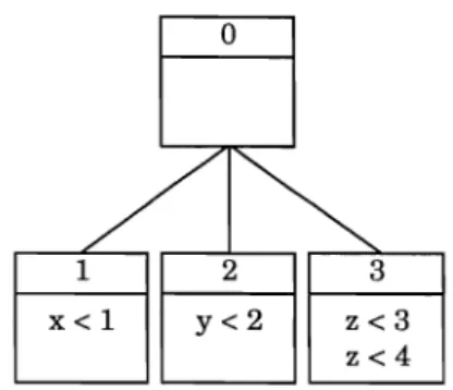
The branching scheme can best be illustrated on a small problem example. Assume that the set of activities {1,2,3,4} creates a resource conflict at decision point m and that the minimal delaying set is { { 1 }, {2}, {3,4} }. Assume that activity x is the earliest finishing activity among 2, 3 and 4, that activity y is the earliest finishing activity among the activities J, 3 and 4 and that activity Z is the earliest finishing
activity among the activities J and 2. The resulting delaying alternatives are represented in Figure l.
The operator '<' denotes a temporal constraint, i.e. a delay up to the earliest finishing time of an activity in progress that does not belong to a delaying alternative.
The delayed activities are removed from the partial schedule and the set of activities in progress, and the algorithm continues by computing a new decision point. The search process continues until the dummy end activity has been scheduled. Every time such a complete schedule has been found,
backtracking occurs: a new delaying alternative is arbitrarily chosen from the set of delaying
alternatives left, and branching continues from that node. When level zero is reached in the search tree, the search process is completed.
0
/
~
1 2 3
x<l y<2 z<3
z<4 Figure 1. Minimal delaying alternatives
Two dominance rules are used to prune the search tree. The first one is a variation of the
well-known left-shift dominance rule, and can be stated as follows:
Theorem 3. If the delay of the delaying alternative at the previous level of the branch-and-bound tree forced an activity i to become eligible at time m,
if
the current decision is to start activity i at time m andif
activity i can be left-shifted without violating the precedence or resource constraints (because activities in progress were delayed), then the corresponding partial schedule is dominated.The second dominance rule is based on the concept of a cutset. At every time instant m a cutset
Cm is defined as the set of unscheduled activities for which all predecessor activities belong to the partial schedule Psm · The proof of the following theorem can be found in Demeulemeester (1992) and Demeulemeester and Rerroelen (1992):
Theorem 4. Consider a cutset Cm at time m which contains the same activities as a cutset Ck ' which
was previously saved during the search of another path in the search tree.
If
time k was not greater than time m andif
all activities in progress at time k did not finish later than the maximum of m and the finish time of the corresponding activities in PSm , then the current partial schedule PSm is dominated.The original DR-procedure has been tested with three lower bounding rules. The well-known
remaining critical path length bound LBO and critical sequence lower bound LBI (Stinson et al. 1978) are supplemented by an extended critical sequence lower bound LB2 which is computed by repetitively looking at a path of unscheduled, non-critical activities in combination with a critical path. The LB2
calculation starts by calculating the Stinson critical sequence lower bound. This allows to determine which activities cannot be scheduled within their slack time. Subsequently, all paths consisting of at least two unscheduled, non-critical activities, which start and finish with an activity that cannot be scheduled within its slack time, are constructed. A simple type of dynamic programming then allows for the calculation of the extended critical sequence bound for every non-critical path.
Subsequent research revealed that LBO outperformed the critical sequence lower bounds LBI and
LB2, when used in combination with the cutset dominance pruning rule. As a result, both LBI and LB2
have been removed from the procedure. Moreover, Mingozzi et al. (1995) have introduced a new lower bound LB3, based on a new mathematical formulation for the RCPSP and implemented by using a heuristic for solving a set packing problem. Demeulemeester and Rerroelen (1996d) have incorporated their own version of LB3 in the new DR-procedure based on the following heuristic. For each activity
iEA they determine its possible companions, i.e., the activities with which it can be scheduled in parallel, respecting both the precedence and resource constraints. All unscheduled activities i with a non-zero duration are then entered in a list L in non-decreasing order of the number of companions (non-increasing duration as a tie-breaker). The following procedure then yields a lower bound, LB3, for the partial schedule under consideration:
LB3:= the earliest completion time of the activities in progress; while list L not empty do
Take activity j on top of list L and determine its duration dj ; LB3 := LB3 + d;
J
Remove activity j and its companions from list L; enddo.
It is clear that other (more computationally intensive) heuristics can be used to calculate the lower bound LB3. The procedure described here is very fast and offers an excellent trade-off between tightness of the bound and the required computational effort. It generally improves the critical path lower bound, LBO, if there are pairs of activities that can be scheduled in parallel taking into consideration the precedence constraints only, but cannot be scheduled in this manner if resource constraints are taken into consideration.
In addition to the removal of LBI and LB2 and the possibility to use both LBO and LB3, the DH1-procedure is the result of two additional changes, which have been made in order to gain on speed and to exploit the power of modern 32-bit compiler architecture. The major change has to do with a new coding scheme for the cutset dominance rule. Being limited to matrices of at most 64 Kb, the original DOS-version of the DH-procedure used four matrices for coding the dominance rule. Two matrices of 64 Kb were used to store cutsets with the necessary information to apply the dominance rule and two matrices of 16 Kb contained the pointers to the cutsets listed in the two 64 Kb matrices. The flat memory model of 32-bit programming, which allows for more efficient memory addressing and increased usable memory size, makes it possible to implement the cutset dominance rule using only two matrices: one very large cutset matrix contains the cutsets with the additional information, while a second matrix of 256 Kb was used to store the pointers to the cutsets in the cutset matrix. This implementation has two important advantages: more cutsets can be saved (increasing the impact of the cutset dominance rule) and the code becomes simpler (improving the speed of its application). A second change involved merging different resource types into one global resource type. This change became possible because integers automatically consist of 32 bits when 32-bit programming is used. Using, for instance, 8 bits for every resource type allows to combine four resource types into one 32-bit integer representing one global resource type. Combining several resource types into one (or a few) global resource type(s) leads to a definite speed-up of the code.
The logic of the DH2-procedure differs from the logic used by DHI in the additional use of a new resource-based lower bound, and an improved immediate scheduling rule for putting eligible activities in progress, which replaces the rules described in Theorem 1 and Theorem 2. Other differences boil down to the use of 64 Mb of addressable memory, a more efficient coding of the cutset dominance rule
(involving a more effective way of storing efficient cutsets), some preprocessing and additional code polishing.
2.3 Problem complexity and the prediction of the computational requirements
As mentioned earlier, extensive computational experience with the optimal solution procedures for the RCPSP has been gained on different test sets of problem instances: the 110 Patterson problem set and the 480 KSD problem set. Ideally such a set should span the full range of complexity, from very easy to very hard problem instances. The generation of easy and hard problem instances, however, appears to be a very difficult task which heavily depends on the possibility to isolate the factors that precisely determine the computing effort required by the solution procedure used to solve a problem, and the calibration of the scale that characterizes such effort. The 110 test problems, assembled by Patterson (1984), are a collection from different sources and have not been generated by using a controlled design of specified problem parameters. The 480 KSD instances used by Kolisch et al. (1995) have been generated using the problem generator ProGen through the use of a controllable set
of specified problem parameters. Recently, ProGen has been used to generate thousands of additional
test instances, which have made it possible to gain additional important insight in the factors that seem to determine the complexity (in terms of the required computation time) of an RCPSP instance.
2.3.1 The relation between problem hardness and topological network structure
De Reyck and Herroelen (1996a) have generated five sets of 1000 RCPSP instances, each with 25 activities, a maximum number of predecessors, resp. successors set to 25, 3 resource types with a constant availability of 6 units, resource requirements drawn from the uniform distribution in the range [1,5], and activity durations drawn from the uniform distribution in the range [1,10]. In each of the five sets, the coefficient of network complexity, CNC, is set at a different value, varying from 1.5 in the first
set to 2.5 in the fifth. Each RCPSP instance was then solved using the DH-procedure.
The CNC is undoubtedly one of the most popular 'measures of network complexity'. Introduced by Pascoe (1966) for activity-on-the-arc networks, and simply defined as the ratio of the number of arcs over the number of nodes, the measure has been adopted in a number of studies since then (Davis 1975, Talbot 1982, Patterson 1984, Kurtulus and Narula 1985, and Kolisch et al. (1995)). As observed by Kolisch et al. (1995), in the activity-on-the-node representation, 'complexity' has to be understood in the way that for a fixed number of activities (nodes), a higher complexity results in an increasing number of arcs and therefore ina greater connectedness of the network. A number of studies in the literature (Alvarez-Valdes and Tamarit 1989, Kolisch et al. 1995) seem to confirm that problems become easier with increasing values of the CNC, which makes the use of the CNC somewhat confounding (Elmaghraby and Herroelen (1980) already questioned the use of the CNC). Both Alvarez-Valdes and Tamarit (1989) and Kolisch et al. (1995) observe a negative correlation between the CNC and the required solution time for solving an RCPSP instance. De Reyck and Herroelen (1996a) reach the conclusion that it is very ambiguous to attach all explanatory power of problem complexity to the CNC. They observed a positive correlation between the CNC and the so-called complexity index, CI.
The complexity index, CI, is defined as the reduction complexity (Bein et al. 1992); i.e. the minimum number of node reductions sufficient (along with series and parallel reductions) to reduce a two-terminal acyclic network to a single edge. The CI-values for the instances used in the experiment range from 9 to 21. The authors found that the CI plays an important role in predicting the required computing effort for solving an RCPSP instance (the higher the CI, the easier the RCPSP instance) and that the CI outperforms the CNC as a measure of network complexity (the CNC explains nothing extra above what is already explained by the CNC). The reason for the strong explanatory power attributed to the CNC in previous experiments performed in the literature is probably due to the fact that when the CNC was varied, other parameters (such as the CI) were varied also, which led to problems with significant differences in 'complexity'.
In a subsequent experiment, De Reyck (1995b) again used ProGen to generate 4200 instances (25
activities, maximum number of start, resp. finish activities set to 5, maximum number of predecessors, resp. successors set to 25, 3 renewable resource types, activity durations and resource requirements drawn uniformly from the interval [1,10], CNC ranging from 1.2 to 2.5 and CI ranging from 1 to 17). Each instance was then solved using the DHI procedure. Again the CI was found to have a strong impact on the required processing time whereas the CNC had no impact at all. In addition, Schwindt's conjecture (Schwindt 1995) could be confirmed that an estimator for the so-called restrictiveness,
namely RT, is a good network complexity measure. De Reyck (l995b) has shown that RT is actually identical to the order strength, OS, one of the best complexity measures for generating and evaluating
assembly line balancing problems (see De Reyck and Herroelen 1995). OS is defined as the number of precedence relations, including the transitive ones, divided by n(n-l)l2, where n denotes the number of
activities (Mastor 1970). It is sometimes referred to as the density (Kao and Queranne 1992) and
actually equal to 1 minus the flexibility ratio, defined by Dar-EI (1973) as the number of zero entries in
the precedence matrix divided by the total number of matrix entries. Using values of RT ranging from 0.15 to 0.70, De Reyck (1995b) reached the conclusion that RT absorbed the explanatory power of both the CNC and the CI, and that RT outperforms both measures.
2.3.2 The RCPSP and resource availability
De Reyck and Herroelen (1996a) have also tried to isolate the impact of the resource availability (or resource-constrainedness) on the required solution effort for solving the RCPSP. Elmaghraby and Herroelen (1980) conjectured that the relationship between the hardness of a problem (as measured by the CPU time required for its solution) and resource availability (scarcity) varies according to a bell-shaped curve. If resources are only available in extremely small amounts, there will be relatively little freedom in scheduling the activities. Hence, the corresponding RCPSP instance should be quite easy to solve. If, on the other hand, resources are amply available, the activities can be simply scheduled in parallel and the resulting project duration will be equal to the critical path length, leading again to a small computational effort.
Two of the best known parameters for describing resource availability (scarcity) that have been proposed in the literature are the resource factor and the resource strength. The resource factor, RF
(Pascoe 1966, Cooper 1976, Alvarez-Valdes and Tamarit 1989, Kolisch et al. 1995) reflects the average portion of resources requested per activity. If we have RF=I, then each activity requests all resources. RF=O indicates that no activity requests any resource. The resource strength, RS (Cooper 1976) is redefined by Kolisch et al. (1995) as
(ak -
r tin)j(rtax -
r tin ), whereak
is the toal availability of renewable resource type k, r tin = maxi=l, ...,n 'ik'
andrkmax
is the peak demand of resource type k in the precedence-based earliest start schedule. Hence, with respect to one resource the smallest resource availability is obtained for RS=O. For RS=I, the problem is no longer resource-constrained. In their experiments, Kolisch et al. (1995) conclude (in contradiction with Alvarez-Valdes and Tamarit 1989) that RS has the strongest impact on solution times: the average solution time continuously increases with decreasing RS. De Reyck and Herroelen (1996a), however, could not confirm the continuous increase of the required solution time with decreasing RS but found a bell-shaped relationship, in accordance with the conjecture of Elmaghraby and Herroelen (1980).Patterson (1976) defines the resource-constrainedness, RC, for each resource k as p/ak , where ak
is the availability of resource type k and Pk is the average quantity of resource k demanded when required by an activity. The arguments for using RC and not RS as a measure of network complexity are that (a) RC is a 'pure' measure of resource availability in that it does not yet incorporate information about the precedence structure of a network, and (b) there are occasions where RS can no longer distinguish between easy and hard instances while RC continues to do so (for details, we refer to De Reyck and Herroelen 1996a). Again, De Reyck and Herroelen (1996a) are able to confirm a bell-shaped relationship between the CPU time and RC.
2.4 Branch-and-bound procedures for solving the RCPSP: conclusions
The fundamental conclusions which can be drawn from the reviewed research on branch-and-bound schemes for the RCPSP can be summarized as follows:
(i) a depth-first branch-and-bound search strategy based on resolving resource conflicts by delaying minimal subsets of activities is a clear favourite for optimally solving RCPSP instances;
(ii) the cutset dominance rule ranks amongst the most effective dominance pruning rules, especially if a sufficient amount of memory (e.g. 24 Mb) can be used for storing the cutsets;
(iii) the use of easy to compute and effective lower bounds (e.g. LB3 and its possible variations; the new resource-based bound incorporated in DH2) has a strong impact on the computational cost; (iv) it is extremely important to exploit the trade-off between the strength of the bounds or dominance
rules used and the time required for their computation;
(v) truncated depth-first branch-and-bound procedures provide a suitable alternative to priority based heuristics such as MINSLK (the first solution obtained is often better than the one obtained by MINSLK; near-optimal solutions are obtained even if the truncated procedure is only allowed to run for a small amount of time, e.g. an average deviation on the 480 KSD problems of 0.575 %
(vi) sufficient attention should be devoted to efficient coding of the solution procedures used;
(vii) exploiting the full potential of 32-bit programming provided by recent compilers running on personal computer platforms such as Windows NT® and OS/2® may add considerably to the efficiency of the computer code used;
(viii) reproducable optimal benchmark results are available on the 110 Patterson problems and the 480 KSD problems. In order to avoid computational bias and to guarantee that procedures are validated on a relevant spectrum of problem complexity (the complexity of a problem instance is entwined to the procedure used to solve it), computational experience should be reported on the complete problem sets and should not be limited to selected problem subsets assumed to be "hard" or "easy".
3. The preemptive resource-constrained project scheduling problem (PRCPSP)
The PRepSp allows activities to be preempted at integer points in time; i.e., the fixed integer
duration di of an activity may be split inj = 1,2, ... ,di duration units. Each duration unitj of activity i is then assigned an integer finish time
f '.
The variablef
0 denotes the earliest time that an activity i can be'J "
started. As only finish-start relations with a time lag of zero are allowed,/; 0 equals the latest finish time
"
of all the predecessors of activity i. An activity i belongs to the set St of activities in progress in period
]t-l,t] if one of its duration units j = 1,2, ... ,di finishes at time t (i.e., if!;) = t). The PRCPSP can now be conceptually formulated as follows (Demeulemeester 1992):
mm fn,o subject to
fiA
Ji,j-l+
::;;
Ao
0I.
'ik ::;; ak iES,f ·
J, 0 for all (i, J') E HFl' J' i
=
1, ... , n; J'=
1, ... , dl• Ji, k=
1, ... , K; t=
1, ... , fn,o[5]
[6]
[7]
[8]
[9]
The objective function (Eq. 5) minimizes the project length by minimizing the earliest start time of the dummy end activity which by assumption has a duration of O. Eqs. 6 assure that all precedence relations are satisfied: the earliest start time of an activity j cannot be smaller than the finish time of the last unit of duration of its predecessor i. Eqs. 7 specify that the finish time for every unit of duration of an activity has to be at least one time unit larger than the finish time for the previous unit of duration. Activity 1 is assigned an earliest start time of 0 through Eq. 8, while Eqs. 9 stipulate the resource constraints.
Slowinski (1980) and Weglarz (1981) have presented optimal solution procedures for the case of continuous processing times for the different activities. Davis and Heidorn (1971) developed an implicit
enumeration scheme based on the splitting of activities in unit duration tasks. Kaplan (1988, 1991) presents a dynamic programming formulation and suggests a solution by a reaching procedure.
The DH-procedure has been extended to the PRCPSP (Demeulemeester and Herroelen 1996b). In order to do so it is assumed that only two dummy activities exist in the project: the dummy start and the dummy end. This is caused by the time incrementing scheme used, which augments the decision points by one time unit at a time. In addition a distinction is made between activities and subactivities. At the start of the procedure we create a new project network in which all activities are replaced by one or more subactivities. The dummy start and end activities are replaced by dummy start and end subactivities with a duration of O. All other activities are split into subactivities, their number being equal to the duration of the original activity, each having a duration of 1 and resource requirements that are equal to those of the original activity. Demeulemeester and Herroelen (1996b) prove that in order to solve the PRCPSP, it is sufficient to construct partial schedules by semi-active timetabling at the level of the subactivities.
An eligible activity is defined as an activity for which one of the subactivities is eligible. An
unfinished activity is an activity for which not all subactivities have been scheduled. Denote the z
unfinished subactivities of unfinished activity i at time t as ii' i2, ... , iz . We say that activity i is scheduled immediately at time t if all its remaining subactivities ix (x = l, ... ,z) are scheduled such that
fix = t + x.
Theorems 1 and 2 stated above for the RCPSP can now be extended in the following way.
Theorem 5. lffor a partial schedule PSm at time instant m there exists an eligible activity i that cannot
be scheduled together with any other unfinished activity j at any time instant m' ;;? m without violating the precedence or resource constraints, then an optimal continuation of PSm exists with all remaining
subactivities ii' i2, ... , iz of activity i scheduled immediately at time m.
The reader should notice that it is not necessary to check whether an activity is in progress or not at time m. The scheduling of an activity at the previous decision point does not imply that if that activity was not completed, the same activity should also be scheduled at the current decision point. The preemption condition allows to forget the scheduling decisions in previous periods and to consider only those possibilities implied by the set of eligible subactivities.
Theorem 6. lffor a partial schedule PSm at time instant m there exists an eligible activity i that can be scheduled together with only one other unfinished activity j at any time instant m' ;;? m without violating the precedence or resource constraints and
if
activity j is eligible, then an optimal continuation of PSm exists with all remaining subactivities of activity i scheduled immediately and withas many subactivities of activity j as possible scheduled concurrently with the subactivities of activity i.
The reader will have noticed that no test needs to be performed to check whether the remaining duration of activity j is larger than that of activity i. Indeed, if the remaining duration of activity j is larger, as many subactivities of activity j will be scheduled as there are unscheduled subactivities in
activity i. If, however, the remaining duration of activity j is smaller or equal, all remaining subactivities of activity j will be scheduled concurrently with those of activity i.
Demeulemeester and Herroelen (l996b), are able to prove the following dominance rule which very much resembles the cutset dominance rule stated earlier for the RCPSP.
Theorem 7. Consider a partial schedule PSm at time m. If there exists a partial schedule PSk that was previously saved at a similar time m and
if
PSm is a subset of PSk> then the current partial schedulePSm is dominated.
Demeulemeester and Herroelen (1996b) also show that it is sufficient to consider only minimal delaying alternatives in order to resolve resource conflicts. In addition, they have shown that all three lower bounds discussed earlier (LBO, LBI and LB2) remain applicable, at the trade-off of increased
computational requirements. Therefore, they only included LBO in the code. LB3, which is extendable
to the PRCPSP but was only developed very recently, could not be included at the time the code was written.
As was already mentioned before, the literature on the PRCPSP is almost void and very little computational experience is available. Demeulemeester and Herroelen (1996b) have programmed their procedure in Turbo C Version 2.0 for a personal computer IBM PS/2 Model 70. On the same 41 Patterson test problems used by Kaplan (1988, 1991) and using a similar PC running at 16 MHz, it finds the optimal solution in an average CPU time of 4.9863 seconds with a standard deviation of 9.2932 seconds, while the Kaplan code requires an average of 425 seconds and a standard deviation of 713 seconds, respectively. Using a personal computer IBM PS/2 running at 25 MHz, they have tested their algorithm on all 110 Patterson test problems. All problems could be solved within 5 minutes of CPU time, requiring an average of 6.8985 seconds and a standard deviation of 25.8149 seconds.
Demeulemeester (1992) has extended the code for the PRCPSP with variable resource availabilities. In that case, Theorems 5 and 6 no longer apply. A total of 107 out of the 110 Patterson test problems, modified by Simpson and Patterson (1996) to incorporate variable resource availabilities, could be solved on an average computation time of 12.6321 seconds and a standard deviation of 36.9071 seconds.
4. Project scheduling under generalized precedence relations
A lot of research efforts have been directed towards relaxing the strict precedence assumption of CPM/PERT. The resulting types of precedence relations are often referred to as MPM (Metra Potential Method) precedence constraints (Kerbosch and Schell 1975, Zhan 1994), precedence diagramming (Moder et al. 1983), time windows (Bartusch et al. 1988), minimal and maximal time lags (Brinkmann and Neumann 1994, Neumann and Schwindt 1995, Schwindt 1995, Franck and Neumann 1996, Neumann and Zahn 1996, Schwindt and Neumann 1996), and generalized precedence constraints (Wikum et al. 1994). In accordance with Elrnaghraby and Karnburowski (1992), we denote them as generalized precedence relations (GPRs) and distinguish between start-start (SS), start-finish (SF), finish-start (FS) and finish-finish (FF).
GPRs can specify a minimal or maximal time lag between any pair of activities. A minimal time lag specifies that an activity can only start (finish) when the predecessor activity has already started (finished) for a certain time period. A maximal time lag specifies that an activity should be started (finished) at the latest a certain number of time periods beyond the start (finish) of another activity.
4.1. The generalized resource-constrained project scheduling problem (GRCPSP)
Demeulemeester and Herroelen (1996a) have extended the DH-procedure to the case of minimal
time lags, activity release dates and deadlines and variable resource availabilities. The resulting problem, which they denote as the GRCPSP, can be conceptually formulated as follows:
mill
In
subject to Ii Ii Ii IiII
Ii -di d· ! 0 di Ii ::; hi+
+
+
+
~ L rkt ::; akt iES, where SSij ::; Ij SFij ::; Ij FSij ::; Ij FFij ::; Ij gi - d j - d jfor all (i, j) E HI
for all (i,j) E H2 for all (i,j) E H3 for all (i,j) EH4
i
=
1,2, ... ,ni
=
1,2, ... ,nk=I,2, ... ,K; t=I,2, ...
,/n
HI = set of pairs of activities indicating start-start relations with a time lag of SSij
H 2 = set of pairs of activities indicating start-finish relations with a time lag of SF ij
H 3 = set of pairs of activities indicating finish-start relations with a lag of FSij
H4 = set of pairs of activities indicating finish-finish relations with a lag of FF ij gi = ready time of activity i
hi = due-date of activity i
akt = availability of resource type k during period ]t-1,t]
[10]
[11]
[12][13]
[14] [15] [16] [17] [18]The objective function CEq. 10) is to minimize the project duration by minimizing the finish time of the unique dummy end activity n. Eqs. 11-14 ensure that the various types of precedence constraints are satisfied. Eq. 15 assigns the dummy start activity 1 a completion time of O. Eqs. 16 guarantee that the ready times are respected, while Eqs. 17 guarantee that no due-dates are violated. Eqs. 18 specify that the resource utilization during any time interval ]t-1,t] does not exceed the resource availability levels during that time interval for any of the resource types.
In order to extend the DH-procedure to the GRCPSP, all precedence constraints are converted to finish-start precedence relations using the following conversion formula:
FS' ..
IJ max{SS .. IJ -d. 1 ' SP.·-d·-d· FS·· FP..-d.} IJ 1 J ' IJ ' IJ J
[19]
The ready time gi of an activity i can easily be transformed into a finish-start relation between the dummy start activity 1, which starts and finishes at time 0, and activity i itself:
FS "Ii [20]
Coping with deadlines hi is somewhat more involved. For every activity j a latest allowable start time Is. has to be computed such that whenever this activity j is delayed to start later than Is., the
J J
deadline of this activity or of one of its direct or indirect successors is exceeded even if all subsequent activities were scheduled as soon as possible without considering the resource constraints. Consequently, if during the branch-and-bound procedure an activity j is assigned an early start time Sj that exceeds its latest allowable start time ISj' backtracking can occur as no feasible solution can be found by continuing the search from this partial schedule.
As before, St is defined as the set of activities in progress during the time interval ]t-l,t], PSt as the partial schedule which contains the set of activities that have been assigned a finish time at time t, and the cutset Ct as the set of all unscheduled activities whose predecessors all belong to the partial schedule PSt" The eligible set Et then denotes the set of all activities that belong to the cutset Ct and that
can start at time t. The precise time instant at which these sets are defined will be clear from the context, hence, the subscripts will be omitted for simplicity of notation.
The search process starts by adding the dummy start activity 1 to Sand P S with a finish time
II
=0. All activities i that have activity 1 as a single predecessor are added to the cutset and are assigned an early start time, based on the precedence relations FS" Ii (which include the ready times). The next decision point m is then computed as the smallest early start time of any activity in the cutset. The activities in the cutset that can start at time m are added to the eligible set E. All activities in S that complete before time m are deleted from S and all activities in E are scheduled: they are added to SandPS and are assigned a finish time that equals the sum of the decision point m and the duration of the activity involved. The cutset is updated. If due to resource constraints it is impossible to schedule all activities in E concurrently, a resource conflict occurs. Such a conflict will produce a new branching in the branch-and-bound tree at level p: the branches describe ways to resolve the resource conflict; i.e., decisions about which combinations of activities are to be delayed.
A delaying alternative D q is defined as the set of activities that belong to S, the delay of which would resolve the resource conflict that occurred at level p of the solutions tree and for which it holds that if an activity belongs to D q all its direct and indirect successors that belong to S are also included in D q' In order to simplify the construction process of the delaying alternatives, a precedence relation is
added for every activity that can be partially overlapped with one of its indirect successors. As such, only the direct successors need to be examined in order to satisfy the second condition. The delaying
set D(p) then consists of all possible delaying alternatives D q that resolve the resource conflict at level p
of the branching tree. For each delaying alternative D the delaying point w is computed as the earliest q q time at which either the resource availability changes, or an activity that belongs to (S-D ) finishes, or
q
one of the unscheduled activities that has no predecessor in D q could finish if all unscheduled activities were scheduled as soon as possible. A precedence based lower bound Lq is then calculated by adding
the maximal remaining critical path length of any of the activities that belong to D q to the delaying
point wq . The delaying alternative with the smallest lower bound is chosen (ties are broken arbitrarily)
and these activities are removed from Sand PS (as well as all completed successors of one of these activities). All other delaying alternatives are stored for backtracking purposes. The cutset is updated and the process of constructing the eligible set, adding it to Sand PS and branching whenever resource conflicts occur is repeated until a solution to the problem is found or until it can be shown that by branching from this node only infeasible solutions or dominated solutions could be generated. When this happens the procedure backtracks.
Demeulemeester and Herroelen (1996a) prove that the partial schedules may be constructed by semi-active timetabling. In addition they show that it is sufficient to consider only minimal delaying alternatives in order to resolve a resource conflict. Last but not least, they extend the left-shift and cutset dominance rules. They also show that the critical sequence bound LBl and the extended critical sequence bound LB2 cannot be extended, leaving the remaining critical path length LBO as a possible lower bound (again LB3 can be extended to the GRCPSP but was not yet known when writing the code).
The literature on the GRCPSP is very limited and a standard set of test problems has not yet been established. Demeulemeester and Herroelen (1996a) have coded the GDH-procedure in Turbo C Version 2.0 for IBM PS/2 computers with 80486 processor operating at 25 MHz (or compatibles). The procedure was then tested on the 110 Patterson test problems as modified by Simpson and Patterson (1996) to incorporate variable resource availabilities. The GDH-procedure could find the optimal solution for all 110 problems with constant resource availabilities in an average of 0.1446 seconds and a standard deviation of 0.3027 seconds. For the problems with variable resource availabilities, the GDH-procedure, when given a time limit of 10 minutes, could optimally solve 109 out of the 110 problems to optimality in an average CPU time of 8.1065 seconds (vis-a-vis 100.85 seconds required on average by Simpson's serial procedure to solve 97 problems and 96.63 seconds required on average by Simpson's parallel procedure to solve 98 problems) and a standard deviation of 57.775 seconds (vis-a-vis 199.62 seconds for Simpson's serial procedure and 195.90 seconds for Simpson's parallel procedure). When the code is allowed to run to completion, all problems are solved in an average of 60.1561 seconds and a standard deviation of 548.9009. As such, the GDH-procedure seems to be a very efficient and