OpenBU http://open.bu.edu
Theses & Dissertations Boston University Theses & Dissertations
2018
Safety-aware apprenticeship
learning
https://hdl.handle.net/2144/30743
COLLEGE OF ENGINEERING
Thesis
SAFETY-AWARE APPRENTICESHIP LEARNING
by
WEICHAO ZHOU
B.S., Fudan University, 2012
Submitted in partial fulfillment of the
requirements for the degree of
Master of Science
2018
First Reader
Wenchao Li
Assistant Professor of Electrical and Computer Engineering Assistant Professor of Systems Engineering
Second Reader
Brian Kulis
Assistant Professor of Electrical and Computer Engineerings Assistant Professor of Systems Engineering
Assistant Professor of Computer Science
Third Reader
Yannis Paschalidis
Professor of Electrical and Computer Engineering Professor of Systems Engineering
I want to express my deepest appreciation to my advisor, Professor Wenchao Li. During my two-year master’s studies, he has always been a great mentor for me. He set an example of excellence as a researcher, instructor and role model. My experiences in his group have always been rewarding. Conducting researches under his guidance motivates me to refine my skills and set a high standard for myself. I cherish this opportunity for professional and personal development that he has provided me.
I would like to thank my thesis committee members for providing me support through this process. Your suggestions and feedback have been invaluable for me.
I also want to thank our department for providing me with such an open and resourceful environment. I’m so glad that I will be able to continue enjoying my time here as a PhD student.
Last but not least, I can not tell how grateful I am to my parents. I would not have been here without your encouragement. You believe in me and always want the best for me. You are oceans away, yet your love is close.
WEICHAO ZHOU
ABSTRACT
It is well acknowledged in the AI community that finding a good reward function for reinforcement learning is extremely challenging. Apprenticeship learning (AL) is a class of “learning from demonstration” techniques where the reward function of a Markov Decision Process (MDP) is unknown to the learning agent and the agent uses inverse reinforcement learning (IRL) methods to recover expert policy from a set of expert demonstrations. However, as the agent learns exclusively from obser-vations, given a constraint on the probability of the agent running into unwanted situations, there is no verification, nor guarantee, for the learnt policy on the sat-isfaction of the restriction. In this dissertation, we study the problem of how to guide AL to learn a policy that is inherently safe while still meeting its learning objective. By combining formal methods with imitation learning, a Counterexample-Guided Apprenticeship Learning algorithm is proposed. We consider a setting where the unknown reward function is assumed to be a linear combination of a set of state features, and the safety property is specified in Probabilistic Computation Tree Logic (PCTL). By embedding probabilistic model checking inside AL, we propose a novel
counterexample-guided approach that can ensure both safety and performance of the learnt policy. This algorithm guarantees that given some formal safety specification defined by probabilistic temporal logic, the learnt policy shall satisfy this specifica-tion. We demonstrate the effectiveness of our approach on several challenging AL scenarios where safety is essential.
1 Introduction 1
1.1 Contributions . . . 3
1.2 Related Work . . . 3
1.3 Outline . . . 5
2 Background 6 2.1 Markov Decision Process . . . 6
2.2 Probabilistic Model Checking . . . 8
2.3 Counterexample . . . 10
3 Counterexample-Guided Apprenticeship Learning 12 3.1 Motivating example . . . 12
3.2 A Framework for Safety-Aware Learning . . . 15
3.3 An Algorithm for Counterexample-Guided Apprenticeship Learning . 18 3.4 Convergence Analysis . . . 23
3.5 Summary and Discussion . . . 25
4 Experiments 26 4.1 Navigation in Grid World . . . 26
4.2 Cart-Pole from OpenAI Gym . . . 28
4.3 Mountain-Car from OpenAI Gym . . . 30
4.4 Discussion . . . 33
5 Conclusions 34
5.2 Future Work . . . 35
References 37
Curriculum Vitae 41
4.1 Average runtime per iteration in seconds. . . 27 4.2 In the cart-pole environment,higheraverage steps mean better
perfor-mance. The safest policy is synthesized using PRISM-games. . . 29 4.3 In the mountain-car environment, lower average steps mean better
performance. The safest policy is synthesized via PRISM-games. . . . 32
3·1 Navigation task in gridworld . . . 13
3·2 Counterexample-Guided Apprenticeship Learning . . . 16
3·3 Max margin principle . . . 17
4·1 Reward mappings of gridworld for different safety threshold . . . 27
4·2 The cartpole environment . . . 28
4·3 The mountaincar environment . . . 31
AI . . . Artificial Intelligence AL . . . Apprenticeship Learning
CEGAL . . . Counterexample-Guided Apprenticeship Learning CEGIS . . . Counterexample-Guided Inductive Synthesis CEX . . . Counterexample
IRL . . . Inverse Reinforcement Learning
PCTL . . . Probabilistic Computational Tree Logic Safe-AL . . . Safety-Aware Apprenticeship Learning
Chapter 1
Introduction
AI safety has been one of the main factors limiting the deployment of artificial intelligence (Bundy, 2016). As AI technologies are gaining rapid progress in a diversity of areas, such as computer vision (Krizhevsky et al., 2012), video games (Mnih et al., 2015), and autonomous driving (Levinson et al., 2011), concerns about unintended consequences of widespread adoption have been raised. When exposed to the full complexity of the human environment, an AI agent should not only be able to finish the task assigned by human but also ensure that its probability of performing unsafe actions is at least below some acceptable threshold. This is especially significant in safety critical areas. As highlighted in (Amodei et al., 2016), if the objective function of an AI agent is wrongly specified, then maximizing that objective function may lead to harmful results. In addition, if an agent focuses only on accomplishing a specific task and ignore other aspects, such as safety constraints, of the environment, it may also perform unsafe behavior. But among various reasons why an agent learns an unsafe policy, the direct and intuitive cause is that the agent lacks for awareness of unsafe situations.
In this dissertation, we focus on the safety problems when AI learns from human demonstration and explore the following thesis:
Given a safety specification, by learning from human demonstration with a verification-guided algorithm, an agent can ensure the safety of apprenticeship learning while re-taining its performance.
Apprenticeship learning (AL)approach developed by Abbeel and Ng (Abbeel and Ng, 2004) is one form of learning from demonstration where an agent tries to re-cover an expert’s strategy by observing and learning from the expert’s demonstration. This approach uses inverse reinforcement learning (Ng and Russell, 2000) technique in which it is assumed that expert makes decisions optimally in the environment. Apprenticeship Learning bypasses the explicit search of reward function as in rein-forcement learning and directly recovers the expert’s policy by matching the features of the expert’s demonstration. However, the expert often can only demonstrate how the task works but not how the task may fail. This is because failure may cause irrecoverable damages to the system such as crashing a vehicle. In general, the lack of “negative examples” can cause a heavy bias in how the learning agent constructs the reward estimate. In fact, even if all the demonstrations are safe, the agent may still end up learning an unsafe policy.
Probabilistic Model Checking is a range of techniques calculating the like-lihood of the occurrence of certain events during the execution of a probabilistic system (Kwiatkowska et al., 2002). Considering a safety specification expressed in probabilistic computation tree logic (PCTL) (Hansson and Jonsson, 1994), we employ a verification-in-the-loop approach by embedding probabilistic model check-ing (Kwiatkowska et al., 2002) as a safety checkcheck-ing mechanism inside the learncheck-ing phase of AL. Inspired by the work on formal inductive synthesis (Jha and Seshia, 2017) and counterexample-guided inductive synthesis (Solar-Lezama et al., 2006), we incorporate formal verification in apprenticeship learning and propose a frame-work that uses the verification results to inductively improve the learnt policy. More specifically, when a learnt policy does not satisfy the PCTL formula, we leverage counterexamples generated by the model checker to steer the policy search in AL. In essence, counterexample generation can be viewed as supplementing negative
exam-ples for the learner. Thus, the learner will try to find a policy that not only imitates the expert’s demonstrations but also stays away from the failure scenarios as captured by the counterexamples.
1.1
Contributions
In summary, we make the following contributions in this thesis.
• We propose a novel framework for incorporating formal safety guarantees in learning from demonstrations.
• We develop a novel algorithm called CounterExample Guided Apprenticeship Learning (CEGAL) that combines probabilistic model checking with the opti-mization based approach of apprenticeship learning.
• We demonstrate that the proposed approach can guarantee safety for a set of case studies and attain performance comparable to using apprenticeship learning alone.
1.2
Related Work
A taxonomy of AI safety problems is given in (Amodei et al., 2016) where the issues of misspecified objective or reward and insufficient or poorly curated training data were highlighted. There have been several efforts attempting to address these issues from different angles. The problem of safe exploration is studied in (Moldovan and Abbeel, 2012) and (Held et al., 2017). In particular, the latter work proposes to add a safety constraint on amount of damage, to the optimization problem so that the optimal policy can maximize the reward without violating the limit on the expected damage. An obvious shortcoming of this approach is that actual failures will have to occur so that the constraint can be properly decided.
Formal methods have been applied to the problem of AI safety. In (Gillulay and Tomlin, 2011), the authors propose to combine machine learning and reachability analysis for dynamical models to achieve high performance and guarantee safety. In (Sadigh et al., 2014), the authors propose to use formal specification to synthesize a control policy for reinforcement learning. Recently, the problem ofsafe reinforcement learning was explored in (Alshiekh et al., 2017) where a monitor (called shield) is used to enforce temporal logic properties by providing a list of safe actions each time the agent makes a decision so that the temporal property is preserved. In (Junges et al., 2016), the authors also propose an approach for controller synthesis for rein-forcement learning by using an SMT-solver is used to find a scheduler (policy) so that it satisfies both a probabilistic reachability property and an expected cost property. In (Mason et al., 2017), a so-called abstract Markov decision process (AMDP) model of the environment is first built and PCTL model checking is then used to check the satisfiability of safety specification. Our work is similar to these in spirit in the application of formal methods. However, while the concept of AL is closely related to reinforcement learning, an agent in the AL paradigm needs to learn a policy from demonstrations without knowing the reward function. A related safety problem in verification is the faithfulness of the model when it is learned from data. In (Puggelli et al., 2013), the authors propose a convex-MDP model for capturing uncertainties in the transition probabilities of an MDP as convex sets and propose a polynomial-time algorithm for verifying PCTL properties on these convex-MDPs.
Among imitation or apprenticeship learning methods, margin based algorithms (Abbeel and Ng, 2004), (Ng and Russell, 2000), (Ratliff et al., 2006) try to maximize the margin between the expert’s policy and all learnt policies until the one with the smallest margin is produced. The apprenticeship learning algorithm in (Abbeel and Ng, 2004) was largely motivated by the support vector machine (SVM). Our algorithm
makes use of this observation when using counterexamples to steer the policy search process. Recently, the idea of learning from failed demonstrations started to emerge. In (Shiarlis et al., 2016), the authors propose an IRL algorithm that can learn from both successful and failed demonstrations. It is done by reformulating maximum en-tropy algorithm in (Ziebart et al., 2008) to find a policy that maximally deviates from the failed demonstrations while approaches the successful ones as much as possible. However, this entropy-based method requires obtaining many failed demonstrations and can be very costly in practice.
Finally, our approach is inspired by the work on formal inductive synthesis (Jha and Seshia, 2017) and counterexample-guided inductive synthesis (CEGIS) (Solar-Lezama et al., 2006). These frameworks typically combine a constraint-based syn-thesizer with a verification oracle. In each iteration, the agent refines her hypothesis (i.e. generates a new candidate solution) based on counterexamples provided by the oracle. Our approach can be viewed as an extension of CEGIS where the objective is not just functional correctness but also meeting certain learning criteria.
1.3
Outline
The rest of the thesis is organized as follows. Chapter 2 reviews background in-formation on apprenticeship learning and PCTL model checking. Chapter 3.1 de-fines the safety-aware apprenticeship learning problem. Chapter 3.2 illustrates the counterexample-guided learning framework and gives an overview of our approach. Chapter 3.3 and 3.4 describes the proposed algorithm in detail. Chapter 4 presents a set of experimental results demonstrating the effectiveness of our approach.
Chapter 2
Background
2.1
Markov Decision Process
Definition 2.1.1. Markov Decision Process (MDP) is a tuple (S, A, T, γ, s0,
R), where S is a finite set of states; A is a set of actions; T : S×A×S → [0,1] is a transition function describing the probability of transitioning from one state s∈S
to another s0 ∈S by taking action a ∈A in state s; R: S →R is a reward function which maps each state s ∈ S to a real number indicating the reward of being in state s; s0 ∈S is the initial state; γ ∈ [0,1) is a discount factor which describes the desirability of the future rewards.
A policyπfor an MDPM induces a Discrete-Time Markov Chain (DTMC)Mπ =
(S, Tπ, s0), whereTπ :S×S →[0,1] is the probability of transitioning from a state s to another state in one step. By making a sequence of decisions by following policy
π, the agent shall traverse a trajectory τ = st0
Tπ(st0,st1)>0
−−−−−−−−→ st1
Tπ(st1,st2)>0
−−−−−−−−→st2, ..., is a sequence of states where sti ∈ S. The accumulated reward of such trajectory τ is
∞
P i=0
γiR(s
ti). The value functionVπ :S →Rmeasures the expectation of accumulated
reward E[
∞
P i=0
γiR(s
ti)] starting from a state s and following policy π.
According to (Bellman, 1957), a policy π is optimal for MDP M if:
∀s∈S, π(s)∈argmax a∈A
X
s0∈S
T(s, a, s0)Vπ(s0) (2.1)
Inverse reinforcement learning (Ng and Russell, 2000) assumes that a learning agent is provided with a set of m trajectoriesE ={τ0, τ1, ..., τm−1} from expert. The goal is to find a function R that can generate optimal behavior similar to E.
Apprenticeship learning (Abbeel and Ng, 2004) aims at producing a policy which performs almost as well as the expert without guaranteeing to recover the reward function. It is assumed that reward function is the result of linear combination
R(s) = ωTf(s), where f : S → [0, 1]k is a vector of feature functions on S and ω ∈ [0,1]k ∧ ||ω||
2 ≤ 1, is a weight vector. Feature function f is known by both expert and the learning agent. Given some weight vectorω, its corresponding reward function R is known and optimal policy π can be solved. The expected value of the initial state s0 can be expressed as:
Vπ(s0) = Eπ[ ∞ X i=0 γtR(sti)|st0 =s0] = Eπ[ ∞ X i=0 γtωTf(sti)|st0 =s0] = ωTEπ[ ∞ X i=0 γtf(sti)|st0 =s0] (2.2) Defineµπ =Eπ[ ∞ P i=0
γtf(sti)|st0 =s0] as the expected features of policy π. Given a policy π, then µπ can be solved through Monte Carlo method, or value iteration, or
linear programming. If expert has a weight vector ωE and a policy πE, the expected
features of expert’s policyµE can be expressed in the same way. However, practically only a limited amount of demonstrations will be provided by the expert. Define ˆµE
as the expected features of expert’s m trajectories. If m is large enough, µE can be
approximated by ˆµE. E[ i=m X i=1 X s(tji)∈τi γjR(s(tji))] =E[ i=m X i=1 X s(tji)∈τi γjωTf(st(ji))] = ωTE[ i=m X i=1 X s(tji)∈τi γjf(s(tji))] = ωTµEˆ (2.3)
The algorithm proposed by Abbeel and Ng (Abbeel and Ng, 2004) starts with a random policy π0 and its expected features µπ0. Assuming that in iteration i, a set of i candidate policies Π = {π0, π1, ..., πi−1} and their corresponding expected
features{µπ|π ∈Π}have been found, the algorithm solves the following optimization problem. δ= max ω minπ∈Π ω T (ˆµE−µπ) s.t.||ω||2 ≤1 (2.4) The optimal ω is used to find the corresponding optimal policy πi and the expected
featuresµπi. Ifδ≤, then the algorithm terminates andπiis produced as the output.
Otherwise, µπi is added to the set of features for the candidate policy set Π and the
algorithm continues to the next iteration.
2.2
Probabilistic Model Checking
Probabilistic model checking can be used to verify properties of a stochastic system such as “is the probability that the agent reaches the unsafe area within 10 steps smaller than 5%?”. Probabilistic Computation Tree Logic (PCTL) (Hansson and Jonsson, 1994) allows for probabilistic quantification of those properties. The syntax of PCTL includes state formulas and path formulas (Kwiatkowska et al., 2002). A state formula φ asserts property of a single state s ∈ S whereas a path formula ψ
asserts property of a trajectory.
φ ::= true | l | ¬φi |φi∧φj |Pnop∗[ψ] (2.5)
ψ ::= Xφ | φ1U≤kφ2 |φ1Uφ2 (2.6)
where l ∈ AP is an atomic proposition; on∈ {≤,≥, <, >}; Ponp∗[ψ] means that the probability of generating a trajectory that satisfies formula ψ is on p∗. Xφ asserts that the next state after initial state in the trajectory satisfies φ; φ1U≤kφ2 asserts that φ2 is satisfied in at most k transitions and all preceding states satisfy φ1; φ1Uφ2 asserts that φ2 will be eventually satisfied and all preceding states satisfy φ1.
and DTMC:
s |= true iff state s∈S (2.7)
s |= a iff a∈L(s) (2.8)
s |= φ iff state s satisfies state formula φ (2.9)
s |= ¬φ iff s|=φ is false (2.10)
s |= φ1∧φ2 iff s|=φ1 and s|=φ2 (2.11)
s |= Pnop∗(ψ) iff P rob(s, ψ)onp∗ (2.12)
The satisfaction relation |= between trajectory τ and path formula ψ is defined as below:
τ |= ψ iff τ satisfiesψ (2.13)
τ |= φ1U≤kφ2 iff ∃j ≤k, τ(stj)|=φ1∧ ∀0≤i≤j, τ(sti)|=ψ (2.14)
τ |= φ1W≤kφ2 iff τ |=φ1U≤kφ2 or ∀i≤k, sti |=φ1) (2.15)
In this thesis a third-party probabilistic model checking tool, PRISM (Kwiatkowska et al., 2002), is used. It can take a description of a system, which is a DTMC in this dissertation, with a set of PCTL specifications as inputs, then answers which states of the system satisfy each specification. This is a symbolic model checker (Fujita et al., 1997) which uses binary decision diagram (BDD) and multi-terminal BDDs (MTB-DDs) as the underlying data structures. The tool reduces the verification problem to reachability-based computation and numerical calculation. The data structures can help the tool perform efficient and fast computation on large, structured mod-els (Kwiatkowska et al., 2002).
A policy can also be synthesized by using model checking tool to solve the objective
min
the satisfiability of P≤p∗[ψ]. This problem can be solved by linear programming or policy iteration (and value iteration for step-bounded reachability) (Kwiatkowska and Parker, 2013).
2.3
Counterexample
One major strength of probabilistic model checking techniques is to generate coun-terexamples in case a temporal logic property is violated (Han et al., 2009). Coun-terexample can be viewed as a proof of the violation. In this thesis, it is used as demonstrations of unsafe behaviors.
In addition to the satisfaction relations in PCTL semantics, |=min denotes the
minimal satisfaction relation (Han et al., 2009) between τ and ψ. Defining pref(τ) as the set of all prefixes of trajectoryτ including τ itself, then τ |=min ψ iff (τ |=ψ)∧
(∀τ0 ∈pref(τ)\τ, τ0 2ψ). For instance, ifψ =φ1U≤kφ2, then for any finite trajectory
τ |=min φ1U≤kφ2, only the final state in τ satisfiesφ2. LetP(τ) be the probability of transitioning along a trajectory τ and let Γψ be the set of all finite trajectories that
satisfy τ |=min ψ, the value of PCTL property ψ is defined as P=?|s0[ψ] =
P τ∈Γψ
P(τ). For a DTMC Mπ and a state formula φ =P≤p∗[ψ], Mπ |=φ iff P=?|s
0[ψ]≤p
∗.
There can be different counterexamples for one formula. LetP(Γ) = P τ∈Γ
P(τ)≤p∗
be the sum of probabilities of all trajectories in one set. Assumes that all coun-terexamples for formula φ are gathered in a set CEXφ ⊂ 2Γψ such that (∀cex ∈ CEXφ,P(cex) ≥ p∗)∧(∀Γ ∈ 2Γψ\CEXφ,P(Γ) < p∗). The following definitions can
be found in (Han et al., 2009).
Definition 2.3.1. Minimal counterexample is a cex ∈ CEXφ which satisfies that ∀cex0 ∈ CEXφ,|cex| ≤ |cex0|. There can be multiple minimal counterexamples inCEXφ.
CEXφ which additionlly satisfies P(cex)≤P(cex0) for any other minimal
counterex-ample cex0 ∈CEXφ.
By converting DTMC Mπ into a weighted directed graph, counterexample can
be found by solving a k-shortest paths (KSP) problem or a hop-constrained KSP (HKSP) problem (Han et al., 2009). Alternatively, counterexamples can be found by using Satisfiability Modulo Theory solving or mixed integer linear programming to determine the minimal critical subsystems that capture the counterexamples in
Mπ (Wimmer et al., 2012).
In this thesis a third-party tool, COMICS (Jansen et al., 2012), is used to generate minimal counterexample for a DTMC. This tool performs SCC-based model check-ing (Abrah´am et al., 2010) to a DTMC and a PCTL property. If model checking results refutes the PCTL property, a counterexample can be computed and repre-sented either as a set of paths or as a critical subsystem. In this dissertation, we use the set of paths representation.
Counterexample-Guided Apprenticeship
Learning
3.1
Motivating example
We will first analyze the safety issues in apprenticeship learning with a grid-world ex-ample. Then we will define the safety-aware apprenticeship learning (SafeAL) problem and give intuitions on how we solve it.
Assuming that there are some unsafe states in an M DP\R M = (S, A, T, γ, s0). A safety issue means an agent following a learnt policy has a higher probability of entering those unsafe states than it should. There are multiple reasons that can give rise to this issue. First, it is possible that the expert policy itself has a high probability of reaching the unsafe states. Second, human experts often tend to perform only successful demonstrations that do not highlight the unwanted situations (Shiarlis et al., 2016). This lack of negative examples in the training set results in the agent being unaware of the existence of those unsafe states.
We use a 8 x 8 grid world navigation example as shown in Fig. 3·1 to illustrate this problem. The agent starts from the upper-left corner and moves from cell to cell until reaching the lower-right corner or a maximal step length t < 64. Meanwhile, there are several cells labelled as unsafe enclosed by the red dashed lines shown near the upper-right and lower-left corners. These are regions that agent should avoid. In each time step, the agent can choose to stay in current cell or move to an adjacent cell.
(a) (b)
(c) (d)
Figure 3·1: (a) The 8 x 8 gridworld. Lighter grid cells indicate rel-atively higher rewards while darker ones indicate lower rewards. It is regarded by the expert that the two black grid cells have the lowest re-wards, while the two white ones constituting the goal area have the the highest rewards. The grid cells enclosed by red dashed lines are labelled as unsafe. (b) The blue line is the first representative trajectory that expert perform during demonstration. (c) The blue line is the second representative trajectory that expert perform during demonstration. (d) The rewards of the goal states have very high contrast against all other states. The difference between unsafe states and nearby states is so small that the agent has a high probability of performing a trajectory passing through the unsafe states as indicated by the cyan line.
Due to stochasticity of the system, it has 30% chance of moving randomly instead of moving accroding its decision. The expert knows the goal area, the unsafe area and the reward mapping on all states as shown in Fig. 3·1(a). For each state s ∈S, the feature vector f(s) consists of 4 feature functions fi(s), i = 0,1,2,3. All of
them are radial basis functions which respectively depend on the squared Euclidean distances between s and the 4 states with the highest or lowest rewards as shown in Fig. 3·1(a). In addition, a specification Φ formalized in PCTL is given to capture the safety requirement. In Eq. 3.1, p∗ is the upper bound of the probability of reaching an unsafe state within t = 64 steps and can be set by any value in [0,1] initially.
Φ ::=P=?|s0[trueU
≤t
unsafe]≤p∗ (3.1)
We extend the satisfaction relation |= in PCTL and define that a policy π |= Φ if the initial state s0 of the DTMC Mπ induced from MDP M by policy π satisfies
the PCTL property in Φ. We illustrate two scenarios in this simple example. The first simulates a setting with abundant expert demonstrations, i.e. µE is directly
generated from the optimal policy πE with respect to the predetermined ωE which
results in the reward mapping in Fig. 3·1(a). In this case, the AL algorithm can accurately recover πE. Model checking result shows that the probability of reaching
an unsafe state by following the learnt policy, or the expert policyπE itself, is 11.7%.
Hence, if p∗ > 11.7%, the specification is satisfied in this scenario. In the second scenario, which is more realistic, the expert follows πE but only performs a limited
number of demonstrations which are all successful and safe. As indicated by the two representative (in blue) trajectories shown in Fig. 3·1(b) and Fig. 3·1(c), 10,0001 trajectories were used as expert demonstrations. The reward function that induces the learnt policy in this scenario is shown in Fig. 3·1(d). Observe that only the goal
area has been learnt whereas the agent is oblivious to the unsafe regions (treating them in the same way as other black cells). Indeed, probability of reaching an unsafe state within 64 steps with this policy turns out to be 98% (thus violating the safety requirement by a large margin). To make matters worse, the value of p∗ may be decided or revised after a policy has been learnt. In that case, even the original expert policy πE is unsafe, e.g., when p∗ = 10%. Thus, we need to adapt the AL algorithm to account for this additional safety requirement.
Definition 3.1.1. The safety-aware apprenticeship learning (SafeAL) prob-lem is, given an M DP\R, a set of m trajectories {τ0, τ1, ..., τm−1} demonstrated by an expert, and a specification Φ, to learn a policy π that satisfies Φ and is -close to the expert policy πE.
3.2
A Framework for Safety-Aware Learning
In this section, we describe a general framework for safety-aware learning. This novel framework utilizes information from both the expert demonstrations and a verifier. The proposed framework is illustrated in Fig. 3·2. Similar to the counterexample-guided inductive synthesis (CEGIS) paradigm (Solar-Lezama et al., 2006), our frame-work consists of a verifier and a learner. The verifier checks if a candidate policy satisfies the safety specification Φ. In case Φ is not satisfied, the verifier generates a counterexample for Φ. The main difference from CEGIS is that our framework con-siders not only functional correctness, e.g., safety, but also performance (as captured by the learning objective). Starting from an initial policy π0, each time the learner learns a new policy, the verifier checks if the specification is satisfied. If true, then this policy is added to the candidate set, otherwise the verifier will generate a (minimal) counterexample and add it to the counterexample set. During the learning phase, the learner uses both the counterexample set and candidate set to find a policy that is close to the (unknown) expert policy and far away from the counterexamples. The
Figure 3·2: Our safety-aware learning framework. Given an initial policyπ0, a specification Φ and a learning objective (as captured by), the framework iterates between a verifier and alearner to search for a policyπ∗ that satisfies both Φ and. One invariant that this framework maintains is that all the πi’s in the candidate policy set satisfy Φ.
goal is to find a policy that is-close to the expert policy and satisfies the specification.
(a)
(b)
Figure 3·3: (a) Learn from expert. (b) Learn from both expert demon-strations and counterexamples.
Learning from a (minimal) counterexamplecexπ of a policyπ is similar to learning
from expert demonstrations. The basic principle of the AL algorithm proposed in (Abbeel and Ng, 2004) is to find a weight vector ω under which the expected reward of πE maximally outperforms any mixture of the policies in the candidate policy set
Π = {π0, π1, π2, . . .}. Thus, ω can be viewed as the normal vector of the hyperplane
as illustrated in the 2D feature space in Fig. 3·3(a). It can be shown that ωTµ
π ≥
ωTµ
π0 for all previously found π0s. Intuitively, this moves the candidate µπ closer to
µE. Similarly, we can apply the same max-margin separation principle to maximize the distance between the candidate policies and the counterexamples (in theµspace). Let CEX = {cex0, cex1, cex2, ...} denote the set of counterexamples of the policies that do not satisfy the specification Φ. Maximizing the distance between the convex hulls of the sets {µcex|cex ∈ CEX} and {µπ |π ∈ Π} is equivalent to maximizing
the distance between the parallel supporting hyperplanes of the two convex hulls as shown in Fig. 3·3(b). The corresponding optimization function is given in Eq. (3.2).
δ= max
ω π∈Π,cexmin∈CEX ω T(µ
π−µcex) s.t.||ω||2 ≤1 (3.2)
To attain good performance similar to that of the expert, agent still needs to learn from µE. Thus, the overall problem can be formulated as a multi-objective
optimization problem that combines (2.4) and (3.2) into (3.3).
max
ω π∈Π,π˜∈minΠ,cex∈CEX(ω T
(µE−µπ), ωT(µ˜π−µcex)) s.t.||ω||2 ≤1 (3.3)
3.3
An Algorithm for Counterexample-Guided
Apprentice-ship Learning
In this section, we introduce the Counterexample Guided Apprenticeship Learning (CEGAL) algorithm to solve the Safe-AL problem. It can be viewed as a special case of the safety-aware learning framework described in the previous section. In addition to combining policy verification, counterexample generation and AL, our approach uses an adaptive weighting scheme to weight the separation from µE with
the separation from µcex.
max
ω π∈ΠS,π˜∈minΠS,cex∈CEX
ωT(k(µE −µπ) + (1−k)(µ˜π−µcex)) (3.4) s.t.||ω||2 ≤1, k∈[0,1]
ωT(µE −µπ)≤ωT(µE−µπ0), ∀π0 ∈ΠS
ωT(µπ˜ −µcex)≤ωT(µπ˜0 −µcex0), ∀π˜0 ∈ΠS,∀cex0 ∈CEX
In essence, we take a weighted-sum approach for solving the multi-objective opti-mization problem (3.3). Assuming that ΠS = {π1, π2, π3, . . .} is a set of candidate policies that all satisfy Φ,CEX ={cex1, cex2, cex3, . . .}is a set of counterexamples. We introduce a parameterk and change (3.3) into a weighted sum optimization prob-lem (3.4). Note thatπand ˜πcan be different. The optimalωsolved from (3.4) can be used to generate a new policyπω by using algorithms such as policy iteration. We use
a probabilistic model checker, such as PRISM (Kwiatkowska et al., 2002), to check if
πω satisfies Φ. If it does, then it will be added to ΠS. Otherwise, a counterexample
generator, such as COMICS (Jansen et al., 2012), is used to generate a (minimal) counterexample cexπω, which will be added to CEX.
Algorithm 1 describes CEGAL in detail. With a constant sup= 1 and a variable
inf ∈[0, sup] for the upper and lower bounds respectively, the learner determines the value ofk within [inf, sup] in each iteration depending on the outcome of the verifier and uses k in solving (3.4) in line 27. Like most nonlinear optimization algorithms, this algorithm requires an initial guess, which is an initial safe policy π0 to make ΠS
nonempty. A good initial candidate would be the maximally safe policy for example obtained using PRISM-games (Kwiatkowska et al., 2017). Without loss of generality, we assume this policy satisfies Φ.
Suppose that in iteration i an intermediate policy πi learnt by the learner in
Algorithm 1 Counterexample-Guided Apprenticeship Learning (CEGAL)
1: Input:
2: M ← A partially known M DP\R; f ← A vector of feature functions
3: µE ← The expected features of expert trajectories {τ0, τ1, . . . , τm}
4: Φ←Specification; ← Error bound for the expected features;
5: σ, α∈(0,1)← Error bound σ and step length α for the parameter k;
6: Initialization:
7: If ||µE −µπ0||2 ≤, then return π0 . π0 is the initial safe policy 8: ΠS ← {π0}, CEX ← ∅ . Initialize candidate and counterexample set
9: inf ←0, sup←1, k ←sup . Initialize multi-optimization parameter k
10: π1 ← Policy learnt fromµE via apprenticeship learning
11: Iteration i (i≥1):
12: Verifier:
13: status ←M odel Checker(M, πi,Φ)
14: If status = SAT, then go to Learner
15: If status = UNSAT
16: cexπi ←Counterexample Generator(M, πi,Φ)
17: Add cexπi to CEX and solve µcexπi, go to Learner
18: Learner:
19: If status = SAT
20: If ||µE −µπi||2 ≤, then return πi
21: . Terminate. πi is -close toπE
22: Add πi to ΠS, inf ←k, k←sup . Update ΠS, inf and reset k
23: If status = UNSAT
24: If |k−inf| ≤σ,then return π∗ ←argmin π∈ΠS
||µE −µπ||2
25: . Terminate. k is too close to its lower bound.
26: k ←α·inf + (1−α)k .Decrease k to learn for safety
27: ωi+1 ←argmax
ω π∈ΠS,˜π∈minΠS,cex∈CEX
ωT(k(µ
E −µπ) + (1−k)(µπ˜ −µcex))
28: .Note that the multi-objective optimization function recovers AL when k = 1
29: πi+1, µπi+1 ←Compute the optimal policyπi+1 and its expected features
µπi+1 for the MDPM with reward R(s) =ω
T i+1f(s)
k to k = sup as shown in line 22. If πi does not satisfy Φ, then we reduce k to k =α·inf+ (1−α)k as shown in line 26 whereα∈(0,1) is a step length parameter. If|k−inf| ≤σ and πi still does not satisfy Φ, the algorithm chooses from ΠS a best
safe policy π∗ which has the smallest margin to πE as shown in line 24. If πi satisfies
Φ and is-close toπE, the algorithm outputs πi as show in line 19. For the occasions
whenπi satisfies Φ andinf =sup=k= 1, solving (3.4) is equivalent to solving (2.4) as in the original AL algorithm.
Algorithm 2 Initial Safe Policy Generation
1: Initialize:
2: π0 ←Any arbitrary policy .Can be any policy, e.g. the policy learnt via AL
3: ← Error bound for the expected features
4: CEX ← ∅
5: Iteration:
6: In iteration i≥1, get πi from last iteration
7: Verifier:
8: status ←M odel Checker(M, πi,Φ)
9: If status = SAT, then go to Learner
10: If status = UNSAT
11: cexπi ←Counterexample Generator(M, πi,Φ)
12: Add cexπi to CEX and solve µcexπi, go to Learner
13: Learner:
14: If status = SAT
15: Return πi .End iteration once a safe policy is found
16: If status = UNSAT 17: If |CEX|>1 and k P cex∈CEX µcex |CEX| − µcexi+ P cex∈CEX µcex 1+|CEX| k2 ≤
18: Then return Null
19: . Fail to find a safe policy since adding a new counterexample hardly changes the centroid of existing counterexample cluster.
20: ωi+1 =argmax ω min cex∈CEX (−ω Tµ cex)
21: πi+1 ← Optimal policy of R(s) =ωiT+1f(s)
22: Go to next iteration
Remark. The initial policy π0 does not have to be maximally safe, although such a policy can be used to verify if Φ is satisfiable at all. Naively safe policies often suffice for obtaining a safe and performant output at the end. Such a policy can be obtained easily in many settings, e.g., in the grid-world example one safe policy is
simply staying in the initial cell. In both cases, π0 typically has very low performance since satisfying Φ is the only requirement for it. An initial safe policy can also be generated (with no guarantee) by solving (3.2) iteratively as shown in Algorithm 2.
Theorem 3.3.1. Given an initial policyπ0 that satisfies Φ, Algorithm 1 is guaranteed to output a policy π∗, such that (1) π∗ satisfies Φ, and (2) the performance of π∗ is at least as good as that of π0 when compared to πE, i.e. kµE−µπ∗k2 ≤ kµE−µπ
0k2.
Proof sketch. The first part of the guarantee can be proven by case splitting. Algo-rithm 1 outputsπ∗either whenπ∗satisfies Φ and is-close toπE, or when|k−inf| ≤σ
in some iteration. In the first case, π∗ clearly satisfies Φ. In the second case,
(π∗ =argmin π∈ΠS
||µE −µπ||2)∧(π|= Φ, ∀π ∈ΠS) (3.5)
is always true. Henceπ∗ always satisfies Φ. For the second part of the guarantee, the initial policyπ0 itself is the final output if
(π0 |= Φ)∧(||µE−µπ0||2 ≤). (3.6)
Otherwise,π0 is added to ΠS if it satisfies Φ. During the iteration, since a safe policy -close toµE will not be added to ΠS but directly be returned, then
(||µE−µπ||2 ≥,∀π∈ΠS)∧ (π∗ =argmin π∈ΠS
||µE−µπ||2)
∨(||µE−µπ∗||2 ≤) (3.7)
is always true. Hence kµE −µπ∗k2 ≤ kµE −µπ
0k2 is always true.
Discussion. In the worst case CEGAL will return the initial safe policy. However, this can be because a policy that simultaneously satisfies Φ and is -close to the expert’s demonstrations does not exist. Comparing to AL which offers no safety guarantee and finding the maximally safe policy which has very poor performance, CEGAL provides a principled way of guaranteeing safety while retaining performance.
3.4
Convergence Analysis
Algorithm 1 is guaranteed to terminate. Let inft be the tth assigned value of inf.
Afterinftis given,kis decreased fromk0 =supiteratively byki =α·inft+(1−α)ki−1 until either |ki −inft| ≤ σ in line 24 or a new safe policy is found in line 19. The
update of k satisfies the following equality.
|ki+1−inft|
|ki−inft|
= α·inft+ (1−α)ki−inft
ki−inft
= 1−α (3.8)
Thus, it takes no more than 1+log1−α sup−σinf
t iterations for either the algorithm to
terminate in line 24 or a new safe policy to be found in line 19. If a new safe policy is found in line 19,inf will be assigned in line 22 by the current value ofkasinft+1 =k which obviously satisfiesinft+1−inft≥(1−α)σ. After the assignment ofinft+1, the iterative update of k resumes. Since sup−inft ≤1, the following inequality holds.
|inft+1−sup| |inft−sup|
≤ sup−inft−(1−α)σ
sup−inft
≤1−(1−α)σ (3.9)
Obviously, starting from an initial inf =inf0 < sup, with the alternating update of inf and k, inf will keep getting close tosup unless the algorithm terminates as in line 24 or a safe policy -close to πE is found as in line 20. The extreme case is that finally inf = sup after no more than sup−inf0
(1−α)σ updates on inf. Then, the problem
becomes AL. Therefore, the worst case of this algorithm can have two phases. In the first phase, inf increases from inf = 0 to inf =sup. Between each two consecutive updates (t, t+ 1) on inf, there are no more than log1−α sup(1−−αinf)σ
t updates on k before
inf is increased from inft toinft+1. Overall, this phase takes no more than
X
0≤i<sup−inf0 (1−α)σ log1−α (1−α)σ sup−inf0 −i·(1−α)σ = X 0≤i<(1−1α)σ log1−α (1−α)σ 1−i·(1−α)σ (3.10)
iterations to reduce the multi-objective optimization problem to original apprentice-ship learning and then the second phase begins. Sincek =sup, the iteration will stop immediately when an unsafe policy is learnt as in line 24. This phase will not take more iterations than original AL algorithm does to converge.
The convergence analysis of AL can be found in (Abbeel and Ng, 2004). First it is assumed that the ball with radius around µE, which is a set{µ |d(µE, µ)≤ }, will have intersection with be the convex hull of the set of feature expectations of candidate policy set Π after n iterations. Then it is provable that n satisfies
n ≤O k (1−γ)22 log k (1−γ) (3.11)
wherekis the number of features,γis the discount factor. It is also ensured in (Abbeel and Ng, 2004) that the number of sample demonstrations needed to make AL algo-rithm output with probability at least 1−δ should suffice that
m ≥ 2k
(1−γ)22 log 2k
δ (3.12)
In each iteration of Algorithm 1, the algorithm first solves a second-order cone programming (SOCP) problem (3.4) to learn a policy. SOCP problems can be solved in polynomial time by interior-point (IP) methods (Kuo and Mittelmann, 2004). PCTL model checking for DTMCs can be solved in time linear in the size of the formula and polynomial in the size of the state space (Hansson and Jonsson, 1994). Counterexample generation can be done either by enumerating paths using the k -shortest path algorithm or determining a critical subsystem using either a SM T
formulation or mixed integer linear programming (MILP) (Wimmer et al., 2012). For the k-shortest path-based algorithm, it can be computationally expensive sometimes to enumerate a large amount of paths (i.e. a large k) when p∗ is large. This can be alleviated by using a smallerp∗ during calculation, which is equivalent to considering
only paths that have high probabilities.
3.5
Summary and Discussion
In this chapter we have posed a SafeAL problem in 3.1 with a motivation example and proposed to use max-margin separation principle to address it. The algorithm dis-cussed in 3.2 formulates the max-margin separation principle with a multi-objective optimization problem and solves it with a weight-sum approach. The algorithm re-sembles AL algorithm from (Abbeel and Ng, 2004) in generating candidate policies iteratively. However, given a satisfiable safety specification described in PCTL, our algorithm provides guarantee of the safety of the output policy. We also analyzed the the performance guarantee of the final output as well as the termination of the iteration.
Nonetheless, there are assumptions and limitations in the algorithm. The first is that the algorithm is model-based as the AL algorithm in (Abbeel and Ng, 2004), which requires that the environment can be modeled as an MDP with known tran-sition function. In robotics control tasks, this algorithm requires that the dynamics must be known beforehand. The second is that, as AL algorithm, in every iteration a policy must be solved optimally with respect to a reward function. This requires using reinforcement learning algorithm over the entire state space in every iteration. The third is that the scalability of probabilistic model checking and counterexample generation is still an open question. Another limitation is that this algorithm does not guarantee the global optimality and the termination does not depend on optimum of learnt policy but on the multi-objective parameter.
In the next chapter, we will use experiments to evaluate the effectiveness of the algorithm.
Experiments
We evaluate our algorithm on three case studies: (1) grid-world, (2) cart-pole, and (3) mountain-car. The cart-pole environment1 and the mountain-car environment2 are obtained from OpenAI Gym. All experiments are carried out on a quad-core i7-7700K processor running at 3.6 GHz with 16 GB of memory. Our prototype tool was implemented in Python3. For the OpenAI-gym experiments, in each step, the agent sends an action to the OpenAI environment and the environment returns an observation and reward. The parameters are γ = 0.99, σ = 10−5, α = 0.5. For grid-world, = 1E −5, whereas for OpenAI-gym environments, = 10. We use model checking results to show that our algorithm can guarantee the safety of the learnt policy. Moreover, we quantitatively show that the learnt policy has comparable performance compared with the one directly learnt using AL.
4.1
Navigation in Grid World
Our first experiment is an extension on the 2D navigation task in Section 3.1. Speci-fications with differentp∗’s in are given. Fig. 4·1 shows the different reward mappings that induce the policies learnt by our algorithm. As the safety threshold (value ofp∗) decreases, the algorithm will try to find a weight vector that assigns low rewards to the unsafe states and states around them, so that the agent will have a lower probability
1https://github.com/openai/gym/wiki/CartPole-v0 2https://github.com/openai/gym/wiki/MountainCar-v0 3https://github.com/zwc662/CAV2018
of moving into the unsafe areas. However, as a result, the agent will also focus more on avoiding the unsafe areas than actually reaching the goal area. In essence, we trade off performance with safety. We also evaluated the scalability of our implementation
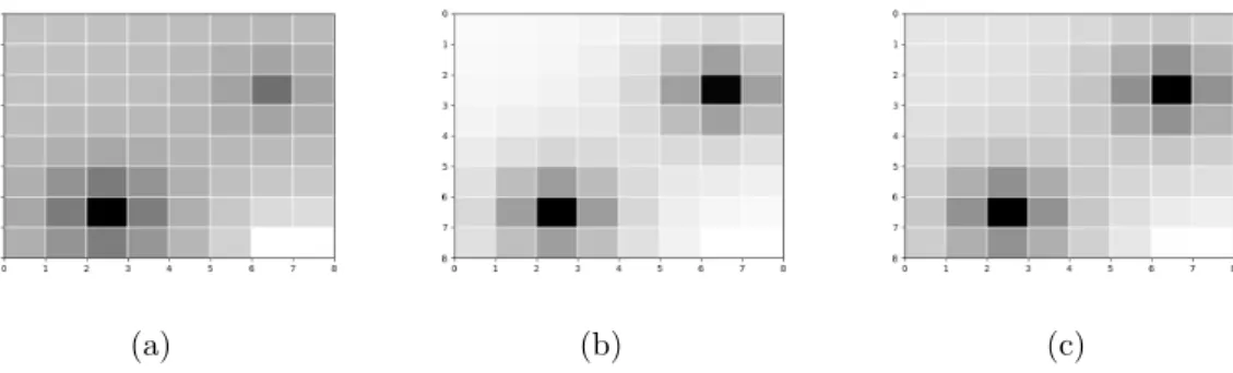
(a) (b) (c)
Figure 4·1: (a)p∗ = 90%. The learnt policy has a probability of 12.5% with respect to the given PCTL property. The reward function assigns lower rewards to the unsafe states than the states nearby. (b)p∗ = 40%. The learnt policy has a probability of 11.0% with respect to the given PCTL property. The reward function assigns even lower rewards to the unsafe states, indicated by the greater contrast between unsafe states and other states. (c)p∗ = 10%. The learnt policy has a probability of 4% with respect to the given PCTL property. The reward function assigns such low rewards to the unsafe states that the states nearby are also assigned with low rewards (because of the radial basis feature functions).
Table 4.1: Average runtime per iteration in seconds.
Size Num. of States Compute π Compute µ MC Cex
8×8 64 0.02 0.02 1.39 0.014
16×16 256 0.05 0.05 1.43 0.014
32×32 1024 0.07 0.08 3.12 0.035
64×64 4096 6.52 25.88 22.877 1.59
using the grid-world example. The first and second columns indicate the size of the grid world and the resulting state space. The third column shows the average run-time that policy iteration takes to compute an optimal policy π for a known reward function. The forth column indicates the average runtime that policy iteration takes to compute the expected features µ for a known policy. The fifth column indicates
the average runtime of verifying the PCTL formula using PRISM. The last column indicates the average runtime that generating a counterexample using COMICS.
4.2
Cart-Pole from OpenAI Gym
(a) (b)
(c)
Figure 4·2: (a) The cartpole environment. (b) The cart is at -0.3 and pole angle is -20◦. (c) The cart is at 0.3 and pole angle is 20◦.
In grid world, it is hard to evaluate the performance that the agent may need to sacrifice for safety. Hence we implement the algorithm in OpenAI gym environments where performance can be quantified. In the cart-pole environment as shown in Fig. 4·2(a), the goal is to keep the pole on a cart from falling over as long as possible by moving the cart either to the left or to the right in each time step. The maximum
step length is t = 200. The position, velocity and angle of the cart and the pole are continuous values and observable, but the actual dynamics of the system are unknown.
We discretize the continuous observation space and formulate the environment as an MDP with 400 states and 2 actions. Through exploring the environment, the transition function is determined by the samples of experienced transitions. The feature vector in each state contains 30 radial basis functions which depend on the squared Euclidean distances between current states and other 30 states which are uniformly distributed in the state space. In addition, a maneuver is deemed unsafeif the pole angle is larger than 20◦ while the cart’s horizontal position is more than±0.3 as shown in Fig. 4·2(b) and 4·2(c). We formalize the safety requirement in PCTL as (4.1).
Φ ::=P≤p∗[true U≤t (angle≤ −20◦ ∧position≤ −0.3)
∨(angle≥20◦ ∧position≥0.3)]
(4.1)
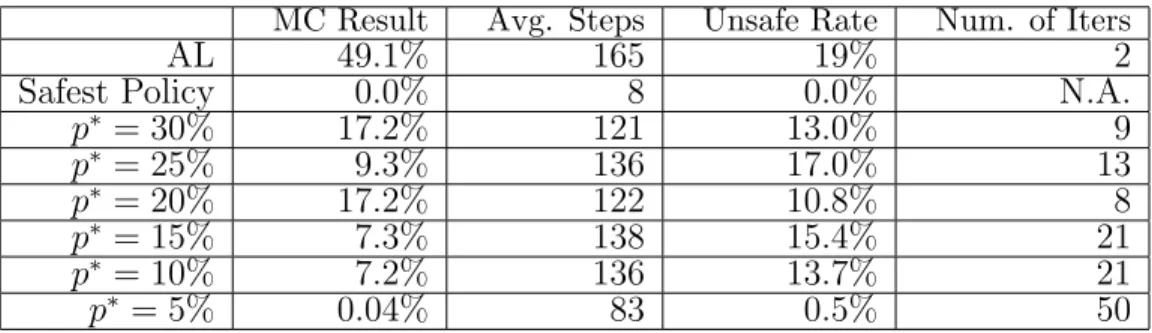
Table 4.2: In the cart-pole environment, higher average steps mean better performance. The safest policy is synthesized using PRISM-games.
MC Result Avg. Steps Unsafe Rate Num. of Iters
AL 49.1% 165 19% 2
Safest Policy 0.0% 8 0.0% N.A.
p∗ = 30% 17.2% 121 13.0% 9 p∗ = 25% 9.3% 136 17.0% 13 p∗ = 20% 17.2% 122 10.8% 8 p∗ = 15% 7.3% 138 15.4% 21 p∗ = 10% 7.2% 136 13.7% 21 p∗ = 5% 0.04% 83 0.5% 50
We consider only demonstrations for which the pole is held upright without vio-lating any of the safety conditions for all 200 steps. The safest policy synthesized by PRISM-games is used as the initial safe policy. We also compare the different policies
learned by CEGAL for different safety threshold p∗s. In Table 4.2, the policies are compared in terms of model checking results (‘MC Result’) on the PCTL property in (4.1) using the constructed MDP, the average steps (‘Avg. Steps’) that a policy (executed in the OpenAI environment) can hold across 5000 rounds (the higher the better), and averaged percentage times (‘Unsafe Rate’) that a policy (executed in the OpenAI environment) violates the unsaf e conditions across 5000 rounds. The last column in the table shows the averaged number of iterations for these algorithms to converge (with 50 as the maximum number of iterations). The policy in the first row is the result of using AL alone. Observe that fromp∗ = 30% to 10%, the performance of the learnt policy is similar. However, when the safety threshold becomes very low, e.g., p∗ = 5%, the performance of the learnt policy drops significantly. Observe also that the safest policy has the lowest performance amongst all. It corresponds to simply letting the pole fall and thus does not risk moving the cart out of the range [-0.3, 0.3]. We note that the discrepancy between the ‘MC result’ and the ‘unsafe rate’ is due to the MDP abstraction of the actual game environment. The safety guarantee of the algorithm is based on the former and the latter is used for validation purposes. The discordances between model checking results and unsafe rates are due to the inaccurate transition function. Despite the inconsistency, the policies learnt via CEGAL still show lower frequency of reaching unsafe states than that via AL.
4.3
Mountain-Car from OpenAI Gym
Our third experiment uses the mountain-car environment from OpenAI Gym. As shown in Fig. 4·3(a), a car starts from the bottom of the valley and tries to reach the mountaintop on the right as quickly as possible. In each time step the car can perform one of the three actions, accelerating to the left, coasting, and accelerating to the right. The agent fails if the step length reaches the maximum (t = 66). The
(a)
(b)
Figure 4·3: (a) The original mountain-car environment. (b) The mountain-car environment with traffic rules: when the distance from the car to the left edge or the right edge is shorter than 0.1, the speed of the car should be lower than 0.04.
velocity and position of the car are continuous values and observable while the exact dynamics are unknown.
We discretize the continuous observation space and formulate the environment as an MDP with 320 states and 3 actions. Through exploring the environment, the transition function is determined by the samples of experienced transitions. The feature vector for each state contains 2 exponential functions and 18 radial basis functions which respectively depend on the squared Euclidean distances between the current state and other 18 states which are uniformly distributed in the state space. In
this game setting, the car cannot reach the right mountaintop by simply accelerating to the right. It has to accumulate momentum first by moving back and forth in the valley. The safety rules we enforce are shown in Fig. 4·3(b). They correspond to speed limits when the car is close to the left mountaintop or to the right mountaintop (in case it is a cliff on the other side of the mountaintop). Similar to the previous experiments, we consider only expert demonstrations that successfully reach the right mountaintop without violating any of the safety conditions. The average step length of demonstrations is 40. We formalize the safety requirement in PCTL as (4.2).
Φ ::=P≤p∗[true U≤t (speed ≤ −0.04∧position≤ −1.1)
∨(speed ≥0.04∧position≥0.5)]
(4.2)
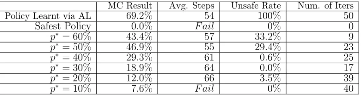
Table 4.3: In the mountain-car environment,loweraverage steps mean better performance. The safest policy is synthesized via PRISM-games.
MC Result Avg. Steps Unsafe Rate Num. of Iters
Policy Learnt via AL 69.2% 54 100% 50
Safest Policy 0.0% F ail 0% 0
p∗ = 60% 43.4% 57 33.2% 9 p∗ = 50% 46.9% 55 29.4% 23 p∗ = 40% 29.3% 61 0.6% 25 p∗ = 30% 18.9% 64 0.0% 17 p∗ = 20% 12.0% 66 3.5% 39 p∗ = 10% 7.6% F ail 0% 40
We compare the different policies using the same set of categories as in the cart-pole example. The numbers are averaged over 5000 rounds. The last column in the table shows the averaged number of iterations for these algorithms to converge (with 50 as the maximum number of iterations). As shown in the first row, the policy learnt via AL has the highest probability of going over the speed limits. We observe that this policy makes the car speed up all the way to the left mountaintop to maximize its potential energy. The safest policy corresponds to simply staying in the bottom of
the valley. The policies learnt via CEGAL for the safety thresholdp∗ranges from 60% to 50% not only have lower probability of violating speed limits but also maintain comparable performance. However, when the safety threshold p∗ further decreases, the agent becomes more conservative and it takes more time for the car to finish the task. The discordances between model checking results and unsafe rates are due to the inaccurate transition function. Despite the inconsistency, the policies learnt via CEGAL still show obvious restraint in reaching unsafe states than that via AL.
4.4
Discussion
In the three experiments, we evaluate our algorithm in different aspects. From the gridworld experiment, we observe how safety specification influences the implicit search for reward function in our algorithm. When the safety threshold decreases, lower rewards will be assigned to the unsafe states so that the optimal policy with respect to the reward function will avoid reaching those states. From cart-pole and mountain-car experiments, we observe how our algorithm guarantees the safety of the final output policy while retaining the performance of the learnt policy in the mean time. In both experiments, by learning from human demonstrations and the counterexamples for violating the safety specification, the agent not only knows how to finish the tasks but also exhibits the awareness of safety.
Chapter 5
Conclusions
5.1
Summary of the thesis
In this thesis, a counterexample-guided approach is proposed for combining formal verification with apprenticeship learning to ensure safety of the learning outcome. By giving a safety specification and adding a verification oracle to the original appren-ticeship learning algorithm, it is guaranteed that only a policy that satisfies the safety specification will be output. Furthermore, when a learnt policy is verified to violate the safety specification, a counterexample, which is a proof of the violation, will be extracted from the policy. Without having to risk deploying the unsafe policy in the field, a counterexample can be regarded as a set of negative examples. The approach in this thesis makes novel use of the counterexamples to steer the policy search pro-cess by formulating the problem as a multi-objective optimization problem. By using an adaptive weight approach, the multi-objective optimization problem is solved it-eratively. The multi-objective weight parameter is updated according to the learnt policy in each iteration. The algorithm is guaranteed to terminate when the multi-objective weight parameter converges to a certain value. The experimental results indicate that the proposed approach can guarantee safety and retain performance for a set of benchmarks including examples drawn from OpenAI Gym.
In addition to what have been achieved in this thesis, there are some open chal-lenges in the theories of the algorithm. Firstly, this thesis does not guarantee finding a safe policy that performs as well as expert policy. Although it is common sense
that being safe can sometimes conflicts with having high performance, finer control in leverage between different objects would be beneficial. More specifically, when solving the multi-objective optimization problem, although an adaptive weight sum approach is employed, the algorithm does not end up with the Pareto frontier. Although the linear constraints ensures the dominance of the optimal π, ˆπ and cex in individual iteration, more candidate policies and counterexamples will be found as the iteration continues. Thus, the dominance in one iteration may not hold in the future iteration. One shortcoming of the thesis is in the termination of the algorithm which is fully based on the multi-objective parameter rather than converging to the global optimum of the solved policy. There are also challenges in model construction which brings the gap between the margin of policy features and margin of the true policy performance. In OpenAI gym environments, where performance can be quantified, a learnt policy that is -close to the expert policy does not necessarily have performance quantita-tively comparable with expert policy. Whereas, this requires dedicated feature design for the reward function as well as more accurate transition function, which is out of the scope of this thesis.
5.2
Future Work
In the future, firstly we plan to deploy our framework in tasks more complex than the OpenAI gym environments, such as ROS1 environment and Baxter2 robot.
Secondly, we will test the scalability of the current verification techniques uti-lized in our prototype. Different methods in policy verification and counterexample generation will also be considered in case of necessity of improving the efficiency of the framework. For instance, we are considering applying statistical model check-ing (Younes et al., 2011), (Younes and Simmons, 2006), (Henriques et al., 2012) in
1
http://wiki.ros.org/ROS/Tutorials/InstallingandConfiguringROSEnvironment 2
large scale learning tasks where the state space may be too large for symbolic model checking techniques.
In addition, we will concentrate on addressing the theoretical shortcomings in the CEGAL algorithm. For instance, we will consider using gradient based method as in (Neu and Szepesv´ari, 2012), rather than iteration based method, to solve appren-ticeship learning problem or other imitation learning problems, such as the model-free method in (Ho et al., 2016). Meanwhile, we will investigate new ways to incorporate counterexample in the learning process.
Abbeel, P. and Ng, A. Y. (2004). Apprenticeship learning via inverse reinforcement learning. In Proceedings of the Twenty-first International Conference on Machine Learning, ICML ’04, pages 1–, New York, NY, USA. ACM.
Abrah´am, E., Jansen, N., Wimmer, R., Katoen, J.-P., and Becker, B. (2010). Dtmc model checking by scc reduction. In2010 Seventh International Conference on the Quantitative Evaluation of Systems (QEST), pages 37–46. IEEE.
Alshiekh, M., Bloem, R., Ehlers, R., K¨onighofer, B., Niekum, S., and Topcu, U. (2017). Safe reinforcement learning via shielding. CoRR, abs/1708.08611.
Amodei, D., Olah, C., Steinhardt, J., Christiano, P., Schulman, J., and Man´e, D. (2016). Concrete problems in AI safety. CoRR, abs/1606.06565.
Bellman, R. (1957). A markovian decision process. Journal of Mathematics and Mechanics, pages 679–684.
Bundy, A. (2016). Preparing for the future of artificial intelligence.
Fujita, M., McGeer, P. C., and Yang, J.-Y. (1997). Multi-terminal binary decision diagrams: An efficient data structure for matrix representation. Formal methods in system design, 10(2-3):149–169.
Gillulay, J. H. and Tomlin, C. J. (2011). Guaranteed safe online learning of a bounded system. In 2011 IEEE/RSJ International Conference on Intelligent Robots and Systems (IROS), pages 2979–2984. IEEE.
Han, T., Katoen, J. P., and Berteun, D. (2009). Counterexample generation in prob-abilistic model checking. IEEE Transactions on Software Engineering, 35(2):241– 257.
Hansson, H. and Jonsson, B. (1994). A logic for reasoning about time and reliability.
Formal Aspects of Computing, 6(5):512–535.
Held, D., McCarthy, Z., Zhang, M., Shentu, F., and Abbeel, P. (2017). Probabilisti-cally safe policy transfer. CoRR, abs/1705.05394.
Henriques, D., Martins, J. G., Zuliani, P., Platzer, A., and Clarke, E. M. (2012). Sta-tistical model checking for markov decision processes. In2012 Ninth International Conference on Quantitative Evaluation of Systems (QEST), pages 84–93. IEEE.
Ho, J., Gupta, J., and Ermon, S. (2016). Model-free imitation learning with policy optimization. InInternational Conference on Machine Learning, pages 2760–2769. Jansen, N., ´Abrah´am, E., Scheffler, M., Volk, M., Vorpahl, A., Wimmer, R., Katoen, J., and Becker, B. (2012). The COMICS tool - computing minimal counterexam-ples for discrete-time markov chains. CoRR, abs/1206.0603.
Jha, S. and Seshia, S. A. (2017). A theory of formal synthesis via inductive learning.
Acta Informatica, 54(7):693–726.
Junges, S., Jansen, N., Dehnert, C., Topcu, U., and Katoen, J.-P. (2016). Safety-constrained reinforcement learning for mdps. In International Conference on Tools and Algorithms for the Construction and Analysis of Systems, pages 130– 146. Springer.
Krizhevsky, A., Sutskever, I., and Hinton, G. E. (2012). Imagenet classification with deep convolutional neural networks. InAdvances in neural information processing systems, pages 1097–1105.
Kuo, Y.-J. and Mittelmann, H. D. (2004). Interior point methods for second-order cone programming and or applications. Computational Optimization and Applica-tions, 28(3):255–285.
Kwiatkowska, M., Norman, G., and Parker, D. (2002). Prism: Probabilistic symbolic model checker. Computer Performance Evaluation/TOOLS, 2324:200–204.
Kwiatkowska, M. and Parker, D. (2013). Automated Verification and Strategy Syn-thesis for Probabilistic Systems, pages 5–22. Springer International Publishing, Cham.
Kwiatkowska, M., Parker, D., and Wiltsche, C. (2017). Prism-games: verification and strategy synthesis for stochastic multi-player games with multiple objectives.
International Journal on Software Tools for Technology Transfer.
Levinson, J., Askeland, J., Becker, J., Dolson, J., Held, D., Kammel, S., Kolter, J. Z., Langer, D., Pink, O., Pratt, V., et al. (2011). Towards fully autonomous driving: Systems and algorithms. In2011 IEEE Intelligent Vehicles Symposium (IV), pages 163–168. IEEE.
Mason, G. R., Calinescu, R. C., Kudenko, D., and Banks, A. (2017). Assured reinforcement learning for safety-critical applications. In Doctoral Consortium at the 10th International Conference on Agents and Artificial Intelligence. SciTePress. Mnih, V., Kavukcuoglu, K., Silver, D., Rusu, A. A., Veness, J., Bellemare, M. G., Graves, A., Riedmiller, M., Fidjeland, A. K., Ostrovski, G., et al. (2015). Human-level control through deep reinforcement learning. Nature, 518(7540):529–533.
Moldovan, T. M. and Abbeel, P. (2012). Safe exploration in markov decision pro-cesses. arXiv preprint arXiv:1205.4810.
Neu, G. and Szepesv´ari, C. (2012). Apprenticeship learning using inverse reinforce-ment learning and gradient methods. arXiv preprint arXiv:1206.5264.
Ng, A. Y. and Russell, S. J. (2000). Algorithms for inverse reinforcement learning. In Proceedings of the Seventeenth International Conference on Machine Learning, ICML ’00, pages 663–670, San Francisco, CA, USA. Morgan Kaufmann Publishers Inc.
Puggelli, A., Li, W., Sangiovanni-Vincentelli, A. L., and Seshia, S. A. (2013). Polynomial-time verification of pctl properties of mdps with convex uncertainties. In Proceed-ings of the 25th International Conference on Computer Aided Verification, CAV’13, pages 527–542, Berlin, Heidelberg. Springer-Verlag.
Ratliff, N. D., Bagnell, J. A., and Zinkevich, M. A. (2006). Maximum margin plan-ning. In Proceedings of the 23rd International Conference on Machine Learning, ICML ’06, pages 729–736, New York, NY, USA. ACM.
Sadigh, D., Kim, E. S., Coogan, S., Sastry, S. S., and Seshia, S. A. (2014). A learning based approach to control synthesis of markov decision processes for linear temporal logic specifications. In2014 IEEE 53rd Annual Conference on Decision and Control (CDC), pages 1091–1096. IEEE.
Shiarlis, K., Messias, J., and Whiteson, S. (2016). Inverse reinforcement learning from failure. InProceedings of the 2016 International Conference on Autonomous Agents & Multiagent Systems, pages 1060–1068. International Foundation for Autonomous Agents and Multiagent Systems.
Solar-Lezama, A., Tancau, L., Bodik, R., Seshia, S., and Saraswat, V. (2006). Com-binatorial sketching for finite programs. pages 404–415.
Wimmer, R., Jansen, N., ´Abrah´am, E., Becker, B., and Katoen, J.-P. (2012). Mini-mal Critical Subsystems for Discrete-Time Markov Models, pages 299–314. Springer Berlin Heidelberg, Berlin, Heidelberg.
Younes, H. L. S., Clarke, E. M., and Zuliani, P. (2011). Statistical verification of probabilistic properties with unbounded until. In Davies, J., Silva, L., and Simao, A., editors,Formal Methods: Foundations and Applications, pages 144–160, Berlin, Heidelberg. Springer Berlin Heidelberg.
Younes, H. L. S. and Simmons, R. G. (2006). Statistical probabilistic model checking with a focus on time-bounded properties. Inf. Comput., 204(9):1368–1409.
Ziebart, B. D., Maas, A., Bagnell, J. A., and Dey, A. K. (2008). Maximum entropy inverse reinforcement learning. In Proceedings of the 23rd National Conference on Artificial Intelligence - Volume 3, AAAI’08, pages 1433–1438. AAAI Press.