Assessing the Effect of Visualizations on Bayesian Reasoning through Crowdsourcing

Assessing the Effect of Visualizations on Bayesian Reasoning

through Crowdsourcing

Luana Micallef, Pierre Dragicevic, and Jean-Daniel Fekete,Member, IEEE

Fig. 1. The six visualizations evaluated in our study, illustrating the classic mammography problem [21].

Abstract—People have difficulty understanding statistical information and are unaware of their wrong judgments, particularly in Bayesian reasoning. Psychology studies suggest that the way Bayesian problems are represented can impact comprehension, but few visual designs have been evaluated and only populations with a specific background have been involved. In this study, a textual and six visual representations for three classic problems were compared using a diverse subject pool through crowdsourcing. Visualizations included area-proportional Euler diagrams, glyph representations, and hybrid diagrams combining both. Our study failed to replicate previous findings in that subjects’ accuracy was remarkably lower and visualizations exhibited no measurable benefit. A second experiment confirmed that simply adding a visualization to a textual Bayesian problem is of little help, even when the text refers to the visualization, but suggests that visualizations are more effective when the text is given without numerical values. We discuss our findings and the need for more such experiments to be carried out on heterogeneous populations of non-experts. Index Terms—Bayesian reasoning, base rate fallacy, probabilistic judgment, Euler diagrams, glyphs, crowdsourcing.

1 INTRODUCTION

Both laymen and professionals have difficulty making inferences and decisions based on statistical and probabilistic data [18, 26, 32]. This can have severe consequences in many domains.

Physicians need to diagnose diseases based on the outcome of reliable medical tests. Patients need to decide whether they should un-dertake heavy medical treatment. Wrong judgments are common and

• Luana Micallef is with INRIA and School of Computing, University of Kent, UK, e-mail: [email protected].

• Pierre Dragicevic is with INRIA, e-mail: [email protected].

• Jean-Daniel Fekete is with INRIA, e-mail: [email protected]. Manuscript received 31 March 2012; accepted 1 August 2012; posted online 14 October 2012; mailed on 5 October 2012.

For information on obtaining reprints of this article, please send e-mail to: [email protected].

often result in overdiagnosis [55], e.g., up to two thirds of breast can-cers detected by mammography can be overdiagnosed [58]. In other cases, patients with a positive HIV test result attempted or committed suicide before further tests turned out negative [13, 25, 50]. In this domain, a crucial piece of information for effective decision making is the probability that a patient has a disease given that a test is positive.

In legal trials, juries have to convict or acquit defendents based on unreliable evidence and here too, wrong judgments abound [36]. A respected professor and advisor to defense lawyers claimed on U.S. television that since only 0.1% of wife batterers murder their wives, evidence of battering should be ignored in murder trials [29]. This reasoning is however fallacious, since the only important information is the probability that a husband was the murderer given that he bat-tered his wife and she was killed.

These two scenarios involve Bayesian inference, which is known to be counterintuitive and subject to fallacious reasoning. As an illustra-tion, consider the following classic problem [21]:

The probability that a woman at age 40 has breast cancer is 1%. According to the literature, the probability that the disease is detected by a mammography is 80%. The prob-ability that the test misdetects the disease although the pa-tient does not have it is 9.6%.

If a woman at age 40 is tested as positive, what is the prob-ability that she indeed has breast cancer?

Out of 100 doctors, 95 estimated this probability to be between 70% and 80%, while the correct probability is only 7.8% [21]. The prob-ability is low because the prevalence of the disease in the population, i.e., thebase rate, is low. When making Baysian inference, this infor-mation is often ignored [27, 32], thus leading to the base rate fallacy [4, 5]. Using natural frequencies1instead of probabilities reduces the fallacy [18, 27, 31]. However, it is still difficult to comprehend how the different numerical quantities relate to each other2.

Previously proposed solutions involve the use of heuristics [34] and theories of mental models [33]. Others use visual representations. A study confirms that when Bayes’ theorem is introduced to students through visualizations, students learn faster and report higher tempo-ral stability than without a visualization [48]. However, prior training is not always possible. A few studies were conducted to assess the immediate benefits of visualizations, but it is still unclear which is the most effective representation for Bayesian reasoning. Moreover, stud-ies have been carried out on populations with a specific background (usually highly-focused university students), making it difficult to gen-eralize their findings to a more diverse population of laypeople of var-ious backgrounds and ages.

We present the first study that tests the effectiveness of six different visualizations (i.e., Euler diagrams, glyph representations, and combi-nations of the two) on a large, diverse group of participants through crowdsourcing. Two new textual problem formats, specially designed to be used with visualizations, are also proposed and evaluated.

We first discuss current visualizations for Bayesian reasoning (Sec-tion 2). Then, we introduce the ra(Sec-tionale of our study design (Sec(Sec-tion 3) and we report our two experiments together with our findings and their implications (Sections 4 and 5). Finally, we summarize our work and contributions (Section 6).

2 VISUALIZATIONS FORBAYESIANREASONING

Several visual representations have been considered for Bayesian problems, including trees [48], “beam cut” pictorial analogs [27], con-tingency tables [15, 16], signal detection curves [15, 16], detection bars [15, 16], Bayesian boxes [10], and bar-grain boxes [10]. Some of them, such as signal detection curves, are difficult to understand and require subject training prior to the experiment [15, 16].

Two straightforward and popular visualizations in research are Eu-ler diagramsandfrequency grids. Studies suggest that Euler diagrams can clarify thenested-set relations(i.e., how the different pieces of nu-merical data relate) of Bayesian problems [49], while frequency grids are believed to facilitate logical reasoning [8, 18]. Our work focuses on these two types of visualizations and combinations of both.

2.1 Euler Diagrams

Sloman et al. [49] argued that Euler diagrams as in Figure 1-V1 are effective in conveying the nested-set relations of Bayesian problems (48% out of 25 participants gave a correct answer with Euler diagrams and text vs. 20% out of 25 with text alone - both using probabilities). However, expliciting nested-set relations in the text yielded similar benefits. Later, Brase [8] found no improvement with Euler diagrams (34.7% success out of 98 with Euler diagrams, 35.4% out of 96 with text alone - both using natural frequencies). Yet, Euler diagrams have been shown to clarify nested-set relations in problems involving in-ductive [57] and dein-ductive [6] reasoning.

1_{Usingnatural frequencieswould mean stating “10 out of every 1,000}

women” instead of giving a 1% probability. This frequency format is said to be naturalas the denominator corresponds to the number of actual observations.

2_{In our example, 1% is thebase rate, 80% is thehit rate, and 9.6% is the}

false alarm rate.

Studies in psychology tend to ignore Euler diagram design issues. For example, in both Sloman et al.’s and Brase’s studies, Euler dia-grams were not exactly area-proportional, meaning that the area of the regions was not proportional to the quantities they were meant to visualize and, this could have possibly made the diagrams misleading. In contrast, Euler diagram design has been discussed extensively in computer science and, various automatic generation algorithms have been developed (e.g., [17, 38, 43, 44, 56]). However, apart from a few exceptions [7, 43, 45], few user studies have been conducted in com-puter science and, none of them focused on a particular application area, such as Bayesian problem solving. As far as we know, our work is the first at the intersection of the two disciplines.

2.2 Frequency Grids

Cosmides and Tooby [18] argued that representations with discrete, countable objects like frequency grids, as in Figure 1-V3, facilitate logical reasoning, but found no improvement over text alone (76% success among 75 participants with frequency grid, 76% out of 50 with text alone using natural frequencies). They believed that visu-alizations were ignored and found that guiding subjects into actively drawing their own frequency grids resulted in a notably improved suc-cess rate of 92% out of 25. Similarly, after training, Sedlmeier and Gigerenzer [48] observed a success rate of 75% then 100% five weeks later among 14 subjects who drew frequency grids, compared to 60% then 20% (as before training) in 20 subjects applying Bayes’ theorem. Yet, later, Brase [8] reported no improvement between passive and actively drawn grids (49% out of 49 for active, 48.4% out of 95 for passive). Cole and Davidson [16] agree that subjects become highly accurate and fast when trained in using frequency grids compared to text alone, but found no significant difference in errors between fre-quency grids and other visualizations.

Studies in frequency grid design for risk communication suggest that visualizations made up of two grids are perceived faster [42] and those showing just the section of interest facilitate reasoning for low probabilities [20]. For Bayesian reasoning, Brase [8] compared fre-quency grids with regular and random layouts, but found no difference in success rate (47.6% out of 42 subjects for both).

2.3 Hybrid Diagrams

Euler diagrams can convey critical information on the nested-set rela-tions of Bayesian problems [28, 49], while representarela-tions with dis-crete objects (e.g., glyphs) can facilitate logical reasoning [18]. Thus, combining the two approaches by embedding glyphs in Euler dia-grams, as in Figure 1-V4, V5 and V6, would seem beneficial.

We only know of one study, that by Brase [8], which evaluated hy-brid diagrams as in Figure 1-V4 but using an Euler diagram as in Fig-ure 1-V1. Results suggest that such diagrams do not increase success rates compared to standard Euler diagrams or frequency grids (41.7% out of 108 for hybrid, 48.4% out of 95 for frequency grid, 34.7% out of 98 for Euler diagram, 35.4% out of 96 for text alone). Also, when subjects were instructed to draw their visualization as in [18], hybrid diagrams were even less effective (28% out of 50 for hybrid, 49% out of 49 for frequency grid, 30% out of 50 for Euler diagram).

However, the visualization designs used in Brase’s study have a number of issues:i)the hybrid diagram was area-proportional whereas the pure Euler diagram was not, introducing a possibility of experi-mental confound;ii)the number of glyphs in the hybrid diagram was inconsistent with the numerical data (in the experiment comparing the hybrid with the standard frequency diagram);iii)the hybrid diagram and the frequency diagram used different glyph shapes (dots vs. an-thropomorphic), introducing another possibility of confound.

In addition, like most other studies, Brase’s study involved a pop-ulation of university students who had to participate in the study as part of their psychology course requirement. Also, only one medical diagnosis problem was evaluated, making it difficult to generalize the findings to other problems. In the following section, we explain how we address most of these limitations.

3 STUDYDESIGNRATIONALE

In this section, we motivate and justify our study design, including the use of crowdsourcing, our different visualization designs, our choices of Bayesian problems, and our performance measures.

3.1 Crowdsourcing

As mentioned before, most studies on Bayesian reasoning employed populations with a specific background, often students [8, 27, 49], which poses problems in terms of generalizability. For example, stu-dents are typically 20 years old, while human capabilities to process information decline with age, with the best performance being in early twenties [47]. Another issue is ecological validity, since probabilistic reasoning in the real world is different from a university setting where students are trained to remain focused and make the best use of their cognitive resources in order to solve a problem given by a professor.

For these reasons, we considered crowdsourcing and we used MTurk [12, 40] as a technology to automatically outsource simple tasks to a network of Internet users. The tasks posted byrequestersare calledHITs(Human Intelligence Tasks) and are completed by anony-mousworkerswho get a monetary reward, if successful. Although crowdsourcing platforms have not been initially designed for conduct-ing experiments, their use in research became popular [12], includconduct-ing in information visualization [30]. The demographics of workers is now well-understood [46] and a methodology is being developed for designing effective experiments and addressing concerns such as sci-entific control [30, 40].

Although crowdsourced experiments are subject to many of the same problems as laboratory experiments, they capture some inter-esting aspects of real-world problem solving. First, they capture a large and diverse population with different backgrounds, levels of ed-ucation and occupations, age groups and gender [46]. Furthermore, workers typically try to complete as many HITs as possible (most of-ten for personal satisfaction), while a rating system provides them with incentives for being accurate [40]. Since workers typically complete several HITs in sequence, they cannot focus on a single task as much as participants to a laboratory experiment. We believe this better cap-tures many situations when decisions have to be made accurately and rapidly. In addition, due to the informal setup, workers might be less subject to experimental biases such as demand characteristics [39].

Finally, setting up an experiment on a crowdsourcing platform can be initially costly, but the time and effort for running subjects is much lower than in laboratory experiments. With the notable exception of Brase’s study [8] that involved 412 undergraduates students, previous studies on Bayesian reasoning typically involved about 50 participants [27, 49]. Therefore, small effects cannot be detected and results have been rarely reported on two conditions being similar. Crowdsourcing gives access to more statistical power and makes it easier to test mul-tiple, diverse hypotheses such as those involving equivalence.

3.2 Visualization Designs

Previous studies examined whether visualizations can facilitate Bayesian reasoning, but only one or a few visualizations were com-pared at a time. In addition, the choices made in terms of visualiza-tion design were rarely discussed and often inconsistent. Overall, this makes it hard to interpret and compare findings across studies.

To address this, we propose a set of visualization designs (V1-V6) that involve Euler-based representations, glyph-based represen-tations, and combinations of the two. Consistent with the tradition of HCI and infovis research, our goal is to start paving the design space based on clear design rationales, while keeping unimportant de-sign details as consistent as possible in order to better tease out the effects of important design features. Novel algorithms (not discussed in this article) were developed to automatically generate all of these visualizations for any Bayesian problem. The software is available at

http://www.eulerdiagrams.org/eulerGlyphs. Figure 1 shows the visualizations generated for the classic mammography prob-lem [21].

In the following sections,area-proportionalwill be denoted as AP.

V1: AP Euler Diagram with a 1-Set Population

Similar to the Euler diagrams proposed by Brase [8] and Sloman et al. [49], the entire population in V1 is represented as one set that is shown as a green circle in Figure 1-V1. The interior of the black circle is divided in two: the red area corresponds to the hit rate, while the remaining area corresponds to the false alarm rate. All the curves and the intersecting regions are exactly area-proportional to the values in the problem. Thus, the ratio between the hit rate area and the black circle area is the answer to the Bayesian problem.

V1 is the only diagram representing the entire population and thus, its design unavoidably differs in several respects. The other diagrams represent the entire population as two regions shaded in red and blue. To reduce the differences, we initially shaded the region inside the en-tire population circle and outside the red circle of V1 in blue. However, an early pilot study revealed that this could be misleading as subjects assumed that the red circle formed part of the blue region (the blue re-gion is the entire population minus the red circle). After trying several unsuccessful variants, we opted to display the entire population circle as an outline in a color different from red and blue, thus green. V2: AP Euler Diagram with a 2-Set Population

V2 is a variant of V1 initially proposed (but not evaluated) by Kellen et al. [35], where the entire population is split up into two sets (the red and blue circles in Figure 1-V2). The complementarity of the two pop-ulation sets is enhanced using disjoint circles and contrasting colors. Since the third set represents a different concept, a different shape (an ellipse) is used and only its outline is displayed. This makes the third set distinguishable from the other two population sets, consistent with the Gestalt principle of good continuation [37] and thus, easy to per-ceive. We anticipated that compared to V1, this design would clarify the nested-set relationships and facilitate Bayesian reasoning.

The regions in V2 are exactly area-proportional to the values in the problem with the exception of two white regions which, as illustrated in Figure 1, are irrelevant to the problem. These extra regions can be eliminated by replacing the two population circles with rectangles. However, the diagram would be less familiar to users and likely more difficult to read due to a lack of good continuation. As shown in V4, V5 and V6, this issue is mitigated by having all regions white and overlaid by a number of colored glyphs representing the region’s value. Regions with no glyphs look empty and irrelevant to the problem. V3: Frequency Grid

V3 maps circular glyphs to different sets in the Bayesian problem, with as many glyphs as members of the population. The design is rep-resentative of typical designs in the literature on risk communication, including the horizontal ruler provided to facilitate cardinality estima-tion. The same color coding scheme (solid and outline colors) as V2 is used to convey set membership of glyphs.

Glyphs of different shapes have been used before, including simple geometrical shapes [24] and icons such as anthropomorphic figures [2, 8, 9]. Although icons are often thought to provide benefits, a study reports no significant improvement over simple shapes for such visu-alizations [51]. In addition, icons are problem-dependent (not all pop-ulations represent people) and can make diagrams cluttered and hard to read [24, 51]. Therefore, we opted for circles. Studies on hybrid visualizations have also employed circles or squares so far [8, 35].

Different layouts have been proposed in the literature. Sometimes, glyphs are laid out horizontally [9], vertically [42] or randomly [8]. A study [42] suggests that horizontal grids are perceived faster. Brase [8] argues that sequential and random placement are both effective, but others [2] suggest that randomness increases subject’s uncertainty as proportions in the diagram are harder to estimate, differences are less intuitive, and larger proportions are perceptually overestimated. We therefore used a sequential layout, but placed glyphs vertically using an ordering for the sets that matches the layout of the regions in V2.

For the grid dimensions, we used aspect ratios that are typical in the literature: a 25×40 grid (for problems with a population of 1000) and a 10×10 grid (for problems with a population of 100). Since glyphs are difficult to label in-place, a separate legend was provided.

V4: AP Euler Diagram + Randomly Positioned Glyphs

V4 consists of the area-proportional Euler diagram V2 with glyphs embedded in corresponding regions using an iterative random place-ment algorithm without packing. It is similar to the visualization stud-ied in [8] except that the Euler diagram is exactly area-proportional and the numbers of glyphs match the values in the problem. Thus, glyph density is constant across regions. For this design, as well as hybrids V5 and V6, the size and shape of the glyphs is consistent with V3 but due to their layout, no ruler can be shown. Both a legend (for glyphs) and in-place labels (for Euler curves) are provided.

V5: Not AP Euler Diagram + Uniformly Positioned Glyphs This hybrid visualization is similar to V4 but employs a regular grid layout with the same glyph spacing as in V3. Automatically drawing these diagrams is more difficult than with other hybrids, as the small-est curves that enclose the glyphs have to be drawn after glyphs are positioned in the correct regions. Thus, the Euler diagram is more compact but not proportional, although it is often close to area-proportional especially for regions with many glyphs.

V6: Not AP Euler Diagram + Frequency Grid Glyphs

Whereas V4 and V5 can be seen as “Euler-oriented” hybrid diagrams where glyphs appear to have been added to the regions of an Euler dia-gram (V2), V6 is a “Frequency grid - oriented” hybrid diadia-gram where Euler curves appear to have been added to a frequency grid (V3). No attempt was made to ensure the Euler curves are area-proportional. Brases’s study [8] involves a similar representation, but uses rectangu-lar Euler curves producing more compact diagrams with greater em-phasis on the frequency grid representation.

3.3 Bayesian Problems

Most previous studies involved a unique Bayesian problem. This could be problematic due to the diverse interests, background, and experi-ence of participants [9, 19]. Studying more than one problem can help level out possible adherence and attachment effects and facilitate the generalization of the experiment findings. A classic study [27] evalu-ated 15 problems, each involving a different scenario. Crowdsourcing experiments have to be short and thus, we chose three problems.

We wanted problems that have been tested in previous studies, are diverse in terms of scenario, and whose base rate, hit rate and false alarm rate are different enough. We opted for a natural frequency for-mat, since it has been shown to work better than probabilities [27, 32]. For these reasons, we chose the following problems (see Table 1): the mammography problem[21],Mam; thecabproblem [3],Cab; and the choosing a course in economicsproblem [1],Eco.

3.4 Measures of Performance

Although most previous studies focus on maximizing and reporting the proportion of correct answers, this dichotomous approach has some limits. First, a percentage of exact answers (say, 75%) says nothing about how far off the remaining 25% are. Second, it is rare that the outcome of a decision depends on a probability estimation being per-fectly exact or not (e.g., making an estimation of 0.001 instead of the correct 0.0012), whereas an estimate of 0.4 versus 0.001 will often produce radically different outcomes. Finally, helping people com-pute an exact answer might be useful in some situations (e.g., teaching probabilities), but is of limited relevance to many real-life situations where one has to make quick decisions and rarely has enough time and attentional resources to sit down and grab a pen or a calculator.

We therefore chose to focus on accuracy, i.e., how far subjects are from the actual answers. Since in the natural frequency format an-swers are provided as a nominator and a denominator (i.e.,v1out of

v2), we start by computing the probabilityp=v1/v2. We believe this

is acceptable since ultimately, the answer is a probability (e.g., the chances of having a cancer). We then compute a bias, which gives the error together with the direction of the error. Although one could use p−pe, with pebeing the exact answer, subtracting probabilities can lead to paradoxes. For example, ifpe=0.01, thenp=0.0000001 would be a more correct answer thanp=0.02. So we uselog10(p/pe)

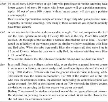
Table 1. The text for the three problems in experiment 1. Mam 10 out of every 1,000 women at age forty who participate in routine screening have

breast cancer. 8 of every 10 women with breast cancer will get a positive mammog-raphy. 95 out of every 990 women without breast cancer will also get a positive mammography.

Here is a new representative sample of women at age forty who got a positive mam-mography in routine screening. How many of these women do you expect to actually have breast cancer?

Cab A cab was involved in a hit-and-run accident at night. Two cab companies, the Red and the Blue, operate in the city. Of every 100 cabs in the city, 15 are Blue and 85 are Red. On the night of the accident, a witness identified the cab as Blue. The court tested the reliability of the witness under the similar visibility conditions with Blue and Red cabs. When the cabs were really Blue, the witness said they were Blue in 12 out of 15 tests. When the cabs were really Red, the witness said they were Blue in 17 out of 85 tests.

What are the chances that the cab involved in the hit-and-run accident was Blue? Eco In a small liberal arts college students take, as an elective, a general interest course

in economics or history. A recent analysis of enrollment figures showed that out of every 1,000 students, 700 students took the general interest course in history, while 300 students took the course in economics. For 210 of the students out of the 300 who took the economics course, the decision on pursuing the economics course was career oriented. For 350 of the students out of the 700 who took the history course, the decision on pursuing the history course was career oriented.

Barbara T. was one of the students who took one of the two general interest courses. Her decision on pursuing the course was career oriented. What are the chances that she had taken the economics course?

instead. The log makes it easy to report and compare large estimation errors. Thus, ifpe=0.01 andp=0.001, then the bias will be−1 and ifp=0.1 the bias will be 1.

We derive theerrorfrom the bias by computing its absolute value. This assumes that a negative bias is as serious as a positive bias, which is a reasonable assumption for problem-independent studies such as our user study. Alternatively, this measure can be adapted to situa-tions where an overestimation is more costly than an underestimation or vice-versa, by pre-multiplying positive or negative biases with a constant. To be able to compare our data with previous experiments, we still report the occurrence of answers for whicherror=0.

In addition to bias and error, we decided to measure the subjects confidence in their answers. This is important because if a visualiza-tion makes people very accurate but not confident at all, then it is of limited use. Conversely, a visualization that makes people very con-fident but plain wrong is harmful, more so than a visualization that makes people less accurate but not overconfident.

Finally, we also decided to measure the time spent reading problems and proving an answer. If workers devote very little time to problems compared to, e.g., laboratory experiment participants, then it could mean that they are not carrying out the task seriously enough. Con-versely, if they devote too much time, then maybe crowdsourcing does not capture quick real-world decision making situations at all.

3.5 Measures of Abilities

A certain level of numeracy ability is required for the understanding and manipulation of natural frequencies [11] and other statistical in-formation [9], while spatial abilities help to efficiently search and re-trieve information. In addition, visualizations might not be helpful to everyone due to different abilities [24] and, the most appropriate vi-sualization could also depend on abilities. For example, Kellen et al. [35] hypothesized that Euler diagrams can facilitate Bayesian reason-ing for those with high spatial abilities, while frequency grids can aid those with high numeracy.

Considering the diversity of MTurk workers, we decided to measure the numeracy and spatial abilities of our participants. Numeracy was measured using the 6-question objective numeracy test from Brown et al. [9] due to the similarities of the subjects’ demographics and their considerations that online subjects are highly educated. To this, we added part 2 of the Subjective Numeracy Scale (SNS) [23]. Spatial abilities were measured using part 1 of the Paper Folding Test (VZ-2) [22]. These are all paper-based tests that we faithfully reimplemented in HTML and JavaScript, including the 3-minute limit for VZ-2.

4 EXPERIMENT1: COMPARISON OFVISUALIZATIONS

The purpose of this first experiment was to test the six different vi-sualizations discussed in Section 3.2 and compare them with text alone. We hypothesized that our visualizations will help subjects solve Bayesian problems. Most of our visualizations were based on a less common Euler diagram representation for Bayesian problems because we anticipated that, by representing the population as two disjoint sets, the reader will be less likely to disregard the base rate. Following pre-vious theories [35], we also hypothesized that subjects with low spatial abilities would benefit from visualizations having discrete and count-able objects, while those with high spatial abilities will benefit mostly from spatial representations such as Euler diagrams.

4.1 Design

As experimental conditions, we had three Bayesian problems and seven visualization types including text alone (V0) and the visualiza-tions in Section 3.2 (V1-V6). Thus, our independent variables were:

• Bayesian problem: PROBLEM∈{Mam,Cab,Eco}; • Visualization type: VIS∈{V0, V1, V2, V3, V4, V5, V6}. Our dependent variables were:

• BIAS, the difference between the subject’s answer and the exact answer, computed as a log ratio;

• ERROR, the absolute value of BIAS; • EX∈ {0,1}, whether the answer is exact; • TIME, the time taken to solve the problem;

• CONF∈[1. .5], the subject’s confidence in his/her answer. Our covariates were:

• NUM∈[0. .30], the subject’s score in the numeracy test; • SPAT∈[0. .10], the subject’s score in the paper folding task. We used a mixed-design approach where each participant was pre-sented the three problems, each accompanied by the same tion type. The use of a between-subjects design for the visualiza-tion factor is consistent with previous studies [8, 18, 49] and prevents asymmetric skill transfer effects [41]. To counterbalance any possi-ble learning effect across propossi-blems, all the six possipossi-ble orderings of the three problems were used. We had 24 participants per visualiza-tion and thus, each of the six problem orderings had one of the seven visualization types and was carried out by four different participants.

4.2 Participants

The participants consisted of 168 crowdsource workers from MTurk. At the end of the HIT, they were asked demographics questions whose answers are summarized in Table 2. These demographics are not fully consistent with some other previous studies on MTurk workers. For instance, the majority of our workers were males (59% in our exper-iment vs. 25% [40] and 48% [46] in MTurk workers studies). Also, considering education and occupation in Table 2, our participants were considerably educated. This could be due to a self-selection bias (re-fer to the HIT title and details in the next section). Five (3%) reported having color blindness, but all of our visualizations used a color-blind friendly palette from ColorBrewer (http://colorbrewer.org).

4.3 Procedure

We first conducted a pilot study with subjects in France and UK (N=14, 2 per visualization type) by hosting the experiment form on a private web page. For the final experiment, HITs were uploaded on MTurk. Once all the required HITs were completed, the workers were granted a qualification to carry out a follow-up questionnaire.

4.3.1 Task

Participants had to fill a form out in their own Web browser. The form was split up into 10 pages and took around 25 minutes to complete. Participants could not review previous pages and could not proceed to the next page without completing all the questions. The first page instructed them to remain focused and not to stop unless all the pages

Table 2. The demographics of the 168 participants.

Gender Female: 41%, Male: 59%

Age Median: 29, Mean: 32, Range:[18,64]

Residence USA: 47%, India: 40%, Other: 13%

Education Bachelor’s Degree: 45%, Some College, No Degree: 22%, Master’s Degree: 15%, Other: 18%

Occupation Professionals, Managers: 38%, Labourers, Service: 30%, Students: 18%, Unemployed, Retired, House-Makers: 15% Color-blind None: 163, Red-green: 4, Other: 1

Percentages may not add up to 100 due to rounding

were completed. The three problems were then presented on separate pages either using text alone (V0) or text followed by a visualization (V1-V6). Workers had to enter two values, v1 out of v2, and had

to indicate their confidence on a 5-point Likert scale. The next page contained three catch questions in relation to the three previous prob-lems (e.g., “The women were screened for skin cancer - yes / no”). This was followed by four pages containing the objective numeracy test, the subjective numeracy test, and the paper folding test (see Sec-tion 3.5). The final page was a brief quesSec-tionnaire asking workers demographics-related information and the methods or tools (e.g., pen and paper, calculator) they used to solve the problems. The time spent on each page was recorded.

4.3.2 MTurk Design

Since standard MTurk markup does not support custom JavaScript, we used the “external HIT” hosting method. Each of the 42 unique combinations of problem orderings and visualization types (6 problem orderings×7 visualization types) was a unique HIT on MTurk and four copies of each (four assignments) were uploaded. The title of the HIT was “Scientific Study on Visualizations and Judgment”. Studies such as [40] suggest a reward based on $1.66 per hour. Thus, we opted for a reward of $1 for our 25-minute HITs. A system qualification was used to allow only workers with a HIT approval rate of at least 95% to participate. After completion, multiple HITs carried out by the same worker were rejected (i.e., not paid, as stated on our instruction page) and discarded from analysis. HITs with a wrong answer to one or more of the catch questions were also rejected and discarded from analysis. HITs were reposted until 168=24×7 valid HITs were obtained.

4.4 Hypotheses

Our hypotheses were:

• H1a. VISconditions V1-V6 yield lower ERRORthan V0, • H1b. Condition V2 yields lower ERRORthan condition V1, • H1c. The improvements observed for V3-V6 over V0 will be the

highest for subjects having low scores in the paper folding task (low SPAT),

• H1d. The improvements observed for V2 and V4-V6 over V0 will be the highest for subjects with high SPAT.

4.5 Results

4.5.1 Biases in Answers

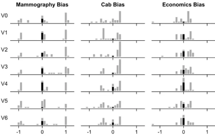
We start with an analysis of BIAS, which captures the discrepancy between the subjects’ answers to the problems and the exact answers. Figure 2 shows the distributions of BIASper PROBLEMand VISfor the 24 subjects assigned to each VIScondition.

From Figure 2, it can be observed thati)consistent with previous findings [27], answers are not normally distributed, certain wrong an-swers being much more common than others;ii)the distributions dif-fer across PROBLEMs but seem very similar across VISconditions. In particular, there is no obvious sign of V1-V6 outperforming V0.

The distributions are also well-balanced around zero, suggesting no clear general tendency to underestimate or overestimate probabilities. Median biases per PROBLEM×VISwere overall close to zero (for all 21 values of median biasesM=0.06,SD=0.13), as well as mean biases (M=0.003,SD=0.14). A grand mean of 0.003 is remarkably small (it would correspond to a probability estimate of, e.g., 0.1007 instead of 0.1) and suggests a “wisdom of the crowd” effect [52].

Bias Bias Mammography Bias V0 Bias Bias Cab Bias Bias Bias Economics Bias Bias Bias V1 Bias

Bias BiasBias

Bias Bias V2

Bias

Bias BiasBias

Bias Bias V3

Bias

Bias BiasBias

Bias Bias V4

Bias

Bias BiasBias

Bias Bias V5

Bias

Bias BiasBias

-1 0 1

V6

-1 0 1 -1 0 1

Fig. 2. Distributions of bias in answers per Bayesian problem and visu-alization condition (N=24each). Black bars are exact answers. A bias of−1means an answer10×lower and a bias of1means10×higher.

4.5.2 Exact Answers and Errors

Exact answers are those for which EX= 1 or equivalently, BIAS= 0. They are shown in Figure 2 as black bars. There were 12% ex-act answers overall, with 15% exex-act answers forMam, 5% forCab and 15% for Eco. V0 yielded 6% exact answers, whereas V1-V6 yielded 14%,11%,11%,21%,7% and 14% exact answers (N =24 each). These percentages are much lower than in previous studies, suggesting that the problem does not lie in a systematic bias (e.g., no evidence for a base rate fallacy), but rather in poor individual accuracy. A finer measure of accuracy is the ERRORmetric, i.e., how far the answers were to correct answers. The overall median ERRORwas 0.27 (M=0.38,SD=0.39). A mean of 0.38 is fairly large and corresponds to a probability estimate of, e.g., 0.24 or 0.04 instead of 0.1.

4.5.3 Effect of Visualization on Error

In the rest of this section, we average the errors forMam,CabandEco into a single ERRORmeasure. Box plots of ERRORper VISare shown in Figure 3. It can be seen that effect sizes are quite small (differences in medians are much smaller than variances) and, a Kruskal-Wallis rank sum test for non-normal distributions indeed reports no signifi-cant difference between VISconditions (H(6) = 4.1,p=0.66). Thus, our hypothesis H1b (V2 is more accurate than V1) is not confirmed.

Comparing text alone with all V1-V6 aggregated (N=144) does not yield any significant difference either (Kruskal-Wallis, H(1) = 1.6,

p=0.21). Thus, our hypothesis H1a cannot be confirmed either. 4.5.4 Subject Abilities

The median score for numeracy NUMwas 24 / 30 (M=23.5,SD=

4.0), while that for spatial ability SPATwas 5 / 10 (M=5.1,SD=2.2). More than half (55%) the subjects got a moderate to high score for both tests, as defined by [9, 23]. Correlations between ERRORand subject abilities were low (r=−0.08 for NUM and r=−0.07 for SPAT), suggesting little influence of abilities on accuracy overall.

We conducted further analyses by splitting subjects into two groups: SPAT≤5 and SPAT>5. In both groups, mean errors were very similar (M∈[0.36, 0.38]) for V0, glyph-based visualizations combined (V3-V6) and Euler-based visualizations combined (V2 and V4-(V3-V6), with no statistically significant difference. Thus, our hypotheses H1c and H1d on effects of individual abilities are not confirmed.

4.5.5 Confidence in Answers

The median score for CONFwas 3 on a 5-point Likert scale (M=3.4, SD=1.1): subjects were typically “reasonably confident” in their an-swers, with a trend towards high confidence. Correlation with ERROR

was low (r=−0.08). Medians for CONFaveraged across problems ranged from 3.0 to 3.7 depending on the VIScondition, with no statis-tically significant difference (Kruskal-Wallis, H(6) = 5.8,p=0.45).

0.0 0.2 0.4 0.6 0.8 1.0 1.2 Combined Error V6 V5 V4 V3 V2 V1 V0

Fig. 3. Answer errors for all three Bayesian problems combined per visualization condition (N=24each).

4.5.6 Time Spent

The median completion time for reading and answering problems (TIME) was 113 sec (M=154 sec,SD=130): subjects typically spent about 2 min on each problem, which is about half the time spent by our initial pilot subjects (researchers and students from our laboratories). The correlation with ERRORwas low (r=0.02). The median TIME

for the first problem presented was 129 sec and went down to 106 sec for the last one, suggesting a moderate learning effect.

An analysis of variance (ANOVA) with the modellog(TIME)∼VIS

suggests that the total time spent on the three problems depends on the VIScondition (F(6, 161) = 2.5,p< .05). Post-hoc pairwise compar-isons witht-test and Bonferroni correction reveal a difference between V1 and V2 and between V2 and V4 (p< .05). Median times were 168 sec for V1, 72 sec for V2 and 149 sec for V4. Thus, although subjects were not more accurate with V2 than V1 (our initial hypothesis H1b), they spent much less time (less than half) parsing V2.

4.6 Qualitative Feedback

When asked which tools or methods they used to get their answer, 8% of the participants specifically reported using Bayes’ theorem (not mentioned in the question). Others used basic mathematics, carried out mental calculations, estimated answers, or guessed. About 75% reported using pen and paper or a calculator. Three subjects (2%) commented that they did not know they could use any of these tools.

Three weeks after the experiment, all participants were invited to complete a 2-minute follow-up questionnaire for $0.20 on MTurk. Fifty-three participants out of the 168 (32%) responded. The seven vi-sualization types for theCabproblem were shown and the participants had to either identify the type they had seen during the experiment or state that they do not remember at all. They then had to indicate on a 5-point Likert scale how much they looked at the provided visualiza-tions, how much they used them to solve the corresponding problems, and explain why. This helped us understand whether the participants referred to the visualizations and whether they found them helpful.

A large majority (89%) of the 53 respondents reported using the visualizations to solve the problem (scales 3-‘somehow used them’ up to 5-‘used them a lot’ on a 5-point Likert scale). However, only 47% remembered the correct visualization type. This was likely due to the relatively long time period between the experiment and the ques-tionnaire and, due to the similarities among some visualization types. Among those who correctly remembered the visualization type, 92% reported using the visualization to solve the problem.

Most of the 53 respondents (79%) commented that the diagrams helped them visualize the problem (e.g., Table 3a), of which 6 (11%) specifically indicated that it helped them understand the relationships between the sets and the given values (e.g., Table 3b). Four subjects (8%) who had text alone (V0) wished they had diagrams (e.g., Table 3c). Five (9%) reported comparing the color and size of the sets and the overlapping regions, while 3 (6%) reported counting the glyphs. Other positive comments included: the diagrams helped to understand the statistics (e.g., Table 3d), clarified the problem (e.g., Table 3e), helped to identify the regions for the final answer (e.g., Table 3f).

Table 3. Some participant comments in the follow-up questionnaire.

a It can be explained only if there is a diagram relevant to the incident or question. b Diagrams show relationships between different sets. Easy to understand links. c I had trouble visualizing the data on my own. Diagrams would have been essential. d Diagrams gave me a visual clue to understand problem better and to find answer. e It would have been helpful to picture the scene.

f Saw the diagram and figured out the regions for the answer.

g I compared the size of the circles and the overlapping regions, but just looking at the diagram was not enough.

h Used diagrams to get answer but did not fully understand them so it was difficult. i When thinking about populations, sample sizes and similar statistical problems,

an intuitive grasp of problem comes quicker and easier through diagrams than mere words. I would not, however, have slavishly followed diagrams since I would still have to determine if the diagram was accurate and represented the problem as stated.

j The text was enough, they didn’t simplify anything, just complicated it more. k The text was more than sufficient.

However, 7 participants (13%) commented that the diagrams were not enough to answer the question (e.g., Table 3g). Three (6%) said that they did not fully understand the diagram (e.g., Table 3h), while one reported a lack of familiarity with the visualization. Six (11%) used the diagrams just to verify their answer, 4 (8%) stated that they did not trust the diagrams because in some experiments they are drawn incorrectly on purpose (e.g., Table 3i), while 3 (6%) claimed that hav-ing two representations was confushav-ing and since the actual values were in the text, they ignored the visualization (e.g., Table 3j). Three (6%) stated that the diagrams were useless (e.g., Table 3k).

4.7 Discussion

Though we used the best known textual representation (natural fre-quencies) [27] and the same text and text+visualization format as in previous studies, we failed to replicate previous findings as our sub-jects’ accuracy was remarkably lower. For instance, considering V0 (text and no visualization), previous studies reported 35% [8], 46% [27], 51% [49] and 72% [18] exact answers with the natural frequency format, which are considerably higher than the 6% we obtained.

Yet, everything seems to suggest that our participants completed the tasks seriously. Only workers with a high HIT accept rate (95%) could participate and, since such a selection criteria is common practice, they have incentives to maintain a high rate. In addition, they were overall successful at the tests, the paper folding test being particularly attention-demanding. Finally, they often reported being confident in their answers and wrote a number of positive comments.

Of much concern is the fact that nearly all of our subjects were at least reasonably confident in their answer. In a real world situation, fallacious reasoning combined with overconfidence can easily lead to wrong decisions, with potentially harmful consequences (e.g., choos-ing whether to undertake chemotherapy after bechoos-ing diagnosed with cancer). Since we found that bias was close to zero overall, bad judg-ments could go either way.

We believe that far from invalidating the choice of the crowdsourc-ing method, these poor results motivate the need for more studies of this sort. It is important that techniques that aid probabilistic reason-ing and decision makreason-ing can benefit untrained people with different backgrounds and age ranges and, remain effective in situations where little time and attention are available.

In addition to a low accuracy overall, none of the visualizations we tested seemed to help. Although there is surely an effect [14], Fig-ure 3 suggests that effects on our metrics of interest (see Section 3.4) are small. This contrasts with conclusions drawn from studies on pro-portions of correct answers [8]. Girotto and Gonzalez go as far as arguing that with appropriate use of visualizations, anyone (including ‘naive’ subjects) could solve Bayesian problems [28]. However, our results are also consistent with previous studies finding no significant improvement with visualizations over text alone [18].

Although Cosmides and Tooby suggest that passive visualizations are ignored when solving Bayesian problems [18], 89% of our 53

par-ticipants who completed the follow-up questionnaire confirmed that they at least “somehow” used the diagram. Most of them reported finding the diagram very useful and commented that they generally like being given diagrams to solve problems. So it seems that subjects tended to overestimate the degree to which diagrams are helpful.

It is worth noting that despite positive comments overall, various participants commented that they did not fully understand the diagram, that having two representations was confusing, that they ignored it and that the information provided in the text was sufficient. A few others doubted the credibility of the diagram and chose to trust the text.

Several solutions have already been suggested. Teaching Bayesian reasoning is one of them. It can be extremely effective [48] but again, we chose to focus on techniques that can be used without prior train-ing or background. Another well known approach is the use of active rather than passive visualizations [18] (but see also [8]). Having peo-ple draw their own visualization can be effective, but it is not practi-cal in many situations, including in scientific press, informative pam-phlets, or in broadcasted visual adverts [26]. For similar reasons, static visualizations should probably be considered before interactive ones.

Since the answer to the Bayesian problem is in the diagram itself, it should be possible to increase the chances that people find it, either by i)helping them make the link between the text and the diagram [28]; ii)encouraging them to search for the solution in the diagram; andiii) forcing them to search for the solution in the diagram.

We propose two alternative presentation techniques that only in-volve moderate modifications to the text:a)adding short instructions in the text that refer to the diagram (thereby supportingiand possibly ii),b)removing all numerical quantities from the text (supportingiii). The last technique is based on the idea that a rough estimation can be better than a plain wrong calculation and should further eliminate any possible doubt that the visualization is not credible.

We conducted a second experiment in order toi)confirm that simply adding a visualization to a Bayesian problem is of little help, andii) testing whether an improvement can be obtained by the above two presentation techniques. In order to testi, we only included V0 and V4 and increased statistical power with larger sample sizes (fromN=24 toN=120 each). V4 was the diagram with the lowest mean error and combined both Euler diagrams and glyphs. To further simplify the design, we only included theMamproblem. We chose it because it is a classic problem which has been used in various studies [21, 27].

5 EXPERIMENT2: ALTERNATIVETEXTFORMATS

In this second experiment, we set ourselves toi)confirm with a larger sample that simply adding a visualization to a Bayesian problem is of little help, andii)investigate some possible solutions.

Based on the data from our first experiment, we hypothesized that simply appending a visualization to the textual information will yield at best weak improvements (our data only shows non-significant dif-ferences in mean ERRORs of about 0.1 points). We further hypothe-sized that this issue could be addressed by providing instructions in the text on how to parse the visualization. We also believed that the numerical values provided in the text could encourage wrong calcu-lations and discourage parsing the visualization, so we hypothesized that not providing these values would also help.

5.1 Design

Our independent variable was presentation type PRES, with the fol-lowing four conditions:

• V0: Textual form only, equivalent to the condition{PROBLEM= Mam, VIS= V0}from the previous experiment;

• V4: Text with visualization, equivalent to the previous condition

{PROBLEM=Mam, VIS= V4};

• V4a: Like V4, but with references to the visualization in the text (Table 4);

• V4b: Like V4, but with numbers removed from the text (Table 4). We used a between-subjects design and our dependent variables were BIAS, ERROR, EX, TIMEand CONFas previously.

Table 4. Novel text formats for theMamproblem in experiment 2.

V4a 10 out of every 1,000 women at age forty who participate in routine screening have breast cancer(compare the red dots in the diagram below with the total number of dots). 8 of every 10 women with breast cancer will get a positive mammography (compare the red dots that have a black border with the total number of red dots). 95 out of every 990 women without breast cancer will also get a positive mammography (compare the blue dots that have a black border with the total number of blue dots). V4b A small minority of women at age forty who participate in routine screening have breast cancer. A large proportion of women with breast cancer will get a positive mammography. A small proportion of women without breast cancer will also get a positive mammography.

5.2 Participants

Our participants were 480 MTurk workers who never completed any of our previous HITs. We thought the demographics should be similar to the previous experiment (Section 4.2), so we did not include any demographics questions.

5.3 Procedure

We conducted the experiment on MTurk as previously. The HITs were shorter, including only theMamproblem and no abilities tests.

5.3.1 Task

The form was made up of four pages and took around five minutes to complete. After the instruction page, theMamproblem was presented using either V0, V4, V4a or V4b. The questions and the layout of the pages were the same as before, except participants were told they could optionally use any tool or method. The next page had a single catch question. On the final page, participants were asked whether they tried to compute an exact answer and had to indicate on a 5-point Likert scale how much they used the diagram to solve the problem.

5.3.2 MTurk Design

We created four unique HITs, one for each presentation condition, and 120 assignments for each were uploaded on MTurk with a $0.40 re-ward. The same system qualification was used as in Experiment 1. Participants to Experiment 1 were blocked and duplicate HITs were rejected as before. HITs of workers who selected the wrong answer to the catch question were also rejected. In contrast to the previous experiment, workers who submitted the HIT only once but had previ-ously seen the problem (either because they gave up before submitting or experienced technical issues) were identified through a question on the last page asking the workers whether they already attempted to load the HIT but failed to submit it. We clearly stated that this was not going to affect our decision to accept or reject the HIT. In fact, HITs from workers who replied “yes” or “unsure” (about 11%, not included inN=480) were accepted (i.e., paid) and the data was discarded from analysis.

5.4 Hypotheses

Our hypotheses were:

• H2a. Condition V4 does not lower the mean ERRORby more than 0.1 points compared to V0,

• H2b. Condition V4a yields lower ERRORs than V4, • H2c. Condition V4b yields lower ERRORs than V4.

5.5 Results

5.5.1 Bias

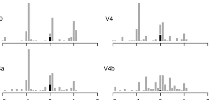
Figure 4 shows the distributions of BIASfor each PRES. These are similar to those of the previous experiment, except for V4b which is closer to normal. This time, as shown in Figure 5, not all the distribu-tions were well-balanced around zero. The median biases were 0.015, -0.59, -0.49 and 0.013 for V0, V4, V4a and V4b. The differences are statistically significant (Kruskal-Wallis, H(3) = 22,p< .001).

Bias Bias Mammography Bias V0 Bias Bias V4 −2 −1 0 1 2 V4a −2 −1 0 1 2 V4b

Fig. 4. Distributions of biases in answers to theMamproblem (N=120 each) per presentation type. Black bars are exact answers.

● ● ● −2 −1 0 1 Mammography Bias V4b V4a V4 V0

Fig. 5. Biases in answers to theMamproblem per presentation type (N=120each). ● ● ● ● ● ● ● ● ● 0.0 0.5 1.0 1.5 2.0 2.5 Mammography Error V4b V4a V4 V0

Fig. 6. Answer errors to theMamproblem per presentation type (N=120 each).

5.5.2 Accuracy

Exact answers for V0 and V4 were 3.3% and 5.0% (see black bars in Figure 4) and lower than in the previous experiment (15% forMam). Median errors for V0 and V4 were both 0.8903 and equal to those of the previous experiment. Mean errors were however larger (0.76 and 0.68 compared with 0.64 and 0.54 for the previous experiment). Thus, it seems that subjects were overall less successful in this experiment.

That V4 yielded a lower mean error than V0 suggests that adding a diagram might have helped, but the difference in means is consistent with H2a (0.68 vs. 0.76 and same medians). Inconsistent with H2b however, V4a yielded the same ratio of exact answers, the same me-dian error and a similar mean error as V4, suggesting that referring to the diagram in the text did not help. In contrast, although V4b rarely yielded an exact answer3 (0.83%), it yielded a much lower median error of 0.41 and a lower mean error of 0.53, consistent with H2c.

The differences between PREStypes, shown in Figure 6, are statis-tically significant (Kruskal-Wallis, H(3) = 21, p< .001). A multiple comparison with V0 using Siegel and Castellan’s procedure reveals that all visual presentation types are significantly better than text alone, confirming our previous hypothesis H1a (R package kruskalmc, one-tailed, p< .05). Using the same test with V4 as the control, the only

3_{A single subject out of 120 gave the exact answer. Later in the}

question-naire, this subject commented, “I kept losing count, so I hit PrintScreen, and pasted it into paint, and marked the ones I had counted.”

significant difference is with V4b, confirming our hypothesis H2c (re-moving numbers helps) but not H2b (referring to the figure helps). Fi-nally, a Wilcoxon test of equivalence for non-normal data confirms our hypothesis H2a (R package etc.diff, margins= [−0.1,0.1],p< .05).

Hence, all visual presentations were better than text alone but im-provements were small, except for V4b where imim-provements were larger. The task involved in V4b was still error-prone, with proba-bility estimations typically about 3 times lower or higher, but it clearly improved over V0 for which typical estimates were 6 or 8 times lower or higher (depending on whether we consider the average or the me-dian error). In addition, V4b yielded no bias, whereas with other visual presentations subjects tended to underestimate probabilities.

5.5.3 Confidence

Confidence scores were similar to before and very similar across PRES, with a median of 3 (“reasonably confident”) and means between 3.28 and 3.36. Differences were not statistically significant (Kruskal-Wallis, H(3) = 0.6,p=0.89). As before, correlation with error was low (r=−0.06).

5.5.4 Time

Completion times were similar to those of the previous experiment and similar across all PRES conditions (ANOVA, F(3, 476) = 1.26, p=0.29). Medians ranged from 112 sec for V4b (M=145,SD=115) to 132 sec for V4a (M=163,SD=108).

5.5.5 Strategies

Discarding “unsure” responses (9% overall), subjects who reported having tried to get the exact answer were 68%, 72%, 63% and 50% for V0, V4, V4a and V4b. This suggests that diagrams did not dissuade subjects from trying to find the exact answer.

As for the degree to which subjects reported relying on the diagram, the median answer to the 5-point Likert scale was 3 for V4 (M=3.3, SD=1.5). Subjects who were assigned to V0 and later asked whether they would have used the diagram gave a median answer of 4 (M=3.6, SD=1.), suggesting that subjects tend to use diagrams less than they would have predicted.

V4a was similar to V4, with a median answer of 3.5 (M=3.4,SD=

1.3). In contrast, the median answer was 5 for V4b (M=4.4,SD=

0.86). This indicates that, rather unsurprisingly, subjects relied on the diagram much more when numbers were not provided.

5.6 Discussion

Our first experiment revealed that crowdsource workers were quite un-successful at solving Bayesian problems. Our second experiment had two objectives: i)confirm that simply adding a Euler/Glyph visual-ization to a Bayesian problem is not a viable solution (we increased sample size fromN=24 toN=120 to get more statistical power) and ii)start exploring possible solutions to this problem.

We met our first objective by measuring a statistically significant difference between text alone and text+diagram, but showing that the practical difference was small (no more than 0.1 points of mean error as confirmed by an equivalence test).

We incidentally found that subjects were even less accurate than in our previous experiment, although the reasons for this are unclear. The design differed in two respects: a)subjects were initially instructed they could use any tool but they did not have to; b) those who re-ported having previously seen the HIT without submitting were dis-carded from the analysis (11%). So subjects might have been primed in trying to get exact answers and failed in their calculations, or alter-natively, our previous experiment could have overestimated subjects’ accuracy by including workers who possibly acquainted themselves with the problem way before carrying out the task.

With respect to our second objective, we tried two alternative pre-sentations and found that referring to the diagram within the text (V4a) did not help, whereas removing the actual numbers from the text (V4b) yielded clear improvements. This is an important finding, since it is a simple and effective technique that can be easily applied to many real-life situations. Previously proposed techniques are more difficult to

apply since they either involve prior training, or like active construc-tions, they require a pen and paper, time and possibly assistance [18]. We do not know of any previous study on Bayesian reasoning which proposed a technique similar to V4b, possibly due to the fact that most of them focused on increasing the number of exact answers rather than reducing estimation errors.

Our particular study focused onhowto reduce inaccuracy, exclud-ing investigations onwhyexactly subjects make mistakes andwhat these mistakes are. Some previous studies have observed different types of miscalculations in Bayesian reasoning tasks [27] and such investigations are likely crucial for designing effective visualizations and text formats. The distributions in Figure 4 do suggest that typical miscalculations or reasoning errors have occurred in our experiments. Some of them (close to bias 1) seem less common when a visualization is provided, possibly resulting in more miscalculations of a different type (close to bias -1) and a lower bias overall (Figure 5). Trying to address specific mistakes might help to further increase accuracy, in-cluding when no numbers are provided, since diagrams can be misin-terpreted. However, recurrent mistakes seem to vary across problems (Figure 2) and finding general solutions might be challenging.

Our findings on visualization-friendly textual formats are only an-other step towards helping people being more accurate in Bayesian reasoning: even when shown a diagram without numbers, workers were still inaccurate at estimating probabilities (with a typical esti-mation about 3 times lower or higher). There are further possible im-provements to our presentation techniques, such as showing numbers on the visualization. The text (story) could also be overlaid on the visualization, or alternatively, miniature visualizations could be em-bedded in the text [53]. Although we focused on static representations due to their wider applicability, interactive techniques can not only help users understand the relationship between text and diagrams, but also let them explore variants and generalize the problems [54].

Other directions for future work include extending our design space with other types of Bayesian visualizations and comparing their effi-ciency. Although our initial comparison was inconclusive, we antici-pate that using problem formats that are more adapted to visualizations will encourage subjects to actually use them and will ultimately make these visualization designs easier to compare in terms of both speed and estimation accuracy.

6 CONCLUSION

We used crowdsourcing to assess the effect of six visualizations (based on Euler diagrams, glyphs and combinations of both) on probabilistic reasoning using three classic Bayesian problems in psychology. Our findings were inconsistent with previous studies in that subjects’ ac-curacy was remarkably low and did not significantly improve when a visualization was provided with the text. A follow-up experiment con-firmed that simply adding a visualization to a textual Bayesian prob-lem is of little help for crowdsource workers. It however revealed that communicating statistical information with a diagram, giving no num-bers and using text to merely set the scene significantly reduces prob-ability estimation errors. Thus, novel representations that holistically combine text and visualizations and that promote the use of estimation rather than calculation need to be investigated.

We also argue for the need to carry out more studies in settings that better capture real-life rapid decision making than laboratories. We propose the use of crowdsourcing to partly address this concern, as crowdsourcing captures a more diverse and less intensely focused pop-ulation than university students. Doing so, we hope that appropriate representations that facilitate reasoning for both laymen and profes-sionals, independent of their background, knowledge, abilities and age will be identified. By effectively communicating statistical and prob-abilistic information, physicians will interpret diagnostic results more adequately, patients will take more informed decisions when choos-ing medical treatments, and juries will convict criminals and acquit innocent defendants more reliably.

ACKNOWLEDGMENTS

REFERENCES

[1] I. Ajzen. Intuitive theories of events and the effects of base-rate informa-tion on predicinforma-tion. Personality and Social Psychology, 35(5):303–314, 1977.

[2] J. S. Ancker, E. U. Weber, and R. Kukafka. Effect of arrangement of stick figures on estimates of proportion in risk graphics. Medical Decision Making, 31(1):143–150, 2011.

[3] M. Bar-Hillel. The base-rate fallacy in probability judgments. Acta Psy-chologica, 44(3):211–233, 1980.

[4] A. K. Barbey and S. A. Sloman. Base-rate respect: From ecological rationality to dual processes.Behavioral and Brain Sciences, 30(3):241– 254; discussion 255–297, 2007.

[5] A. K. Barbey and S. A. Sloman. Base-rate respect: From statistical for-mats to cognitive structures.Behavioral and Brain Sciences, 30(3):287– 297, 2007.

[6] M. I. Bauer and P. N. Johnson-Laird. How Diagrams Can Improve Rea-soning.Psychological Science, 4(6):372–378, 1993.

[7] F. Benoy and P. Rodgers. Evaluating the Comprehension of Euler Dia-grams. InConf Information Visualization (IV), pages 771–778, 2007. [8] G. L. Brase. Pictorial representations in statistical reasoning. Applied

Cognitive Psychology, 23(3):369–381, 2009.

[9] S. Brown, J. Culver, K. Osann, D. MacDonald, S. Sand, A. Thornton, M. Grant, D. Bowen, K. Metcalfe, H. Burke, M. Robson, S. Friedman, and J. Weitzel. Health literacy, numeracy, and interpretation of graph-ical breast cancer risk estimates. Patient Education and Counseling, 83(1):92–98, 2011.

[10] K. Burns. Painting pictures to augment advice. InConf Advanced Visual Interfaces, pages 344–349, 2004.

[11] G. B. Chapman and J. Liu. Numeracy, frequency, and Bayesian reason-ing.Judgment and Decision Making, 4(1):34–40, 2009.

[12] J. J. Chen, N. J. Menezes, A. D. Bradley, and T. A. North. Opportuni-ties for Crowdsourcing Research on Amazon Mechanical Turk. Human Factors, 5:3, 2011.

[13] Chicago Tribune. A false hiv test caused 18 months of hell, (3/5/1993). [14] J. Cohen. The Earth is Round (p <.05). American Psychologist,

49(12):997–1003, 1994.

[15] W. G. Cole. Understanding Bayesian reasoning via graphical displays. In ACM Conf Human Factors in Computing Systems, pages 381–386, 1989. [16] W. G. Cole and J. E. Davidson. Graphic Representation Can Lead To Fast and Accurate Bayesian Reasoning. InSymp Computer Application in Medical Care, pages 227–231, 1989.

[17] C. Collins, G. Penn, and S. Carpendale. Bubble sets: revealing set rela-tions with isocontours over existing visualizarela-tions.IEEE Transactions on Visualization and Computer Graphics, 15(6):1009–1016, 2009. [18] L. Cosmides and J. Tooby. Are humans good intuitive statisticians after

all? Rethinking some conclusions from the literature on judgment under uncertainty.Cognition, 58(1), 1996.

[19] T. C. Davis, N. C. Dolan, M. R. Ferreira, C. Tomori, K. W. Green, A. M. Sipler, and C. L. Bennett. The role of inadequate health literacy skills in colorectal cancer screening.Cancer Investigation, 19(2):193–200, 2001. [20] J. G. Dolan and S. Iadarola. Risk communication formats for low proba-bility events: an exploratory study of patient preferences.BMC Medical Informatics and Decision Making, 8(14):14, 2008.

[21] D. M. Eddy.Probabilistic reasoning in clinical medicine: problems and opportunities, pages 249–267. Cambridge University Press, 1982. [22] R. B. Ekstrom, J. W. French, H. H. Harman, and D. Dermen.Manual for

Kit of Factor-Referenced Cognitive Tests. Educational Testing Service, 1976.

[23] A. Fagerlin, B. J. Zikmund-Fisher, P. A. Ubel, A. Jankovic, H. A. Derry, and D. M. Smith. Measuring numeracy without a math test: development of the Subjective Numeracy Scale.Medical Decision Making, 27(5):672– 80, 2007.

[24] M. Galesic, R. Garcia-Retamero, and G. Gigerenzer. Using Icon Arrays to Communicate Medical Risks: Overcoming Low Numeracy. Health Psychology, 28(2):210–216, 2009.

[25] G. Gigerenzer. Ecological intelligence: An adaptation for frequencies, volume 39, pages 9–29. Oxford University Press, 1998.

[26] G. Gigerenzer, W. Gaissmaier, E. Kurz-Milcke, L. M. Schwartz, and S. Woloshin. Helping Doctors and Patients Make Sense of Health Statis-tics.Psychological Science in the Public Interest, 8(2):53–96, 2007. [27] G. Gigerenzer and U. Hoffrage. How to Improve Bayesian

Reason-ing Without Instruction: Frequency Formats. Psychological Review, 102(4):684–704, 1995.

[28] V. Girotto and M. Gonzalez. Solving probabilistic and statistical

prob-lems: a matter of information structure and question form. Cognition, 78(3):247–276, 2001.

[29] I. J. Good. When batterer turns murderer.Nature, 375(6532):541, 1995. [30] J. Heer and M. Bostock. Crowdsourcing Graphical Perception: Using

Mechanical Turk to Assess Visualization Design. InACM Conf Human Factors in Computing Systems, pages 203–212, 2010.

[31] U. Hoffrage and G. Gigerenzer. How to Improve the Diagnostic Infer-ences of Medical Experts. Experts in Science and Society, pages 249– 268, 2004.

[32] U. Hoffrage, S. Lindsey, R. Hertwig, and G. Gigerenzer. Medicine: Com-municating statistical information.Science, 290(5500):2261–2262, 2000. [33] P. N. Johnson-Laird, P. Legrenzi, V. Girotto, M. S. Legrenzi, and J. P. Caverni. Naive probability: a mental model theory of extensional reason-ing.Psychological Review, 106(1):62–88, 1999.

[34] D. Kahneman, P. Slovic, and A. Tversky. Judgment Under Uncertainty: Heuristics and Biases. Cambridge University Press, 1982.

[35] V. Kellen, S. Chan, and X. Fang. Facilitating conditional probability prob-lems with visuals. InConf Human-Computer Interaction, pages 63–71, 2007.

[36] J. J. Koehler. One in Millions, Billions and Trillions: Lessons from Peo-ple V. Collins (1968) for PeoPeo-ple V. Simpson (1995). Legal Education, 47:214–223, 1997.

[37] K. Koffka.Principles of Gestalt Psychology. Harcourt, Brace, 1935. [38] L. Micallef and P. Rodgers. Drawing Area-Proportional Venn-3

Dia-grams Using Ellipses. Technical Report TR-3-11, School of Computing, University of Kent, UK, 2011. http://www.eulerdiagrams.org/eulerAPE. [39] A. L. Nichols and J. K. Maner. The good-subject effect: investigating

par-ticipant demand characteristics. General Psychology, 135(2):151–165, 2008.

[40] G. Paolacci, J. Chandler, and P. G. Ipeirotis. Running experiments on Amazon Mechanical Turk. Judgment and Decision Making, 5(5):411– 419, 2010.

[41] E. C. Poulton and P. R. Freeman. Unwanted asymmetrical transfer effects with balanced experimental designs. Psychological Bulletin, 66(1):1–8, 1966.

[42] M. Price, R. Cameron, and P. Butow. Communicating risk informa-tion: the influence of graphical display format on quantitative information perception-accuracy, comprehension and preferences.Patient Education and Counseling, 69(1-3):121–128, 2007.

[43] N. H. Riche and T. Dwyer. Untangling Euler Diagrams. IEEE Transac-tions on Visualization and Computer Graphics, 16(6):1090–1099, 2010. [44] P. Rodgers, L. Zhang, and A. Fish. General Euler Diagram Generation.

InConf Diagrams, LNCS (LNAI) 5223, pages 13–27, 2008.

[45] P. Rodgers, L. Zhang, and H. Purchase. Wellformedness Properties in Euler Diagrams: Which Should Be Used?IEEE Transactions on Visual-ization and Computer Graphics, 18(7):1089–1100, 2012.

[46] J. Ross, L. Irani, M. S. Silberman, A. Zaldivar, and B. Tomlinson. Who are the Crowdworkers? Shifting Demographics in Mechanical Turk. In ACM Conf Human Factors in Computing Systems, pages 2863–2872, 2010.

[47] T. A. Salthouse. The processing-speed theory of adult age differences in cognition.Psychological Review, 103(3):403–428, 1996.

[48] P. Sedlmeier and G. Gigerenzer. Teaching Bayesian reasoning in less than two hours.Experimental Psychology General, 130(3):380–400, 2001. [49] S. A. Sloman, D. Over, L. Slovak, and J. M. Stibel. Frequency illusions

and other fallacies. Organizational Behavior and Human Decision Pro-cesses, 91(2):296–309, 2003.

[50] G. Stine. Acquired immune deficiency syndrome: biological, medical, social, and legal issues. Prentice Hall, 1996.

[51] E. R. Stone, J. F. Yates, and A. M. Parker. Effects of numerical and graph-ical displays on professed risk-taking behavior.Experimental Psychology Applied, 3(4), 1997.

[52] J. Surowiecki.The Wisdom of Crowds. Anchor, 2005. [53] E. R. Tufte.Beautiful Evidence. Graphics Press, 2006.

[54] B. Victor. Explorable Explanations. http://worrydream.com, 2011. [55] H. G. Welch and W. C. Black. Overdiagnosis in Cancer. J National

Cancer Institute, 102(9):605–613, 2010.

[56] L. Wilkinson. Exact and Approximate Area-proportional Circular Venn and Euler Diagrams.IEEE Transactions on Visualization and Computer Graphics, 18(2):321–331, 2011.

[57] K. Yamagishi. Facilitating normative judgments of conditional probabil-ity: frequency or nested sets? Experimental Psychology, 50(2):97–106, 2003.

[58] P.-H. Zahl and J. Maehlen. Overdiagnosis in mammography screening. Tidsskr Norske Laege, 124(17):2238–2239, 2004.