M e t h o d o l o g i e s a n d
W o r k i n g p a p e r s
ISSN 1977-0375
Statistical matching: a model based approach
for data integration
2013
edition
M e t h o d o l o g i e s a n d
W o r k i n g p a p e r s
Statistical matching: a model based approach
for data integration
Europe Direct is a service to help you find answers to your questions about the European Union.
Freephone number (*):
00 800 6 7 8 9 10 11
0H
(*) The information given is free, as are most calls (though some operators, phone boxes or hotels may charge you).
More information on the European Union is available on the Internet (http://europa.eu). Cataloguing data can be found at the end of this publication.
Luxembourg: Publications Office of the European Union, 2013 ISBN 978-92-79-30355-5
ISSN 1977-0375 doi:10.2785/44822
Cat. No: KS-RA-13-020-EN-N
Theme: General and regional statistics Collection: Methodologies & Working papers © European Union, 2013
Authors:
Aura LEULESCU (Eurostat) Mihaela AGAFIŢEI (Eurostat)
Acknowledgements:
This work was done under the responsibility of Bettina KNAUTH, Head of Unit “Social statistics - Modernisation and Coordination” and Jean-Louis MERCY, Head of Unit “Quality of Life”.
Appreciation goes to the production units in Eurostat Directorate F (Social Statistics) for their comments and support.
We thank also Pilar MARTÍN-GUZMÁN, Francisco FABUEL, Juan MARTINEZ (Devstat) for their input on Chapter 2 - Quality of Life.
Special thanks are due to the members of the ESSNet on Data Integration, for their constant guidance.
The views expressed in this publication are those of the authors and do not necessarily reflect the opinion of the European Commission.
Table of contents
Table of contents
Introduction 7
1 A methodological overview and implementation guidelines 10
1.1 Short introduction to statistical matching 10
1.2 Statistical matching – a stepwise approach in an applied context 12
1.2.1 Harmonisation and reconciliation of multiple sources 12
1.2.2 Analysis of the explanatory power for common variables 15
1.2.3 Matching methods 16
1.2.4 Quality assessment 19
1.3 Concluding remarks 24
2 Case study 1: Quality of Life 28
2.1 Background 28
2.2 Statistical matching: methodology and results 30
2.2.1 Harmonisation and reconciliation of sources 30
2.2.2 Analysis of the explanatory power for common variables 33
2.2.3 Matching methods 37
2.2.4 Results and quality evaluation 38
2.3 Conclusions and Recommendations 43
Annex 2-1 Common variables- metadata analysis 45
Annex 2-2 Coherence analysis: comparison confidence intervals for marginal distributions of
common variables (EQLS-SILC 2007) 55
Annex 2-3 Analysis explanatory power of common variables: Rao-Scott tests results
(EQLS, 2007) 66
3 Case study 2: Wage and labour statistics 70
3.1 Background 70
3.2 Statistical matching: methodology and results 70
3.2.1 Harmonisation and reconciliation of sources 70
3.2.2 Analysis of the explanatory power for common variables 73
3.2.3 Matching methods 74
3.2.4 Results and quality evaluation 74
3.3 Conclusions and Recommendations 83
Annex 3-1 Common variables- metadata analysis 84
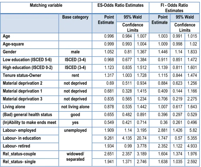
Annex 3-2 Model log(wage) as dependent variable, Spain 2009 89
Annex 3-3 Comparison of joint distributions (based on HD) of matching variables with wage deciles (LFS imputed versus EU-SILC observed) for Spain, 2009; 91
Table of contents
Table of content - Box
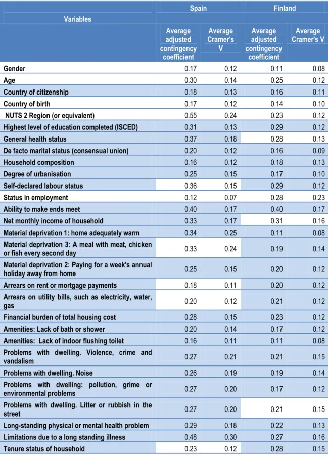
Box 1-1 Statistical matching situation 11 Box 2-1 Main target indicators in EU-SILC 29 Box 2-2 Main target variables in EQLS ─ considered for matching into EU-SILC 30 Box 2-3 Final matching variables for Spain/Finland (method1), EQLS – 2007 35
Box 3-1 Objectives 70
Table of content - Figure
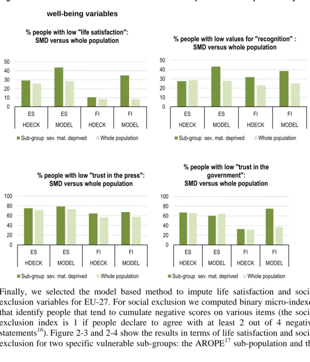
Figure 2-1 Preservation of marginal distributions: observed EQLS versus imputed (%) 39 Figure 2-2 Joint distributions severe material deprivation & imputed subjective well-being
variables 40
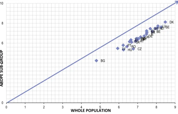
Figure 2-3 Average life satisfaction: whole population versus AROPE 41 Figure 2-4 % people that feel socially excluded: whole population versus materially deprived 41 Figure 3-1 Relative difference in size of target population (employees) between SILC and LFS
based on the self-declared activity status 71 Figure 3-2 The average Hellinger distance by main common variables and by country, in
ascending order 72
Figure 3-3 Average similarity for joint distributions of wage deciles with main socio-demo-
graphical variables, by country 76 Figure 3-4 Impact on predefined cut-off points on wage decile distributions, Greece 2009 77 Figure 3-5 The cut-off points for wage deciles 78 Figure 3-6 Similarity of joint distributions: comparing EU-SILC with LFS observed/imputed
wage data 79
Figure 3-7 Impact of discrepancies in the distribution of main common variables on matching
results 80
Figure 3-8 Mean wage by field of education and age group, ES-2009 81 Figure 3-9 Frechet Bounds: % of people with wage below the mean by field of education
(ES, 2009) 82
Table of content - Table
Table 2-1 Coherence common variables between EU SILC and EQLS, Spain/Finland–2007 32 Table 2-2 Explanatory power common variables for Spain/Finland, EQLS – 2007 34 Table 2-3 Final matching variables for Spain/Finland (dependent variable=life satisfaction),
EQLS — 2007 36
Table 2-4 Frechet bounds for the joint distribution of life satisfaction and severe material
deprivation 42
Table 3-1 Hellinger distance values (%) by country and common variables, in ascending
Introduction
Introduction
Recent initiatives highlighted the growing importance of new indicators and statistical surveillance tools that cover cross-cutting needs and go beyond aggregates to capture key distributional issues. In particular, the ‘GDP and beyond’ Commission communication and the Stiglitz-Sen-Fitoussi Commission’ Report raised awareness about the need to review and update the current system of statistics in order to address new societal challenges and to support policy-making. This urges for integrated statistical information that covers several socio-economic aspects.
The social statistical infrastructure is organised around specific surveys covering many relevant aspects of the users demand: income, consumption, health, education, labour market, social participation. However, no single survey can cover all the requested aspects. Against this backdrop the current process of modernisation of social surveys is focused on increasing the overall efficiency of social surveys, the responsiveness to user needs and the analytical potential of the data collected via a better integrated system of social surveys.
Statistical matching (also known as data fusion, data merging or synthetic matching) is a model-based approach for providing joint statistical information based on variables and indicators collected through two or more sources. The potential benefits of this approach lie in the possibility to enhance the complementary use and analysis of existing data sources (e.g. cross-cutting statistical information that encompasses a broad range of socio economic aspects), without further increasing costs and response burden. However, statistical matching is a complex operation which requires specific technical expertise and raises several methodological issues.
Therefore, in December 2010 in Eurostat started a feasibility study that carried out methodological work with a view to checking whether statistical matching could be used in the framework of social surveys as a tool to integrate extensive information from several existing sources.
The project focused on the ex post integration of existing micro data sets and it had a strong practical focus on specific needs in social statistics. This first publication aims to provide a general overview on the statistical matching methodology and its implementation requirements in a practical context. It has three main objectives: (1) to provide a general introduction to statistical matching with an emphasis on implementation in an applied context, namely within the European system of social surveys; (2) to present the main results and practical highlights from two pilot studies on matching implemented in Eurostat (e.g. producing joint information on quality of life indicators based on EU-SILC1and EQLS2; study the feasibility of the technique for production of tabulated LFS data enhanced with SILC-matched wages); (3) to draw conclusions on the quality of results obtained through statistical matching given the status–quo and translate into recommendations for addressing limitations in the design stage. A second volume on statistical matching is forthcoming. It explores a new approach to statistical matching based on the incorporation of ex-ante requirements in the current process of redesign of social surveys.
1
EU Statistics on Income and Living Conditions 2
Introduction
Chapter 1 reports on the general methodological framework and guidelines for the implementation of matching techniques. Chapters 2-3 document in detail the first empirical case studies conducted in the matching project in Eurostat.
Introduction
1.
1
A methodological overview and
implementation guidelines
1
A methodological overview and
1
A methodological overview and implementation guidelines
1
A methodological overview and
implementation guidelines
1.1 Short introduction to statistical matching
Statistical matching (also known as data fusion, data merging or synthetic matching) is a model-based approach for providing joint information on variables and indicators
collected through multiple sources (surveys drawn from the same population). The potential benefits of this approach lie in the possibility to enhance the complementary use and analytical potential of existing data sources (e.g. cross-cutting statistical information that encompasses a broad range of socio economic aspects). Hence, statistical matching can be a tool to increase the efficiency of use given the current data collections.
Most often the aim of a matching exercise is to enlarge the information scope, but matching techniques have been used also for alignment of estimates observed in multiple surveys and for improving the precision of these estimates by integration with larger surveys.
Two main approaches can be delineated in terms of outputs that can be obtained through matching:
(1) the macro approach refers to the identification of any structure that describes relationships among the variables not jointly observed of the data sets, such as joint distributions, marginal distributions or correlation matrices (D’Orazio, 2006)
(2) the micro approach refers to the creation of a complete micro-data file where data on all the variables is available for every unit. This is achieved by means of the generation of a new data set from two data sets that are based on an informative set of common variables between two ‘synthetic micro records’. An essential feature of statistical matching is that, although the units in the concerned data sets should come from the same population, they are usually not overlapping. You identify and link records from different sources that correspond to similar units. This is the basic difference compared with record linkage, where units included in the data sets overlap that allows to link records from the different data sets that correspond to the same unit. Therefore, record linkage deals with identical units, while statistical matching, or synthetic linkage, deals with ‘similar’ units.
In practice, matching procedures can be regarded as an imputation problem of the target variables from a donor to a recipient survey. Y, Z are collected through two different samples drawn from the same population; X variables are collected in both samples and they are correlated with both Y and Z. The relation between these common variables with the specific variables observed only in one of the data sets - the donor data set- will be explored and used to impute to the units of the other data set - the recipient
1
A methodological overview and implementation guidelines
data set - the variables not directly observed. Thus a synthetic dataset is generated with complete information on X,Y and Z.
Box 1-1 Statistical matching situation
Sample A (donor) Sample B (recipient) Synthetic dataset
X,Y
X,Z X, ,Z
However, this view is rather simplistic and one important methodological concern has been raised regarding the validity of results. The origins of statistical matching can be traced back to the mid- 1960s, when the 1966 US Tax File and the 1967 Survey of Economic Opportunities were matched in order to provide a synthetic data set on socio-demographic variables. Then, in the early 1970s different matching techniques were applied to social surveys in the US (Ruggles 1974), but these techniques were severely criticized on the grounds that they rely on assumptions neither justified nor testable (Kadane 1978, Rodgers 1984). In particular, measures of association between Y and Z conditional on X cannot be estimated and they are usually assumed to be 0. This is the so called conditional independence assumption (CIA), a reference point for assessing the quality of estimates based on matching.
When this condition holds, matching algorithms will produce accurate estimates that reflect the true joint distribution of variables that were collected in multiple sources. It will give the same results as a perfect linkage procedure. Unfortunately, this assumption rarely holds in practice and it cannot be tested from the data sets. In case the conditional independence does not hold, and no additional information is available, the model will have identification problems and the artificial datasets produced may lead to incorrect inferences.
The critical question that arises is: what can we learn from a matched dataset about the joint distribution of (Y, Z), which are not jointly observed? There are two main approaches proposed in current studies on statistical matching that take into account these inherent limitations.
The first one focuses on uncertainty analysis techniques that assess the sensitivity of estimated results to different assumptions (Rubin, 1980; Raessler 2002, D'Orazio et al., 2006). In this case the focus is typically on macro objectives (e.g. estimation of specific contingency tables) rather than the creation of micro-datasets. The second one explores the possibility of overcoming the conditional independence assumption by using auxiliary information. In order to overcome the conditional independence assumption, two main types of solutions were put forward. One is the use of additional information in the form of a small sub-set of units with complete information on the joint distributions (Paass, 1986). The other, which covers cases when the joint collection of specific variables is not feasible, explores the use of proxy ‘variables’ with very high predictive power. These variables can mediate the relationship between Y and Z, and can make plausible the conditional independence assumption.
^ Y
1
A methodological overview and implementation guidelines
In all cases, the focus is on the specific estimators of interest and not on the creation of synthetic datasets (Schaffer, 1998). The matched datasets will not usually preserve individual level values, so the exercise should aim to preserve data distributions and multivariate relations between target variables (Rubin 1986). Therefore, it is essential both to control for dimensions relevant in the analysis and to properly reflect uncertainty associated with implicit models.
In the framework of European official statistics, relevant methodological expertise on statistical matching was developed in the frame of the ESSnet on Data Integration3. The aim of the ESSnet on Data Integration was to promote knowledge and practical application of sound statistical methods for the joint use of existing data sources in the production of official statistics, and at disseminating this knowledge within the European Statistical System. The outputs4 of the project comprise methodological papers and case studies on statistical matching as well as software tools for data integration (Relais for record linkage and StatMatch5 for statistical matching). These tools are written with open source software (mainly R) and are freely available.
1.2 Statistical matching
– a stepwise approach in an applied
context
The application of statistical matching in a practical context usually implies a set of key steps, related to various stages of a survey process. The selection of an appropriate matching technique is only one of these steps and often not the most essential.
First of all, statistical matching relies on certain pre-requisites of harmonisation and coherence of data sources to be matched. Therefore, in practice, it often requires a data reconciliation process that enables the joint analysis of multiple data sources. Secondly, multivariate analysis and modelling techniques need to be implemented for the selection of matching variables. Finally, the application of matching techniques and related quality assessment can be implemented. Every step of the process has to be monitored carefully in order to produce accurate results.
1.2.1 Harmonisation and reconciliation of multiple sources
In order to understand whether data from two different surveys can be matched it is necessary to evaluate if they are coherent. Coherence of the statistics produced by a survey process is an important feature that refers to the adequacy of the data to be reliably combined in different ways and for various uses.
The first step in a data matching process is the harmonisation of multiple sources. An extensive methodological work on harmonisation methods and reconciliation of
3 http://www.cros-portal.eu/content/data-integration-1 4 http://www.cros-portal.eu/sites/default/files//WP2.pdf 5 http://www.cros-portal.eu/sites/default/files//WP3.2%20D%27Orazio%20-%20Updating%20StatMatch%20%28slides%29.pdf
1
A methodological overview and implementation guidelines
multiple sources was done in the framework of the ESSnet on Data Integration. D’Orazio et al (2006) mention the following eight types of reconciliation actions: (a) harmonisation on the definition of units
(b) harmonisation of reference period (c) completion of population
(d) harmonisation of variables (e) harmonisation of classifications
(f) adjustment for measurement errors (accuracy) (g) adjustment for missing data
(h) derivation of variables
Discrepancies can emerge at different levels: in the data collection (e.g. different household definitions, different variables or filters applied to similar variables), but also downstream in the surveys methods (calibration factors or reference sources) and in the derived information disseminated to users (e.g. complex concepts such as household composition, dependent child are calculated based on different criteria).
The empirical studies done in Eurostat showed that in an applied context these standardization issues can hamper the successful application of matching methods. Practical issues, which might arise, and their impact on the quality of matching results are presented in the following sections, based on the different case studies. The single analysis of metadata is not sufficient to understand if data from two surveys can be compared and integrated. This analysis should be followed by data processing of the two surveys.
For example, in sample surveys on households, usually the definition of the household should be deepened in order to understand whether the two surveys share the same definition or not. It is very important to ascertain if all the household members are surveyed or not (e.g. data collected only for member with age >= 18, etc.). These comparisons (e.g. of the household definition) should be accompanied by a comparison of the estimated number of households and their distribution by region, size etc.
An essential point for the quality of results from the matching procedures is the existence of a common set of variables that should be homogeneous in their statistical content. In other words, the two samples A and B should estimate the same distribution for each common variable: the two sample surveys should represent the same population. Common variables selected as matching variables should show similar joint and marginal empirical distributions in the two datasets.
There are different possibilities to quantify the degree of similarity/dissimilarity for different distributions. The first and simplest one is to compute, in the two data sources involved, the weighted frequency distributions for each variable of interest and to calculate the differences. The maximum value of these differences can be taken as a criterion for comparison. Coherence of the variable in the two surveys will be rejected if
1
A methodological overview and implementation guidelines
this maximum difference is higher than a certain threshold. Obviously, this is simply a rule of thumb without much theoretical background, and the threshold established is arbitrary.
Another possibility is to quantify similarity of two distributions so that we could give a relative measure of differences in the distributions of various common variables at different levels. Distance metrics are used to measure distortion of distributions. Thus, we chose the Hellinger distance (see equation below) to quantify the similarity between probability distributions of donor and recipient data. It lies between 0 and 1 where a value of 0 indicates a perfect similarity between two probabilistic distributions, whereas a value of 1 indicates a total discrepancy. Unfortunately, it is not possible to set up a threshold of acceptable values of the distance, according to which the two distributions can be said close. However, a rule of thumb, often recurring in literature, considers two distributions close if the Hellinger distance is not greater than 0.05.
K i R Ri D Di K i N n N n i V p i V p V V HD 1 2 1 2 ' ' 2 1 ) ( ) ( 2 1 ) , (where K is the total number of cells in the contingency table, nDi is the frequency of cell i in the donor data D, nRi is the frequency of cell i in the recipient data R and N is the total size of the specific contingency table.
We applied Hellinger distance because it is easy to interpret and allows for comparisons across variables, surveys and countries. However, Hellinger distance shall be used with cautions since it does not take into account variability due to sampling design or a large number of categories and the thresholds are also set up on arbitrary basis.
The third group refers to statistical tests for the similarity of distributions (Chi square; Kolmogorov Smirnov, Rao-Scott, Wald-Wolfowitz tests). These methods could give a stronger base to the conclusions on similarity/discrepancy between distributions coming from the two sources as they take into account the complex sampling designs applied in social surveys. We have not applied such statistical test because, in Eurostat, the sampling design information is not available for all surveys.
Additionally, when dealing with a continuous X variable, hypothesis testing for comparing of means/totals can be done by considering the usual t-test when an estimate of the sampling errors is available.
When the empirical distributions show substantial differences, some harmonisation procedures can then be applied in order to improve the similarity of the distributions, such as re-categorisations of variables or more complex calibration techniques. There are several studies that focus on the alignment of estimates for common variables in two or more sample surveys based on calibration and re-weighting techniques (Sarndal et al 1992; Renssen and Nieuwenbroek, 1997; Merkouris, 2004). Some of these actions may be difficult to implement, and in some cases, no amount of work can produce satisfactory results.
1
A methodological overview and implementation guidelines
Inconsistencies between surveys can be more prevalent in some countries due to operational differences: similar concepts or common guidelines can be implemented differently in the various countries. Therefore, in the framework of social surveys, the need for coherence must be addressed at different levels of the statistical process. The best possibility of matching occurs when a survey, with a common questionnaire providing some basic information for all the units, is divided into subsamples, each of them containing a module with specific questions answered by the units of that subsample (nested surveys). In this case all the conditions previously mentioned are fulfilled: the population and reference period are the same and the definitions and classifications of the common variables are also identical. Thus, the different modules can be safely matched.
Although good coherence is a necessary pre-condition for matching, it does not address limitations related to the conditional independence assumption. The modelling stage is essential for the quality of estimates obtained in the matching procedure.
1.2.2 Analysis of the explanatory power for common variables
The choice of the matching variables is a crucial point in statistical matching. It was often emphasised (Adamek, 1994) that the choice of suitable matching variables among common variables has a greater impact on the validity of the matching exercise than the matching technique effectively used.
The conditional independence assumption is the reference point. The fulfilment of this condition guarantees that the joint distribution of matched variables Y and Z will be the same as the one obtained from a perfect linkage procedure. This assumption will, consequently, validate inference procedures about the actually unobserved association and induce a strong predictive relationship between the common matching variables and the recipient-donor measures.
This means that the validity of a matching exercise depends to a great extent on the power of the matching variables to behave as good predictors of the specific information to be transferred from the donor to the recipient file.
Optimally, the common variables should contain all the association shared by Y and Z. From this point of view, inclusion of all the common variables in A and B that show some significant relation with the variables to impute would look like a reasonable decision. But it is good to take into account the fact that each additional variable complicates the computational procedure and it can have a negative impact on the quality of results. So, a moderate parsimony in the selection of the matching variables is recommended for practical purposes.
A number of methods can be applied in order to find the optimum set of predictors. Among these methods, multivariate techniques play a fundamental role: stepwise regression as it allows selecting the variables with higher explanatory power for each of the variables in the donor file that will be imputed in the recipient one; factor analysis,
1
A methodological overview and implementation guidelines
that provides rules for the selection of the variables and, finally, the derivation of new common variables with the highest possible explanatory power.
The quality of the variables is a second selection criterion. According to Cibella (2010), it is important to choose as matching variables those with a high level of quality, with no errors and no missing data. On the same line, Scanu (2010) states that it is advisable to avoid the use of highly imputed variables as matching variables. For the implementation of a successful matching process it is fundamental to have good quality reporting on the datasets to be integrated and on the specific procedures of imputation and calibration implemented. It is also necessary to have the imputed values in the dataset appropriately flagged.
The specific analysis to be performed with the matching files can make advisable the inclusion of a small number of variables, called the critical variables, which will be used for the separation of data into groups, the so called “matching classes”, or strata. Then, matching is done independently within strata.
One other issue to consider is that sometimes we need to impute several variables from one dataset to another. However, it is very unlikely that the common variables should have equal explanatory power for each of the specific variables. A common practice is to split the variables to be matched into more or less homogeneous groups, and to perform a statistical matching in each of the groups by using the common variables with the highest explanatory power for that particular group. That generally means using different matching variables, or different weights of these variables for each group. This practice is known as “matching in groups”. It implies that a unit of the recipient set will be most probably matched to a different unit of the donor file for each group of imputed variables.
1.2.3 Matching methods
Many different techniques have been used for statistical matching over more than forty years since these exercises have been implemented. Several strands can be differentiated according to some relevant criteria:
First, there is a clear difference between the techniques that assume conditional independence in the matching data set and those that do not assume it: the techniques belonging to the first group will need only the information contained in the data sets to be matched. If some additional information is available, it will be useful only for checking purposes. On the contrary, the techniques applied to matching exercises in which the conditional independence cannot be assumed are based on the incorporation and use of additional information from the very beginning.
The second classification criterion is connected with the parametric features of the model. If it can be assumed that the joint distribution of variables belongs to a family of known probability distributions (i.e. normal multivariate, multinomial), the matching problem will mainly consist of parameter estimations. That means that it can be solved with parametric techniques, among
1
A methodological overview and implementation guidelines
which the maximum likelihood principle will usually play a fundamental role. If no underlying family of distributions can be specified, non-parametric techniques will have to be used.
Then a third source of classification is the scope given to the concept of statistical matching. Often the goal is to obtain a complete synthetic micro data file through effective imputation of values to the unobserved variables. However, the use of synthetic datasets should be done with caution as imputation approaches have limited ability to recreate individual level values. Therefore, imputed data should be used at a sufficient level of aggregation and for specific estimates, defined and controlled for a priori in the imputation procedure. When only the relationship existing among the two sets of variables is to be explored, macro-matching techniques can be adopted.
Based on these considerations we provide a synthesis of the main matching methods and issues related to their application in a practical context. For more details on the different methods please refer to the outputs of the ESSnet on Data Integration (Working Package 1 of ESSnet-DI , page 42-62) and D’Orazio et al 2006 .
a. Hot deck methods
The most popular matching techniques are, by far, the non-parametric micro-matching methods- to be used under the assumption of conditional independence- known as hot-deck imputation procedures. A common feature of these methods is that they will impute the non-observed variables in the recipient file with “live” values, that is, values really existing in the donor file. A definition of distance is established, and calculated for the common variables. Then each record of the recipient file is associated with the nearest record in the donor file, that is, the record that shows a smallest distance. When two or more donor records are equally distant from the recipient record, one of them is chosen at random. Distance can be defined in many ways. The definitions of distance more frequently employed are the Euclidian distance, the city-block metric or the Mahalanobis distance. A weighted distance can also be adopted, reflecting the relative relevance attributed to each of the matching variables (according to their explanatory power or to any other consideration).
This method is known as unconstrained distance hot deck, unconstrained matching or generalized distance method, and provides the closest possible match. Its main problem is that each record in the donor file can be used as donor more than once, a result that is known as polygamy. Also, some donors can remain unused. The multiple choices of donors can reduce the information and the effective sample size. Also, the empirical distribution of the imputed Z variable in the statistical matching file will usually not be identical to the corresponding distribution in the donor file.
In order to limit the number of times a donor is taken, a penalty weight can be placed on donors already used, while establishing an algorithm that avoids the factor of dependence introduced by the order in which the donor units are taken. Alternatively, a tolerance extra distance can be added to the observed minimum distance, and any units within this distance can be considered as possible matches. Then several devices can be
1
A methodological overview and implementation guidelines
applied for the selection of the final donor. For example, it can be selected at random among the possible choices. It is also usual to impute to the recipient record the average values of all the matches within the established distance, although this method will most probably produce imputed values that will not be “live”, that is, really existing values. The disadvantage of these alternatives to distance hot deck is that they usually increase the average matching distance. Also, when averages are taken, variances and covariances can be underestimated.
Another alternative is the constrained distance hot deck, which allows each record in the donor file to be used only once, provided that the donor file is larger or equal to the recipient file. It consists in finding the best donor for each record by minimizing the distance between records conditioned to the preservation of the weights in both data sets. This ensures that the empirical multivariate distribution of the variables observed only in the donor file is exactly replicated in the synthetic file. When there are more donors than recipients, this method leads to a typical linear programming problem, and its solution usually requires a considerable computational effort.
b. Regression based methods
In a parametric framework, the assumption of conditional independence ensures that data are sufficient to estimate the parameters of the model. Under this assumption the likelihood function of the joint distribution can be calculated as a product of the conditional likelihood functions for each of the data sets and the likelihood function of the marginal distribution of the common variables. Then, maximum likelihood (ML) methods can be employed for the estimation of parameters and the identification of the distribution. Sometimes least square estimators have been employed (Rässler, 2002), which in fact results in a very small difference with the ML estimations for large samples. These methods have several disadvantages: regression towards the mean and sensitivity towards misspecifications of the models. Regression based imputation underestimates the variance of estimates and the results can be very different in comparison with hot deck imputations.
c. Mixed methods
Also, parametric and non-parametric methods are sometimes combined in a two stage process, trying to add to the parsimony of the parametric approach the robustness of non-parametric techniques. Such is the case of the predictive mean matching imputation method (Rubin, 1986) in which, in a first step, the regression parameters of Z on X are estimated on the donor database B. These parameters are used to estimate an intermediate value of Z for each register in the recipient file A. Then, with a suitable distance function, a hot deck method is applied, and the record in B that is nearer to the intermediate value in A is the one used for the final matching. Predictive mean matching is more likely to preserve original sample distributions than expected values. One minor drawback of PPM in this situation is that only “observed” rather than “possible” values can be imputed.
Another interesting mixed method is the propensity score, as described in Rässler (2002). Both data sets are extended with an additional variable taking value 1 for all the records in file A and value 0 for all the records in data set B. Putting both files together,
1
A methodological overview and implementation guidelines
a logit or probit model is estimated, taking as dependent variable the added one, and as independent variables the common variables X (and including the regression constant). The propensity score is defined as the estimated conditional probability of a unit to belong to one of the groups, given X. Then a matching is performed on the basis of the estimated propensity scores: for each recipient record a donor unit is searched with the same or the nearest estimated propensity score.
d. Multiple imputation methods
Multiple imputation techniques are often used in the matching framework in order to address the identification problem of the model. First proposed by Rubin in the 1970′s, the method imputes several values (N) for each missing value, to represent the uncertainty about which values to impute. The pooling of the results of the analyses performed on the multiply imputed datasets implies that the resulting point estimates are averaged over the N implicates and the resulting standard errors and p-values are adjusted according to the variance of the corresponding N sub-samples. This variance called the ‘between imputation variance’, provides a measure of the extra inferential uncertainty due to missing data.
In matching, multiple imputation methods were used to build complete datasets. Used in a Bayesian framework, multiple imputation methods rely on a model for variables with missing data, conditional on both observed variables and some unknown parameters. In these cases, different partial correlations between the two not jointly observed variables are used (CIA is not assumed). These explicit models generate a posterior predictive distribution from which imputations are drawn.
Multiple imputation has been applied mainly in a parametric setting (Moriarty and Scheuren, 2001; Raessler, 2002). It has been used by Rässler (2002) to estimate lower and upper bounds of the unknown parameters. More complex techniques, such as Sequential Regression Multiple imputation account also for complex rooting and different filters in the matched surveys, as well as different models for estimating the missing data (Raghunathan, Reiter and Rubin 2003; Raiter 2004). Some applications for the fully Bayesian model were developed based on several models: normal linear regression model, logistic regression, a Poisson loglinear model, a two stage model for truncated data (the case of wage). These give the flexibility in handling each variable on a case by case basis. The disadvantage is that they can be computationally intense.
1.2.4 Quality assessment
The quality assessment in the context of matching needs a process approach. Each of the steps (the quality and the coherence of data sources, modelling techniques, matching/imputation algorithms) has a large impact on the quality of results. However, given certain pre-requisites in terms of coherence and integration, results obtained through statistical matching have still to be validated in terms of their potential to provide reliable and accurate estimates.
Rässler (2002) proposes a framework for the evaluation of quality in a statistical matching procedure. She establishes four levels of validity for a matching procedure: (1) the marginal and joint distributions of variables in the donor sample are preserved in
1
A methodological overview and implementation guidelines
the statistical matching file; (2) the correlation structure and higher moments of the variables are preserved after statistical matching; (3) the true joint distribution of all variables is reflected in the statistical matching file; (4) the true but unknown values of the Z variable of the recipient units are reproduced.
It is most often straightforward to reach level 1, if you use robust methods and pre-conditions of coherence are met. This level actually measures the matching noise that can depend both on the amount of the sampling and non-sampling errors of the source data sets and on the effectiveness of the chosen matching method. The second and third levels can be checked either through simulation studies, the use of auxiliary information or more complex techniques that reflect properly the uncertainty of the estimates. Current studies on uncertainty analysis and multiple imputation techniques focus on the sensitivity of parameter estimates (e.g. correlation coefficient) to different prior assumptions. The fourth level will not be usually attained, unless the common variables determine the variables to be imputed through an exact functional relationship. In any case, since the true values of the variables are unknown, only simulation studies will allow an assessment that this condition is satisfied.
Most traditional methods focus on level 1: the comparison of marginal and joint distributions in the matched /real datasets. This is considered a minimum requirement of a statistical matching procedure, and can be easily ascertained by specific tests/ indexes for similarity of distributions (e.g Hellinger distances). However, this condition is not sufficient to validate the estimates for the joint distribution of variables not collected together. In the typical situation for matching we assume that Y and Z are statistically independent conditional on X. P(Y,Z/X)=P(Y/X) P(Y/Z). Several papers (Kadane 1978, Barr et al 1981, Rodgers de Vol, 1981) emphasised the limits of the conditional independence assumption and the implications it has on the quality and usability of estimates obtained through matching. Whenever it is not possible to justify this assumption, as most often happens, the use of auxiliary information is needed.
For example, the purpose is to have joint information on income (from source A) and consumption (from source B) that are never observed together based on a set of common variables. We impute consumption in A and the new synthetic dataset should preserve the marginal distributions of this variable as well as the cross tabulations or correlation structure with the common variables. Good results in the reproduction of joint distributions of consumption with the common variables can provide a measure of robustness for the techniques applied, but they alone cannot validate the results obtained in terms of the joint distribution of income and consumption. The creation of synthetic micro datasets, which satisfy the first level of validity, does not automatically imply that we can estimate the joint distribution of variables not collected together through standard methods applied to observed datasets.
Another issue to consider is the level for which we aim to obtain estimates via statistical matching. Traditional techniques do not consider the multilevel structure of the data (e.g. region level). If we ignore the structure and use a single-level model (e.g. individual effect) our analyses may be flawed because we have ignored the context in which processes may occur. One assumption of the single-level multiple regression model is that the measured individual units are independent while in reality the
1
A methodological overview and implementation guidelines
individuals in clusters (areas) have similar characteristics. We have missed important area level effects — this problem is often referred to as the atomistic fallacy. Therefore, the multilevel structure of the data has to be accounted for in the imputation procedure: the compatibility of the distributions observed for the whole sample does not translate automatically to all domains.
In a matching exercise it is essential to properly reflect uncertainty including those associated with prior assumptions implicit in the model. In light of these methodological limitations there are two main approaches in terms of quality evaluation:
a) the first one focuses on methods to estimate the uncertainty in the final estimates and it is usually focused on macro objectives (e.g. estimation of correlation coefficients and contingency tables). However, multiple imputation procedures with different correlation for the variables not jointly observed can be used for the creation of multiple synthetic micro-datasets. Methods for variance estimation in the framework of missing data can be employed for assessing the sensitivity of results to estimations based on the different datasets
b) the second one focuses on the identification of auxiliary information that can reduce uncertainty and can relax the conditional independence assumption. This can lead to partially synthetic/observed datasets and can therefore enhance the analytical potential.
a. Uncertainty analysis
In the context of matching we do not usually obtain point estimates for the target quantities — inherently related to the absence of joint information for the variables not observed together (Raessler 2002, Kiesl and Raessler, 2009). There is a region in the parametric space such that any of its points defines a parametric set compatible with the information in the data sets. This indetermination in the context of matching is known as ‘uncertainty’. The greater the explanatory power of the matching variables the less uncertainty remains for creating the fused dataset. Marginal distributions can reduce even further the set for feasible target quantities. There are two streams of work on uncertainty analysis:
a) Interval estimates which are usually applied in a non-parametric setting. Once again, methodologies and tools developed within the frame of the ESSnet on data integration can help to make an assessment of quality for results based on matched datasets. When dealing with categorical variables, the Fréchet classes can be used to estimate plausible values for the distribution of the random variables (Y,Z/X) compatible with the available information. Fréchet bounds can be used as an instrument to build a measure of the degree of uncertainty in the problem. For example, in D'Orazio et al, 2006 they provide lower and upper bounds for the contingency table that crosses income and consumption quintiles. These intervals contain all the values compatible with the observed data in the two files. The more informative the common socio-demographic variables in the two data sets are, the narrower the interval will be.
1
A methodological overview and implementation guidelines
b) Multiply imputed datasets can be produced according to different values describing the conditional association (Kiesl and Raessler, 2009). We choose a plausible initial value for the conditional parameter on X from the parametric space and generate m independent values for each missing record. This process is repeated as many times as convenient with different initial values, in order to fix bounds for the unconditional parameter. From these datasets, we can reveal sensitivity to different assumptions about the correlation structure. An added advantage of multiple imputation is that you can get point and interval estimates under a fairly general set of conditions (Rubin 1987). Multiple imputation is the natural way to reflect uncertainty about the values to impute. In general, standard errors and mean square errors are computed based on methods specific to the variance estimation in case of missing errors, on the line of bootstrap and Monte Carlo simulations.
b. Auxiliary information and partially synthetic datasets
Another approach for tackling the conditional independence assumption is the use of auxiliary information. Auxiliary information usually comes in one of the following possible types:
a) Auxiliary parametric information, obtained from “hook” variables (e.g. a short set of variables used as a proxy for a complex concept that is usually measured through an extensive battery of questions);
b) A third data set (C) or an overlap of the two samples (A, B) that provides complete information on (X,Y,Z).
In a macro-matching parametric approach the auxiliary information, generally collected from hook variables, or through previous samples, archives or collection of data, can be particularly useful. Hook variables can contribute to significantly increasing the explanatory power of the common variables and therefore decrease the degree of uncertainty, and can eventually eliminate it completely in some cases. One example in D’Orazio et al. (2006) is the use of net monthly income deciles that prove to improve results for the estimation of the joint distribution of more detailed income and consumption variables.
Auxiliary datasets can also be of use in the macro matching approach. The likelihood function can be split into two factors, and the data files A, B and C can be merged into one file. The final report of the ESSnet on Data Integration identifies three main methodologies that focus on the use of auxiliary datasets with complete information:
Singh et al (1993) proposes a two-step procedure for the use of auxiliary dataset in the context of hot deck methods. First, a live value of the variable Z from the data set C is imputed to each unit in data set A using one of the hot deck procedures. Secondly, for each record in A, a final live value from B will be imputed: the one corresponding to the nearest neighbour in B with a distance calculated on the previously determined intermediate value.
1
A methodological overview and implementation guidelines
Another methodology for the use of auxiliary information which takes into account complex sample designs is provided by Renssen (1998). Renssen identifies two approaches for providing estimates from the joint dataset, mainly focused on the adjustment of weights:
a) The ‘calibration approach’ that is obtained under the incomplete two way stratification. This approach consists in calibrating the weights in the complete file (C) constraining them to reproduce in C the marginal distributions of Y and Z estimated from files to be matched.
b) A ‘matching approach’ where a more complex estimate of P (Y, Z) can be obtained under the synthetic two way stratification. Roughly speaking it consists in adjusting the estimates computed under the conditional independence assumption using residuals computed in C between predicted and observed values for Y and Z respectively.
The third approach was proposed by Rubin (1986) and consists in appending the two data sources A and B. In the case of an overlap of samples, difficulties in estimating the concatenated weights can limit the applicability of this approach. Ballin et al. (2008) suggest a Monte Carlo approach in order to estimate the concatenated probabilities.
The use of auxiliary datasets and hook variables was proposed also in the ‘split questionnaire design’ literature. Raghunathan and Grizzle (1995) tested the split questionnaire design in a simulation environment where the original questionnaire was divided into several components of variables. This approach requires that any combination of variables, which are to be evaluated, must be jointly observed in a small sub sample (to avoid estimation problems due to non-identification). The allocation of variables in components was not random but done so that highly correlated variables are in different components. This can facilitate the multiple imputation of missing information, based on good explanatory models and without relying on the conditional independence assumption. Using existing data from the full questionnaire, they assessed the quality of the multiple imputation method by comparing point estimates of proportions and the associated standard errors of variables of interest from the full questionnaire to the multiple imputation method and the available case method (the available case method uses only the data collected from that small sample without imputation). They found that, in general, the estimates obtained using either the available case method or the multiple imputation method were very similar to those obtained from the full questionnaire. Overall, the standard error estimates from both of these methods were larger than those obtained from the full questionnaire, but the multiple imputation method resulted in smaller standard error estimates than the available case method for all variables of interest. Raessler 2004 shows that in a split questionnaire design data can be quite successfully multiply imputed.
In terms of national statistical institutes both Canada and US apply matching techniques for creating synthetic datasets (SPSD -Canada and SIPP -US). However, they do not rely solely on matching but on a combination of linking and matching. First of all, a set of linking procedures are applied and then the missing data is multiply imputed based
1
A methodological overview and implementation guidelines
on a model. They refer to partially synthetic datasets as there is always a limited set of observations for which complete data is observed. This means that they do not have to impose assumptions about the relationship between variables" and therefore conditional independence assumption is not implicit in the imputation procedure. Confidence intervals are computed based on both between and within imputation: the variance between imputations reflects variability due to modelling assumptions, the variance within imputations reflects sample variability. Therefore more than one random draw should be made under each model to reflect sample variability.
1.3 Concluding remarks
1) A first challenge in any applied matching exercise is the harmonisation of different data sources. Discrepancies related to different sampling designs, different concepts and common variables as well as survey methods in terms of weighting, calibration and treatment of missing variables can hamper the matching exercise. The reconciliation of multiple sources is an iterative time consuming process that requires feedback loops between existing documentation of variables, data analysis and methodology. Actual matching occurs at the end of this integration process. A practical requirement of matching is the existence of an analytical system designed for joint data sources. This should provide both harmonised structures for different datasets and validated analytical tools (e.g. for imputation and calibration). 2) Quality evaluation in the framework of matching needs to take into account several
critical factors: the quality and the coherence of the sources, the explanatory power of common variables, the matching/imputation methods applied and methods used to compute estimates based on the matched datasets. Once the pre-requisites of harmonisation are met, there are several quality criteria that need to be checked: a) Model diagnostics: variables used for matching should accumulate as much
explanatory power as possible on the variables to impute, in order to approach the fulfilment of the conditional independence assumption.
b) Comparison of marginal distributions in the real/matched datasets: this can provide a first quality measure of the matching process and of the robustness of the method used for imputation. However, this is just the basic requirement, a necessary but not sufficient condition.
c) Uncertainty analysis: An assessment of uncertainty should be included in any matching exercise. The insight provided by the uncertainty analysis can be useful to assess the plausibility of the conditional independence assumption. This can open the way for defining ‘accuracy’ measures for the results obtained through matching. This allows to better validate results, but will most probably characterise a phenomenon in terms of trends or interval estimates, and not point estimates. This direction can be further explored as a follow up of the work of the ESSnet on data integration.
1
A methodological overview and implementation guidelines
d) Use of auxiliary information: The existence of auxiliary information is an essential point for any matching procedure in order to address the potential non-fulfilment of the CIA, which is often the case. Auxiliary information can help to address the main limitations of matching techniques, namely the reliance on implicit models.
e) Multiple imputation methods: This stream of research developed significantly and has several advantages: it includes exercises based on explicit models (not hidden assumptions), complex data structures and models, incorporation of auxiliary information and use of standard tools for the data analysis. Quality measures can be computed, such as variance estimates and mean square error. These measures take into account both model and sample variability.
3) In conclusion, matching applied in an ex post perspective (in the current ESS system) needs to undertake several initial steps of reconciliation of sources before the actual application of matching techniques. However, this process can provide detailed documentation on existing differences at both metadata and data level and can lead to further improvements in current processes.
A critical factor is the possibility to address the limitations inherent in statistical matching, related to the non-fulfilment of the conditional independence assumption and provide a measure of quality for estimates based on matched datasets.
When this assumption holds a robust matching algorithm produces valid inferences. In this case, the preservation of marginal distributions can be considered as a measure of quality for matching. But in practice it does not usually hold. In order to validate the analytical potential of matched datasets we need to check its plausibility. Hence, uncertainty analysis needs to be an integrative part of a matching exercise in order to validate the estimates based on matched datasets. 4) Given the current process of streamlining social surveys, several steps are foreseen
for a better integration and coordination of surveys. This can provide the opportunity to enhance the potential for matching, if planned in advance. Not only surveys will be better harmonised, but also several aspects can be designed ex ante: a) the choice of common variables between surveys, which can favour the
imputation in relation to specific objectives. Some studies in the frame of split questionnaire designs have addressed the optimal ex-ante allocation of questions between the various components of the questionnaire, so as to allow matching and imputation
b) consider matching jointly with other options for micro-integration (linking and use of administrative data). They are usually seen as substitutes: statistical matching is applied when no common identifiers enable linking. However, these alternative integration methods can often complement each other (the US SIPP dataset)
1
A methodological overview and implementation guidelines
c) consider possibilities to use auxiliary information, mainly small datasets with common information on the two variables of interest and/or a small set of proxy variables with high predictive power as an integrative part of the system.
d) more integrated survey models (nested surveys, split questionnaire design) are recommended by several authors as solutions that can foster the application of matching techniques in practice (D’Orazio et al, 2006, Raessler, 2002).
1
A methodological overview and implementation guidelines
2
Case study 1: Quality of life
Case study 1: Quality of life
2
2
Case study 1: Quality of Life
2
Case study 1: Quality of Life
2.1 Background
There is a growing societal and policy demand to measure well-being and quality of life in a comprehensive way. The importance and urgency of this demand is demonstrated by recent European initiatives. In particular, the GDP and beyond communication6 and the Stiglitz-Sen-Fitoussi Report7 raised awareness about the need to review and update the current system of statistics in order to support specific recommendations on the measurement of quality of life.
Steps should be taken to improve measures of people’s health, education,
personal activities and environmental conditions. In particular, substantial effort should be devoted to developing and implementing robust, reliable measures of social connections, political voice, and insecurity that can be shown to predict life satisfaction;
Surveys should be designed to assess the links between various quality-of-life
domains for each person, and this information should be used when designing policies in various fields;
Measures of both objective and subjective well-being provide key information
about people’s quality of life. Statistical offices should incorporate questions to capture people’s life evaluations, hedonic experiences and priorities in their own survey.
Ideally, all quality of life indicators should be captured by a single statistical instrument in order to enable the analysis of links across dimensions and the identification of multiply disadvantaged sub-groups. In practice, such an instrument does not currently exist in the European Union.
In this context, statistical matching appears as a very useful technique for the integration of several independent sources of information on quality of life, as an alternative to implementing new surveys or extending the questionnaires of the current ones. Therefore, a first pilot study focused on testing the feasibility of using matching techniques in order to obtain joint distributions for various dimensions of quality of life, drawing on variables collected through two main sources: the European Union Statistics on Income and Living Conditions (EU-SILC) and the European Quality of Life Survey (EQLS). 6 http://eur-lex.europa.eu/LexUriServ/LexUriServ.do?uri=com:2009:0433:FIN:EN:PDF 7 http://www.stiglitz-sen-fitoussi.fr/documents/rapport_anglais.pdf
2
Case study 1: Quality of Life
EU-SILC was devised by the European Commission and the Member States in order to provide statistics and indicators for monitoring poverty and social exclusion. It therefore covers extensively the dimension on economic well-being and it combines three main indicators ─ at-risk-of-poverty, severe material deprivation, and low-work intensity ─ into an overall index (AROPE8).
Box 2-1 Main target indicators in EU-SILC
At-risk-of-poverty rate: Share of persons with an equivalised disposable income below the risk-of-poverty threshold, which is set at 60% of the national median equivalised disposable income after social transfers.
Severe material deprivation rate: Share of population with an enforced lack of at least four out of nine material deprivation items9 in the ‘economic strain and durables’ dimension that represent basic living standards in most of EU Member States.
Low work intensity rate: Share of people living in households where adults work less than 20% of their potential during the income reference year
Nevertheless, EU-SILC is a multi-dimensional instrument covering not only economic aspects but also housing conditions, labour, health, demography and education to enable the multidimensional approach of social exclusion to be studied. This raised interest within the European Statistical System (ESS) for a possible extension of EU-SILC towards a more comprehensive coverage of quality of life dimensions, namely subjective concepts on the overall experience with life10, such as emotional well-being, social participation and trust in institutions. EQLS11 is carried out by EuroFound and collects and disseminates 160 statistical indicators of well-being covering a broad range of topics: work and social networks; life satisfaction, happiness and sense of belonging; social dimensions of housing; participation in civil society; quality of work and life satisfaction; time use and work–life options. Hence, EQLS provides valuable subjective indicators, complementary to EU-SILC variables.
In the frame of this pilot study we focus on matching into EU-SILC, individual level estimates for subjective well-being variables from EQLS (see Box 2-2). The main purpose of matching information from EQLS into EU-SILC is to provide integrated statistics on economic and subjective well-being aspects of people’s life when these indicators are collected through different surveys. An important added value of matching is to assess how particular policy relevant sub-groups (AROPE) score on various dimensions of quality of life (e.g. life satisfaction, perceptions of social exclusion etc.). The matching exercise is based on the EQLS survey collected in 2007.
8
People at-risk-of-poverty and social exclusion 9
1) arrears on mortgage or rent payments, utility bills, hire purchase instalments or other loan payments; 2) capacity to afford paying for one week's annual holiday away from home;3) capacity to afford a meal with meat, chicken, fish (or vegetarian equivalent) every second day; 4) capacity to face unexpected financial expenses [set amount corresponding to the monthly national at-risk-of-poverty threshold of the previous year];5) household cannot afford a telephone (including mobile phone); 6) household cannot afford a colour TV; 7) household cannot afford a washing machine; 8) household cannot afford a car and 9) ability of the household to pay for keeping its home adequately warm.
10
http://epp.eurostat.ec.europa.eu/portal/page/portal/pgp_ess/0_DOCS/estat/SpG_progress_wellbeing_report_after_ESSC_adoption_22 Nov1.pdf
11