ma
tco
s
-10
Proceedings
of the 2010
Mini-Conference
on Applied
Theoretical
Computer
Science
MATCOS-10
Proceedings of the 2010
Mini-Conference on Applied
Theoretical Computer Science
Edited byAndrej Brodnik and Gábor Galambos Reviewers and Programme Committee Andrej Brodnik,University of Primorska
and University of Ljubljana, Slovenia (co-chair) Gábor Galambos,University of Szeged,
Hungary (co-chair)
Gabriel Istrate,Universitatea Babes Bolyai, Cluj, Romania
Miklós Krész,University of Szeged, Hungary Gerhard Reinelt,Ruprecht-Karls-Universität,
Heidelberg, Germany
Borut Robič,University of Ljubljana, Slovenia Magnus Steinby,University of Turku, Finland Borut Žalik,University of Maribor, Slovenia
Organizing Committee David Paš, chair
Iztok Cukjati Milan Djordjević Andrej Kramar Tine Šukljan
Published by
University of Primorska Press Titov trg 4, 6000 Koper Koper 2011 Editor in Chief Jonatan Vinkler Managing Editor Alen Ježovnik c
2011 University of Primorska Press
CIP – Kataložni zapis o publikaciji
Narodna in univerzitetna knjižnica, Ljubljana 004(082)(0.034.2)
Preface
The collaboration between the University of Pri-morska and the University of Szeged retrospect only a short period. Even so, there is a couple of research interest where the two groups can collaborate. The MATCOS-10 (Mini-Conference on Applied Theoret-ical Computer Science) conference started from the idea that we collect those results, which we have in our joint projects. We wanted to organize a mini-conference where we expected papers from several streams of operation research a broader. We invited papers, which are dealing with those methods from the theoretical computer science, which have been integrated into real world applications. Practical so-lutions for NP-hard problems, algorithmic oriented AI and data mining solutions, new models and methods in system biology and bioinformatics, automata the-ory solutions in software and hardware verification, prospective new models of computation and future computer architecture are those topics which were preferred in the picking.
We had also a second aim with this conference: we wanted to give a chance for the young researchers to lecture on their results. Therefore we organized a spe-cial Student Session. We encouraged regular and PhD students to take part on this conference in order to get the first impression about the flavour of a confer-ence.
The MATCOS-10 conference was held on October 13– 14, 2010 at the University of Primorska in Koper, in conjunction with the 13th Multi-Conference on In-formation Society, October 11–15, 2010, Ljubljana, Slovenia.
In response of call of papers we received 38 submis-sions. Each submission was reviewed by at least two referees. Based on the reviews, the Program Commit-tee selected 23 papers for presentation in these pro-ceedings. In addition to the selected papers, András Recski from the TU Budapest gave an invited talk on ‘Applications of Combinatorics in Statics.’
We used the EasyChair system to manage the submis-sions. Thanks to David Paš, chair of the Organizing Committee for maintaining the on-line background of the conference. We are also grateful to Miklós Krész, who – besides giving a great activity in the Organiz-ing Committee – managed the homepage of the con-ference.
Having elated from the success of the MATCOS-10 we decided to organize the conference regularly. See you on the next MATCOS conference in Szeged!
Invited Paper
Rigidity of Frameworks: Applications of Combinatorial Optimization to Statics
András Recski ·1 Student Papers
Succinct Data Structures for Dynamic Strings
Tine Šukljan ·5
Propagation Algorithms for Protein Classification
András Bóta ·9
Optimal and Reliable Covering of Planar Objects with Circles
Endre Palatinus · 15
Truth-Teller-Liar Puzzles – A Genetic Algorithm Approach (with Tuning and Statistics)
Attila Tanyi ·19
Heuristics for the Multiple Depot Vehicle Scheduling Problem
Balázs Dávid ·23
Bayesian Games on a Maxmin Network Router
Grigorios G. Anagnostopoulos ·29
An Extensible Probe Architecture for Network Protocol Performance Measurement
David Božič ·35
Detection and Visualization of Visible Surfaces
Danijel Žlaus · 41
Efficient Approach for Visualization of Large Cosmological Particle Datasets
Niko Lukač ·45
Regular Papers
Computing the Longest Common Subsequence of Two Strings When One of Them is Run-Length Encoded
Shegufta Bakht Ahsan, Tanaeem M. Moosa, and M. Sohel Rahman ·49
Prefix Transpositions on Binary and Ternary Strings
Amit Kumar Dutta, Masud Hasan, and M. Sohel Rahman ·53
Embedding of Complete and Nearly Complete Binary Trees into Hypercubes
Aleksander Vesel · 57 Information Set-Distance
Joel Ratsaby ·61
Better Bounds for the Bin Packing Problem with the ‘Largest Item in the Bottom’ Constraint
György Dósa, Zsolt Tuza, and Deshi Ye ·65 Semi-on-Line Bin Packing: An Overview and an Improved Lower Bound
János Balogh and József Békési ·69
Determining the Expected Runtime of an Exact Graph Coloring Algorithm
Zoltán Ádám Mann and Anikó Szajkó ·75 Speeding up Exact Cover Algorithms by Preprocessing and Parallel Computation
Sándor Szabó ·85
Community Detection and Its Use in Real Graphs
András Bóta, László Csizmadia, and András Pluhár ·95
Greedy Heuristics for Driver Scheduling and Rostering
Viktor Árgilán, Csaba Kemény, Gábor Pongrácz, Attila Tóth, and Balázs Dávid ·101
A Note on Context-Free Grammars with Rewriting Restrictions
Zsolt Gazdag · 109
Using Multigraphs in the Shallow Transfer Machine Translation
Jernej Vičič ·113
Model Checking of the Slotted CSMA/CA MAC Protocol of the IEEE 802.15.4 Standard
Zoltán L. Németh ·121
Experiment-Based Definitions for Electronic Exam Systems
Rigidity of Frameworks:
Applications of Combinatorial Optimization to Statics
Andr
á
s
Recski
Budapest University of Technology and Economics
H-1521 Budapest, Hungary +36-1-4632585
recski
@
cs
.
bme
.hu
ABSTRACT
The survey presents various applications of graphs and matroids to the rigidity of classical and tensegrity frameworks.
Categories and Subject Descriptors
F.2.2 Computations on Discrete Structures
General Terms
AlgorithmsKeywords
Graphs, matroids, frameworks, rigidity, structural topology
1.
INTRODUCTION
Apart from the last section, we shall consider only frameworks, composed of rigid rods and rotatable joints. Such a framework may be rigid or nonrigid, see Figure 1. Rigidity depends on the dimension of the space as well: the framework of Figure 2 is rigid in the plane but not in the space. A nonrigid framework need not necessarily be a “mechanism”, rigidity also excludes “infinitesimal” motions like those at Figure 3. Hence our “rigidity” is called “infinitesimal rigidity” by most authors.
Figure 1 Figure2 Figure3
2.
RIGIDITY OF A GIVEN FRAMEWORK
Deciding rigidity of a framework F can be formulated as a problem of linear algebra. Rigidity of a rod eij, connecting joints viand vjwith respective coordinates (xi, yi,…) and (xj, yj,....) means
that
(xi – xj)2 + (yi – yj)2 + … = constant.
Its derivative is
(xi – xj)dxi/dt + (xj – xi)dxj/dxt +(yi – yj)dyi/dt + (yj – yi)dyj/dt + … =
0.
All these equations together give AFu=0, where the number of
rows of the matrix AF is the number e of the rods, the number of
columns of AF is the number v of the joints multiplied by the
dimension d of the space and u=(dx1/dt, dx2/dt, ….., dy1/dt,
dy2/dt, …..)T. The congruent motions of the d-dimensional space
(which form a subspace of dimension d(d+1)/2 ) are all the solutions of this system. A framework F will be called rigid in the
d-dimensional space if there are no other solutions, that is, if the rank of AF is vd – d(d+1)/2.
3.
DIFFERENT FRAMEWORKS WIT
H
ISOMORP
H
IC GRAP
H
S
A framework F can be described by a graph G(F) with v vertices and e edges. However, one of the planar frameworks of Figure 4 and one of the 3-dimensional frameworks of Figure 5 are rigid, the other two are not, showing that G(F) alone determines the zero-nonzero pattern of the matrix AF only, but not its rank,
hence not the rigidity of F either. Clearly, if two determinants have the same zero-nonzero pattern, one of them may vanish if certain entries cancel out each other.
Figure4 Figure5
4.
W
H
AT CAN COMBINATORIALISTS DO
H
ERE?
While the examples of Section 3 show that one cannot expect to decide rigidity from the graph alone, combinatorial methods can
symmetric”, see Sections 7-8 below, or if it has “no regularity at all”. This latter means that no cancellation may arise among the entries of AF unless it is reflected by the structure of G(F).
Formally we call a graph G (not the framework!) genericrigid in dimension d if there exists a rigid d-dimensional framework F
with G(F)=G.Alternatively, G is generic rigid in dimension d if and only if realizing it in the d-dimensional space so that the coordinates of the joints are algebraically independent over the field of the rational numbers, the resulting framework is rigid. For example, the graphs of the frameworks of Figures 4 and 5 are generic rigid (in 2- and 3-dimension, respectively) while the graph of the second framework of Figure 1 is not.
5
.
GENERIC RIGID GRAPHS IN THE
PLANE
Deciding generic rigidity of any graph in any dimension is in NP (if there are rigid realizations, there are some with “small” integer coordinates as well). The problem is in P for dimension 2 and its status is unknown for dimension ≥ 3. For simplicity we restrict ourselves to minimum generic rigid graphs in dimension 2. Then, with the notation of Section 2, e=2v – 3 and clearly e’ ≤ 2v’ – 3
for any “subsystem” with e’ rods among v’ joints to avoid situations like that of Figure 6 where a part of the system is “overbraced”. This stronger necessary condition, known to
Maxwell [14] already in 1864, was proved to be sufficient (Laman [12]). This leads to a polynomial algorithm by observing (Lovász and Yemini, [13]) that the necessary and sufficient condition was equivalent to the property that doubling any edge of the graph the resulting graph with 2v–2 edges is the union of two trees. This condition can be checked in polynomial time, using the matroid partition algorithm of Edmonds [9]. The analogue of Maxwell’s condition in dimension 3 can also be reformulated with tree decompositions (Recski [15]) but this is only necessary. Figure 7 shows the smallest counterexample.
Figure6 Figure7
6
.
RECONSTRUCTION OF POLYHEDRA
Apart from obvious applicability in structural engineering, rigidity has an interesting relation to pattern reconstruction.Figure8 Figure9
Suppose we wish to decide from a 2-dimensional drawing whether it is the projection of a polyhedron. The reason of a negative answer may follow from the graph of the drawing already (drawings like those in Figure 8 are well known) but sometimes the answer is positive only if some additional conditions are met (like the three dotted lines meet at the same point in Figure 9).
Under some conditions a drawing arises as the projection of a 3-dimensional polyhedron if and only if it is nonrigid as a 2-dimensional framework. For example, Figure 10 shows that the second framework of Figure 4 is rigid while the first one is not
Figure 10
7
.
RIGIDITY OF SQUARE GRIDS
Another area of combinatorial applications arises if we restrict our attention to “very regular” frameworks. For example, the k Xl
square grid as a planar framework requires at least k + l – 1
diagonal rods to become rigid and the minimum systems of such diagonals correspond to the spanning trees of the complete
bipartite graph Kk,l with k+l vertices (Bolker and Crapo, [5]).
For example, Figure 11 shows a 3 X 3 grid with a possible deformation – the corresponding graph is disconnected.
Figure 11
8
.
RIGIDITY OF A 1-STORY BUILDING
Consider a 1-story building, with the vertical bars fixed to the earth via joints. If each of the four external vertical walls consists of a diagonal then the four corners of the roof become fixed. Hence questions related to the rigidity of a one-story building are reduced (Bolker and Crapo, [5]) to those related to the rigidity of a 2-dimensional square grid of size kXl where the corners are pinned down. Then the minimum number of necessary diagonal rods for infinitesimal rigidity was proved to be k + l – 2 (Bolker and Crapo, [5]) and the minimum systems correspond to asymmetric 2-component forests (Crapo, [7]). A 2-component forest is asymmetric if the ratio of the cardinalities of thebipartition sets in the two components is different from k:l. For example, parts (a) and (b) of Figure 12 show two systems with the corresponding 2-component forests. The second system is nonrigid, an infinitesimal deformation is shown in part (c) of the figure. Observe that the points u, v, w are collinear in Figure
12(b), this can always be achieved after appropriate permutations of the row set and of the column set, if the 2-component forest is
symmetric.
Figure 12
9.
TENSEGRITY
F
RAMEWORKS
Since real life rods are less reliable against compression than against tension, we might prefer using more diagonal rods but under tension only. In order to study such questions, the concept of tensegrity frameworks has been introduced: the elements connecting the joints may be rods (which are rigid both under tension and compression), cables (used under tension only) and possibly struts as well (used under compression only). Then the diagonal tensegrity elements will correspond to directed edges and a collection of such elements will rigidify the square grid if and only if the corresponding subgraph is strongly connected (Baglivo and Graver, [2]), The corresponding questions for 1-story
buildings are more complicated and need various tools of matching theory and network flow techniques (Chakravarty et al, [6], Recski and Schwärzler, [20]). More recently, some of the results described in Section 5 have also been generalized for tensegrity frameworks (Jordán et al,.[11], Recski, [21], Recski and
Shai, [22]).
1
0.
ACKNOWLEDGEMENTS
The support of the Hungarian National Science Foundation and the National Office for Research and Technology (Grant number
OTKA 67651) is gratefully acknowledged.
11
.
RE
F
ERENCES
[1] L. Asimow and B. Roth, 1978-79. The rigidity of graphs,
Trans.Amer.Math.Soc. 245, 279-289 (Part I) and J.Math. Anal.Appl. 68, 171-190 (Part II).
[2] J. A. Baglivo and J. E. Graver, 1983.Incidenceand symmetryindesignandarchitecture,Cambridge University
Press, Cambridge .
[3] E. Bolker, 1977. Bracing grids of cubes, Env.Plan.B, 4,
157-172.
[4] E. Bolker, 1979. Bracing rectangular frameworks II. SIAMJ. Appl.Math. 36, 491-508.
[5] E. Bolker and H. Crapo, 1979. Bracing rectangular frameworks, SIAMJ.Appl.Math. 36, 473-490.
[6] N. Chakravarty, G. Holman, S. McGuinness and A. Recski,
1986. One-story buildings as tensegrity frameworks, Struct. Topology, 12, 11-18.
[7] H. Crapo, 1977. More on the bracing of one-story buildings,
Env.Plan.B, 4, 153-156.
[8] H. Crapo, 1979. Structural rigidity, Struct.Topology1, 26-45.
[9] J. Edmonds, 1968. Matroid partition, Math.oftheDecision Sciences,PartI.,LecturesinAppl.Math.,11, 335-345. [10]G. Hetyei, 1964. On covering by 2X1 rectangles, Pécsi
Tanárképző Főisk.Közl. 151-168.
[11]T. Jordán, A. Recski and Z. Szabadka, 2009. Rigid tensegrity labelling of graphs, EuropeanJ.ofCombinatorics 30, 1
887-1895.
[12]G. Laman, 1970. On graphs and rigidity of plane skeletal structures,J.ofEng.Math. 4, 331-340.
[13]L. Lovász and Y. Yemini, 1982. On generic rigidity in the plane, SIAMJ.Alg.DiscreteMethods, 3, 91-98.
[14]J. C. Maxwell, 1864. On the calculation of the equilibrum and stiffness of frames,Philos.Mag. (4), 27, 294-299. [15]A. Recski, 1984. A network theory approach to the rigidity
of skeletal structures II. Laman’s theorem and topological formulae, DiscreteAppliedMath. 8, 63-68.
[16]A. Recski, 1987. Elementary strong maps of graphic matroids, GraphsandCombinatorics, 3, 379-382. [17] A. Recski, 1988/89. Bracing cubic grids – a necessary
condition, DiscreteMath., 73, 199-206.
[18]A. Recski, 1989.Matroidtheoryanditsapplicationsin electricnetworktheoryandinstatics, Springer, B erlin-Heidelberg-New York; Akadémiai Kiadó, Budapest. [19]A. Recski, 1991. One-story buildings as tensegrity
frameworks II, Struct.Topology17, 43-52.
[20]A. Recski and W. Schwärzler, 1992. One-story buildings as tensegrity frameworks III, DiscreteAppliedMath., 39, 1
37-146.
[21]A. Recski, 2008. Combinatorial conditions for the rigidity of tensegrity frameworks, BolyaiSocietyMathematicalStudies 17, 163-177.
[22]A. Recski and O. Shai, 2010.Tensegrity frameworks in the one-dimensional space, EuropeanJournalofCombinatorics
31, 1072-1079.
[23]B. Roth and W- Whiteley, 1981. Tensegrity frameworks,
Trans.Amer.Math.Soc. 265, 419-446.
[24]T. Tarnai, 1980. Simultaneous static and kinematic indeterminacy of space trusses with cyclic symmetry, Int.J. SolidsandStructures,16, 347-359.
[25]W. Whiteley, 1988. The union of matroids and the rigidity of frameworks, SIAM J.DiscreteMath. 9, 237-255.
Succinct data structures for dynamic strings
Tine Sukljan
FAMNIT Univerza na Primorskem Koper, Slovenia[email protected]
ABSTRACT
The biggest problem of full-text indexes is their space con-sumption. In the last few years many efforts has been put in the research of these indexes. At first the idea was to ex-ploit the compressibility of the text, so that the size of the index would be more efficient. Recently this idea even more evolved in the so called self-indexes, which stores enough information to replace the original text. This idea of an in-dex which takes space close to that of the compressed text, replaces it and provides fast search over it was the source for many new research done in the last few years. In this article we present the most recent result done in this area of research.
1. INTRODUCTION
Succinct data structures provide solutions to reduce the stor-age cost of modern applications that process large data sets, such as web search engines, geographic information systems, and bioinformatics applications. First proposed by Jacobson [8], the aim is to encode a data structure using space close to the information-theoretic lower bound, while supporting efficient navigation operations in them.
We are given a sequence S of length n over an alphabet Σ of sizeσ. We can use operation access(S, i) to read a symbol at positioniof the sequenceS (0≤i < n). Given the specified parameters we want to support two more query operation for a symbolc∈Σ [3]:
• selectc(S, j): return the position of the jth
occur-rence of symbol c, or −1 if that occurence does not exists;
• rankc(S, p): count how many occurrences are found in
S[0, p−1].
In many situations only retrieving data (even though effi-ciently) is not enough, as data in these situations are
up-dated frequently. In this case two additional operations are desired:
• insertc(S, i): insert charactercbetweenS[i−1] and S[i];
• delete(S, i): deleteS[i] fromS.
2. RANK AND SELECT OPERATIONS ON
DYNAMIC COMPRESSED SEQUENCES
Gonzalez et al. in [3] presented a data structure withnH0+ o(nlogσ) bits of space andO(logn(1 +log loglogσn)) worst-case time.We first present a data structure for theCollection of Search-able Partial Sums with Indels (CSPSI) problem, which will be used later in the article. The problem consists of σ se-quencesC=S1, . . . , Sσof nonnegative integerssi qj ≤j≤σ,1≤i≤n,
each ofO(logn) bits with the following operations required:
• sum(C, j, i) isil=1sjl;
• search(C, j, y) is the smallestisuch thatsum(C, j, i)≥ y;
• update(C, j, i, x) updatessji tosji+x;
• insert(C, i) inserts 0 betweensji−1 andsji for all 1≤
j≤σ;
• delete(C, i) deletes sji from the sequence Sj for all 1 ≤ j ≤ σ. To perform delete(C, i) it must hold sji= 0 for all 1≤j≤σ.
We now present the data structure that Gonzalez et al. in-troduced in [3]. They construct a red-black tree over C. Each leaf contains a non-empty superblock of size from 12log2nto 2 log2nbits. The leftmost leaf containss11. . . sb11s21. . . s2b1. . . sσ1. . . sσb1, the seconds 1 b1+1. . . s 1 b2s 2 b1+1. . . s 2 b2. . . sσb1+1. . . sσb2
and so on. The size of the leaves are variable but bounded. b1, b2, . . . are such that 12log2n ≤ σkb1, σk(b2−b1), . . . ≤ 2 log2n. Each internal nodevstores two additional type of counters,p(v) andrj(v)1≤j≤σ such that:
sub-• rj(v) is the sum of the integers in the left subtree for sequenceSj.
They further divided the superblock in the leaves into blocks of√lognbits. They stored these blocks in a linked list so that it’s possible to can scan a leaf block by block. In the paper ([3], Section 2) they describe how to compute the operations required by CSPSI using the data structure we just described. Their result is the following theorem:
Theorem 1. The Collection of Searchable Partial Sums with Indels problem withσsequences ofnnumbers ofk bits can bi solved, in a RAM machine ofw=O(logn)bits, using σkn(1 +O(√log1
n+logσn)) bits of space, supporting all the
operations in O(σ+ logn) worst-case time. Note that, if σ=O(logn)the space isO(σkn)and the time isO(logn). We will omit the details because of space reasons.
We will now look at how the can to solve the rank/select problem with CSPSI. We construct the red-black tree over the original text S. Each leaf contains a non-empty su-perblock. Each internal node has counters p(v) andr(v). We call a superblock ob size less than log2n sparse. Oper-ations insert and delete will ensure that no two consecutive sparse superblock exists. Because of this rule there are at most 1 +2lognlog2 σ
n superblocks. For each superblock we
man-tainsji, the number of occurrences of symboljin superblock i, for 1≤j≤σ. We store all these sequences of numbers us-ing CSPSI as we described earlier. The partial sums operate inO(logn) worst-case time.
We show now how to computeaccess(S, i) andinsertc(S, i).
The other operations are similar and explained in more de-tails in [3].
access(S, i): We traverse the tree to find the leaf containing the i-th position. We start withsb ←1 and pos ← i. if p(v) ≥ pos we enter the left subtree, otherwise we enter the left subtree, otherwise we enter the right subtree with sb ← sb+r(v) and pos ← pos−p(v). We reach the leaf that contains the i-th position in O(logn) time. Then we directly access thepos-th symbol of superblocksb.
insertc(S, i): We obtainsb andposjust like in the access query, except that we start with pos← i−1, so as to in-sert right after positioni−1. Then, if superblock sb con-tains room for one more symbol, we insertcright after the pos-th position of sb, by shifting the symbols through the blocks as explained. If the insertion causes an overflow in the last block ofsb, we simply add a new block at the end of the linked list to hold the trailing bits. We also carry out update(C, c, sb,1) and retraverse the path from the root to sbadding 1 top(v) each time we go left fromv. In this case we finish inO(logn) time.
If, instead, the superblock is full, we cannot carry out the insertion yet. We first move one symbol to the previous superblock (creating a new one if this is not possible): We
derflow of sb. Now, we check how many symbols does su-perblock sb−1 have (this is easy by subtracting the pos numbers corresponding to accessing blocks sb−1 and sb). If superblock sb−1 can hold one more symbol, we insert the removed symbolc at the end of superblocksb−1. This is done by callinginsertc(T, d), a recursive invocation that now will arrive at blocksb−1 and will not overflow it (thus no further recursion will occur).
If superblocksb−1 is also full or does not exist, then we are entitled to create a sparse superblock betweensb−1 andsb, without breaking the invariant on sparse superblocks. We create such an empty superblock and insert symbolcinto it, using the following procedure: We retraverse the path from the root to sb, updating r(v) to r(v) + 1 each time we go left fromv. When we arrive again at leafsbwe create a new nodeμwithr(μ) = 1 andp(μ) = 1. Its left child is the new empty superblock, where the single symbol c is inserted, and its right child issb. We also executeinsert(C, sb) and update(C, sb, c,1).
After creatingμ, we must check if we need to rebalance the tree. If it is needed, it can be done with O(.) rotations andO(logn) redˆa ˘A¸Sblack tag updates. After a rotation we need to update r(˙) and p(.) only for one tree node. These updates can be done in constant time. Now that we have finally made room to carry out the original insertion, we re-runinsertc(T, i) and it will not overflow again. The whole
insert operation takesO(logn) time.
To compress we divide every single superblock into segments representing12logσnoriginal simbols fromS. We then rep-resent each segment using the (c, o)-pair encoding of Ferrag-ina et al. [1]. For alphabet larger than σ= Ω(log log√lognn) we use aρ-ary wavelet tree [1] over T, whereρ= Θ(log log√lognn). On each level we store a sequence over alphabet of size ρ, which are handled as described above. This way we get:
Theorem 2. Given a textSof lengthnover an alphabet of size σ and zero-order entropy H0(S), the Dynamic Se-quence with Indels problem under the RAM model with word size w = Ω(logn) can be solved using nH0(S) +O(n√loglogσn) bits of space, supporting queries access, rank, select, insert and delete inO(logn(1 +log loglogσn))worst-case time.
3. IMPROVED RANK AND SELECT ON
DY-NAMIC STRINGS
Recently He et al. in [6] managed to improve the result of Gonzalez and Navarro. They followed the same idea, but instead of using red-black trees, they used B-tree. Firstly we need to introduce their modification to CSPSI solution. Then we will look at their result.
We construct a B-tree over the collection C. Let L = logn2
loglogn. Each leaf of the tree stores a superblock of size betweenL/2 and 2Lbits. Each superblock stores the same number of integers from each sequence inC. More precisely,
b1, b2, . . .satisfy the following conditions because of require-ment on the sizes of superblocks: L/2≤b1kσ ≤2L, L/2≤ (b2b1)kσ ≤2L, . . .Every internal nodevstores some addi-tional counters (lethbe the number of children ofv):
• A sequenceP(v)[1..h], in whichP(v)[i] is the number of positions stored in the leaves of the subtree rooted at thei-th child ofvfor any sequence inC(the naumber is the same for every sequence inC);
• A sequenceRj(v)[1..h] for eachj= 1,2, . . . d, in which
Rj(v)[i] is the sum of the integers from sequence Sj
that are stored in the leaves of the subtree rooted at thei-th child ofv.
We additionally divide each superblock into blocks of logn23
bits each.
The described data structure supports sum, search an up-date operations inO(log loglognn) time and operations insert and delete inO(log loglognn) amortized time. Proofs are omitted but can be found in [6], Section 3.
We can now turn our interest in the rank/select problem. We construct a B-tree over S. If a superblock has fewer than L bits we called it skinny. The string S is initially partitioned into substrings that are stored in superblocks. We number the superblocks from left to right, so thati-th superblock storesi-th substring. There must not exist two consecutive skinny superblocks (this way we bound the num-bers of leaves), which gives us the upper bound ofO(nlogLσ) leaves.
He et al. choseb=√logn. They additionally required that the degree of each internal node is betweenb and 2b. For each internal node v we need to store the following data structures (lethbe the number of children ofv):
• A sequenceU(v)[1..h], in whichU(v)[i] is the number of superblocks contained in the leaves of the subtree rooted at thei-th child ofv;
• A sequenceI(v)[1..h], in whichI(v)[i] stores the num-ber of characters stored in the leaves of the subtree rooted at thei-th child ofv.
Finally for each character c, we construct an integer se-quence Ec[1..t] in which Ec[i] stores the number of
occur-rences of charactercin superblocki. We createσsequences this way, and we construct a CSPSI structure, E, for them. Following the approach of Ferragina et al. in [1], He et. al managed to get the following result:
Theorem 3. Under the word RAM model with word size w= Ω(logn), a stringS of lengthnover an alphabet of size σ=O(√logn)can be representd usingnH0+O(nlog√σlog logn)+
Note that a bit vector of lengthncan be represented using nH0+o(n)+O(w) bits and still supporting all the operations in O(log loglognn) time.
4. DYNAMIZING SUCCINCT DATA
STRUC-TURES
Gupta et al. in [5] presented a framework to dynamize suc-cinct data structures. With their framework it is possible to dynamize most succinct data structures for dictionaries, trees, and text collections. We will now present the idea behind this framework and how it compares with other data structures.
The construction of their data structure is based on some static data structures which we will only list:
• For a bitvector (i.e. |Σ| = 2) of length n, there ex-ists a static structure D called RRR solving the bit dictionary problem supporting rank, select and access queries inO(1) time usingnH0+O(nlog logn/logn) bits of space, while takingO(n) time to construct [10].
• For a textSof lengthndrawn from alphabet Σ, there exists a astatic data structure D called wavelet tree solving the text dictionary problem supporting rank, select and access queries inO(log|Σ|) time, usingnH0+ o(nlog|Σ|) bits of space, while takingO(nH0) time to construct ([4]).
• For a textSof lengthndrawn from alphabet Σ, there exists a astatic data structure D called GMR that solves the text dictionary problem supporting select queries in O(1) time and rank and access queries in O(log log|Σ|) time usingnlog|Σ|+o(nlog|Σ|) bits of space, while takingO(nlogn) time to construct ([2]).
• Let A[1..t] be a nonnegative integer array such that
iA[i]≤n. There exists a data structure PS
(prefix-sum) on A that supports sum and findsum inO(log logn) time using O(tlogn) bits of space and can be con-structed inO(t) time.
• A Weight Balanced B-tree (WBB) is a B-tree defined with a weight-balance condition. This means that for any node v at level i, the number of leaves in v’s subtree is between 1/2bi+ 1 and 2bi−1, where b is the fanout factor. Insertion and deleteion can be per-formed in amortizedO(logbn) time while maintaining the condition ([10, 7, 5]).
Gupta’s solution is based on three main data structures:
• BitIndel bitvector supporting insertion and deletion;
• StaticRankSelect static text dictionary structure su-porting rank, select and access on a textT;
• onlyX non-succinct dynamic text dictionary.
space(bits) access, rank and select insert and delete Gonzalez et al. [3] nH0+o(n) logσ O(logn(log loglogσn+ 1)) O(logn(log loglogσn+ 1))
He et al. [6] nH0+o(n) logσ O(log loglognn(log loglogσn+ 1)) O(log loglognn(log loglogσn+ 1)) Gupta et al. [5] nlogσ+ logσ(o(n) +O(1)) log logn Olognamortized
Table 1: A comparison of the results [6] Σ at positionS[i]) anddelete(i) (deletes symbol at position
S[i]) and we will call this new structureinX. We use onlyX to keep track of newly inserted symbols (N). We merge the updates in StaticRankSelect everyO(n1−logn) update operations. OnlyX cannot contain more thanO(n1−logn) elements, so we can maintain it usingO(n1−log2n) =o(n) bits. MergingN withT takesO(nlogn) time, so we get an amortizedO(n) time for updating these data structures. The final data structure is comprised of two main parts: inX and onlyX. After everyO(n1−logn) updates onlyX is merged into the original textS. The cost can be amortized toO(n) per update. The StaticRankSelect structure onS takesnlog|Σ|+o(nlog|Σ|) bits of space. The other struc-tures takes o(n) bits of space ([5]).
We need to augment the above two structures with a few additional BitIndel structures. For each symbolc, we main-tain a bitvectorIc such thatIc[i] = 1 if and only if thei-th occurrence of c is stored in the onlyX structure. We now describe how to support rank and select operations with the above structures.
rankc(i): We first findj=inX.rankc(i) andk=inX.rankx(i),
and returnj+only.rankc(k).
selectc(i): We first find whether the i-th occurrence of
c belongs to the inX structure or the onlyX structure. If Ic[i] = 0, this means that thei-th item is one of the original symbols fromS; we queryinX.selectc(j) in this case, where
j=Ic.rank0(i). Otherwise we computej=Ic.rank1(i) to
translate ito it’s corresponding position among new sym-bols. Then we compute j =onlyX.selectc(j), and return
inX.selectx(j).
Gupta et al. in [5] showed how to manatinaIs during
up-dates, and the space complexity of BitIndel data structures and proved the following theorem:
Theorem 4. Given a text S of length n drawn from an alphabetΣ, we create a data structure using GMR that takes nlog|Σ|+o(nlog|Σ|) +o(n)bits of space and supports rank, select and access inO(log logn+ log log|Σ|)time and insert and delete updates inO(n) time.
5. CONCLUSION
We presented some recent research done in the field of suc-cinct data structures for text with the support for update operations. Gonzalez et al. ware the first to manage to get the operations in O(logn(1 + logσ )) time with only
the red-black tree used by Gonzalez with a B-tree. They cut the wort-case time complexity by a log lognfactor. Gupta et al. took a totally different direction and managed to get a better query time complexity but sacrificed update times. Their solution is designed under the assumption that the string is queried frequently but updated infrequently. The research of the succinct data structures has got a lot of momentum in the last few years [9] and it produced surpris-ing results. The most successful indexes are able to obtain almost optimal space and search time.
6. REFERENCES
[1] P. Ferragina, G. Manzini, and V. M¨akinen.
Compressed representations of sequences and full-text indexes.ACM Transactions on . . ., Jan 2007. [2] A. Golynski, J. Munro, and S. Rao. Rank/select
operations on large alphabets: a tool for text indexing. Proceedings of the seventeenth annual ACM-SIAM symposium on Discrete algorithm, pages 368–373, 2006.
[3] R. Gonz´alez and G. Navarro. Rank/select on dynamic compressed sequences and applications.Theoretical Computer Science, Jan 2009.
[4] R. Grossi, A. Gupta, and J. Vitter. High-order entropy-compressed text indexes.. . . of the fourteenth annual ACM-SIAM . . ., Jan 2003.
[5] A. Gupta, W. Hon, R. Shah, and J. Vitter. A framework for dynamizing succinct data structuresˆa ´N
E(2008).works.bepress.com.
[6] M. He and J. I. Munro. Succinct representations of dynamic strings.arXiv, cs.DS, May 2010.
[7] W. Hon, K. Sadakane, and W. Sung. Succinct data structures for searchable partial sums.Algorithms and Computation, pages 505–516, 2003.
[8] G. Jacobson. Space-efficient static trees and graphs. Foundations of Computer Science, 1989., 30th Annual Symposium on, pages 549–554, 2002.
[9] G. Navarro and V. M¨akinen. Compressed full-text indexes.ACM Computing Surveys (CSUR), Jan 2007. [10] R. Raman, V. Raman, and S. Satti. Succinct
indexable dictionaries with applications to encoding k-ary trees, prefix sums and multisets.ACM Transactions on Algorithms (TALG), 3(4):43, 2007.
Propagation Algorithms for Protein Classification
András Bóta
Institute of Informatics University of Szeged, Hungary
[email protected]
ABSTRACT
In this paper we propose a simple propagation algorithm for protein classification. It is similar to existing label prop-agation algorithms, with some important differences. The method is general so it can be used for other purposes as well, although in this paper it is used solely for solving a bi-nary classification problem, and its results are evaluated us-ing ROC analysis. It performs in reasonable time, and pro-duces fairly good results. We have used various databases for testing purposes including SCOP40 and 3PGK.
General Terms
ClassificationKeywords
label propagation, protein classification, binary classifica-tion, ROC analysis
Supervisor
Mikl´os Kr´esz11. INTRODUCTION
The categorization of genes and proteins is an important field of research, and a variety of methods and algorithms has been tried to solve this problem, starting from simple pairwise comparison to the more advanced methods of ar-tificial intelligence, like support vector machines or hidden Markov models. A database of protein sequences can be ef-fectively represented as a network, in which edges represent some sort of similarity. This similarity network is known a priori and forms the basis of the classification process. On the other hand, similarity networks are usually large, so only fast algorithms are able to tackle with the problem. Label propagation algorithms originate from graph theory, 1Hungary, University of Szeged, Department of Applied In-formatics, contact: [email protected]
and have the advantage of using the entire network, rep-resented as a similarity matrix, for the process of classifica-tion. Propagation algorithms are in average faster then their more advanced opponents, and can produce reliable results. There are various propagation methods currently in the field of bioinformatics [1, 2, 5, 10]. Our method is in many ways similar to these methods, but far more simpler than them, still producing good results.
2. PROTEIN CLASSIFICATION METHODS
AND EVALUATION
In this chapter we will give a short introduction to protein classification, as well as ROC analysis, which is a widely accepted measurement method in bioinformatics. We will also discuss a few propagation methods.
2.1 Protein classification
There are various similarity measures that can be applied to proteins. Databases like COG are based on functional sim-ilarities, while other databases (like SCOP40) are based on structural similarity. More precisely the similarity is based on the three dimensional structure and amino acid sequences of the proteins [10]. Two protein sequences are similar if they contain subsequences that share more similar amino acids than would be expected to occur by chance. Sequence com-parison algorithms can be based on exhaustive search, like the Smith-Waterman algorithm, but heuristic algorithms, like BLAST, are also used frequently. Other forms of simi-larity measurements include structural comparison methods (like PRIDE or DALI). For details about the above meth-ods see [3]. The measurement counted by these methmeth-ods is a true similarity measurement, meaning that for very similar proteins, they produce a high score, and for very different proteins they produce a value close to zero. It might be worth mentioning, that some algorithms produce a distance measurement, which means, that similar elements have a score close to zero, and different elements have a greater score.
Protein classification is traditionally considered to be a bi-nary classification problem [2], although the one-class clas-sification approach is also very popular [1]. In this paper, we stick to the traditional approach, meaning we consider
The SCOP40mini database consist of 1357 protein domain sequences, which belong to 55 superfamilies [3]. The se-quences were divided into training and test datasets. Mem-bers of the test datasets were chosen so that they were not represented in the training set, meaning there was a low degree of sequence similarity and no guaranteed evolution-ary relationship between the two sets. The SCOP40 mini database contains nine different similarity measurements, based on sequence and structural comparison methods [3].
2.2 ROC Analysis
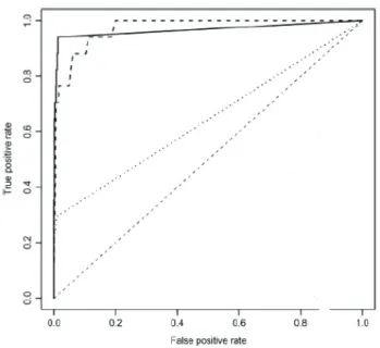
Measuring the goodness of the results of an algorithm is also an important issue. One of the most widely accepted measurement methods in bioinformatics is receiver operat-ing characteristics (ROC) analysis. ROC analysis provides both visual and numerical summary of the classifiers results [9]. Originally developed for radar applications in World War II, it became widely used first in medical applications, later in machine learning and data mining.
Receiver operating analysis is generally used for evaluating the results of a binary classifier. A binary classifier assigns an element to one of two classes, usually noted positive or negative (+ or -). The classification process uses two dis-tinct datasets, the train and the test dataset. In machine learning, the training dataset is used to train the algorithm, in other methods it is used as the basis of calculating the results. Classification methods can be divided further into two distinct categories. Discrete classifiers only predict the classes where the test elements belong. This means, that the classifier can produce 4 different results: true positive, true negative, false positive and false negative. From these, a contingency table can be constructed, and various mea-surements can be counted. Of these, two important ones should be mentioned:
• T P R(true positive rate) = T P T P+F N
• F P R(false positive rate) = F P F P+T N
Where TP, TN, FP, FN denote the four cases mentioned above. The other type of classifiers is the probabilistic clas-sifier. This assigns a value between 0 and 1 to each member of the test set, which can be viewed as a degree of similarity to the distinct classes. This score is then used to create a ranking of elements, and the classifier is good, if the pos-itive elements are at the top of the list. More precisely if we apply a threshold value to this ranking we can create a discrete classifier. By applying multiple threshold values, we can create an infinite number of classifiers.
Using these threshold values we can create a ROC curve by counting the true and false positive rates for each thresh-old value. An example can be seen on Figure 1. Each point of the curve corresponds to a threshold value, which in turn corresponds to a discrete classifier. A ROC curve can be evaluated both numerically and graphically. The ideal
Figure 1: ROC curve
to the unit ramp function. In general, the higher the curve, the better the classification. It must be mentioned, that the curve is only defined between 0 and 1 on each axis. This is of course derived from the fact that both TPR and FPR are values between 0 and 1.
By counting the integral value of the curve we get the “area under curve value”, or AUC. The AUC value of an ideal clas-sifier is 1, the random clasclas-sifier has a value of 0.5. The AUC value can be interpreted as the probability that a randomly chosen positive element is ranked higher than a randomly chosen negative element. In this paper the AUC value in it-self is used to measure the goodness of the results, although it is worth mentioning that a high AUC value does not guar-antee that the positive elements are ranked at the top of the list. This topic is discussed further in [8, 9].
2.3 Propagation algorithms
Originating from graph theory, propagation algorithms re-quire a network containing vertices and edges as the basis of the method. Perhaps the most known propagation method is the PageRank algorithm [6], first used by Google for infor-mation retrieval tasks. Note, that Kleinberg had proposed a very similar algorithm for finding hubs and authorities ear-lier [4].
There are various ranking algorithms specifically for protein classification, namely [1, 2, 5, 10] . In general, these meth-ods use a query mechanism to generate results. With the given similarity network, we add a new element as query, and the classification algorithm calculates the class (or the probability) this element belongs to.
that did not have labels previously. The method described in this paper uses the latter approach, and volunteers to solve the classification task without the need to cut the edges of the similarity network.
3. A SIMPLE PROPAGATION ALGORITHM
The method we propose in this paper is a simple general propagation algorithm for function approximation closely based on the works of [7]. The method is general in a sense, that it was not created solely for the purpose of protein classification, although in this paper we will stick to this example of its application.3.1 The label propagation algorithm by
Ragha-van et al.[7]
Originally a community detection algorithm, the label prop-agation method of Raghavan et al. is based on a simple, but effective idea. In a graph (directed or not) we assign labels to each node. In one iteration step, each nodexadopts the label that a maximum number of its neighborsx1, x2, ..., xk
share. When a tie happens, a random selection is used. At the beginning, each node is initialized with a different label, and as labels propagate through the network, sooner or later a consensus emerges among the densely connected subgraph of the original graph. Communities are formed this way. It is also easy to generalize this method to weighted graphs. An example of this process can be seen on Zachary’s karate club network [11] on Figure 2. The three different shades of grey represent the different labels.
Figure 2: Propagation example
The labels can be updated synchronously or asynchronously. In the first case the labels assigned at iteration number t depend only on the labels of iteration t−1 : Lx(t) = f(Lx1(t−1), Lx2(t−1), ..., Lxk(t−1)), whereL(x) denotes
the label of nodexat iterationt, andf is the update func-tion.
If there are subgraphs in the network, that are bipartite or nearly bipartite in structure this method might oscil-late. The asynchronous update method solves this problem: we consider a node in iteration t. There are some
neigh-the node based on neigh-the labels of neigh-the current iteration in neigh-the case of neighbors, that have already updated their labels. For neighbors not yet updated, we use the labels of itera-tion t−1. Lx(t) =f(Lx1(t), Lx2(t), ..., Lxm(t), Lxm+1(t−
1), Lxm+2(t−1), Lxk(t−1)). In the synchronous case the
order in which we choose the nodes for updating is irrele-vant. In the asynchronous case the order can be important. In the original method a random approach is used.
This algorithm can also be called the coloring algorithm, because the labels can be viewed as colors, and in the end, each community has a different color. The colors or labels can also be viewed as categories, thus if we have only two la-bels, we have two categories, and this correspons to a binary classification problem.
3.2 Application for binary classification
As we have mentioned before, in binary classification the two classes are usually called positive and negative, and there are two distinct datasets used by the algorithm, the train dataset, and the test dataset.A similarity matrix is constructed (according to some com-parison method) between the elements of both datasets. The similarity values are available for the whole dataset, even between the test and train datasets s(x, y) : x, y ∈ (T rain∪T est). If we consider the dataset elements as nodes of a graph, this similarity value defines an edge weight, cre-ating a weighted graph containing both the elements of the train and test datasets.
With a small modification, the algorithm described above can be applied to the protein classification problem. In the original algorithm each node receives an initial label different from all other labels. This is of course not correct for the purpose of binary classification. The labels are only known a priori for the train dataset, so only these nodes get an initial label, and as the algorithm terminates, the unlabeled nodes will get labels as well.
If we apply this algorithm directly to the problem described above, we get very poor results. This is not surprising, since this method (and most community detection methods) are not designed for complete graphs like the similarity networks of this problem.
One obvious way to solve this problem is to convert the graph into an unweighted form by cutting the edges accord-ing to some weight limit, but this results to the also obvious problem of choosing the appropriate value. With luck or af-ter a significant number of trial and error steps, it is possible to get good results. Still, this is not a feasible solution to the problem.
3.3 The AProp method
The method proposed in this paper uses a different ap-proach. Rather than using discrete labels for the algorithm, we work with continuous ones. Theoretically there are no
0 and 1), the algorithm will assign values to the uninitial-ized nodes between these. It is important to point out, that these values should not be thought of as probabilities. They represent some “closeness” to one class or the other. These values can then be evaluated with ROC Analysis to produce a goodness measurement.
The update rules are only shown for the synchronous method. There are two reasons for this. In the original algorithm, the asynchronous update rule was introduced to solve conver-gence issues. These issues occurred because nearly bipartite subgraphs caused fluctuations of the discrete labels. Using continuous labels solves this problem, thus the asynchronous rules are not needed. In contrast to this, just for the sake of curiosity we have implemented the asynchronous version as well, but testing showed that they do not perform as good as the synchronous method.
The labels are updated according to the formula described in the previous section, the only difference being the update function f changing to a simple summation. The label of nodexchanges based on the labels of its neighborsN(x):
Lx(t) = 1
d
y∈N(x)
Ly(t−1),
where ddenotes the degree of x. It is easy to extend this rule for weighted graphs. Letdwdenote the weighted degree
ofx. Lx(t) = 1 dw y∈N(x) s(x, y)Ly(t−1),
where s(x, y) is the similarity value between nodes x and y mentioned above. It is worth noting, that the similarity value is symmetrics(x, y) =s(y, x), so we have designed the algorithm to work with undirected graphs. The initialized labels never change, so they should be left out of the update process. This also reduces time complexity significantly. The algorithm consists of iteration steps, the number of it-erations being a possible parameter. Another way to stop the algorithm would be to count the changes that happen in an iteration, and when this change is below a given min-imum, the algorithm halts. Our experience shows us, that no significant change occurs after 6 to 8 iterations.
The label propagation algorithm of Raghavan et al. begins with initializing each node with a different label. We have dropped this approach because we wanted to use the algo-rithm for binary classification, but since we do not know the labels of the members of the test database a priori, some nodes will be left uninitialized. This leads us to the problem of representing the uninitialized status of nodes.
There are two ways of solving the problem. The first way
of the summation. To do this, first we have to sort out the unlabeled nodes from the neighborhood sets. Also, when we count the weighted degree, we should only consider edges that are incident to labeled nodes. This somewhat changes the update rule.
Lx(t) = 1
ds
y∈Ns(x)
s(x, y)Ly(t−1),
where Ns(x) denotes the sorted neighborhood, and ds
de-notes the sorted degree.
The second method is to assign a value to the uninitialized status. This way, we do not have to change the algorithm at all. But this also leaves us with the question: What value should be used for the uninitialized nodes? This solution is called the “biased” approach. The value of the uninitialized nodes should be chosen accordingly to the two class labels. Depending on these considerations, the algorithm can be further divided into three categories:
• Neutral biased. The value is neutral towards the class labels. For example, the class labels are 0 and 1, the value is 0.5.
• Directly biased. The value is one of the class labels. For example, the class labels are 0 and 1, the value is 0 or 1.
• Indirectly biased. Any value, that is not one of the class labels or the neutral value. In the case of 0 and 1, any value other than 0,1 and 0.5.
In the last two cases, further distinction can be made de-pending on what class label do we choose, or in the third case what class label is closer to the uninitialized value. In the end, there are four (or six) variations of the algorithm. Perhaps it is not a big surprise that these variations perform slightly differently when applied to the protein classification problem.
4. RESULTS
Our method was tested on the SCOP40mini and 3PGK databases [3]. The SCOP40mini database consists of 55 clas-sification tasks, and there are seven similarity (or distance) networks available for it. The 3PGK database consists of ten experiments and four similarity (or distance) networks. Further details of the networks can be seen on [3]. In Tables 2 to 5,
• BLAST stands for the basic local alignment search tool.
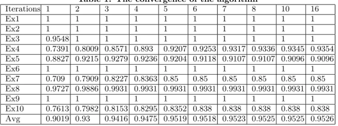
Table 1: The convergence of the algorithm Iterations 1 2 3 4 5 6 7 8 10 16 Ex1 1 1 1 1 1 1 1 1 1 1 Ex2 1 1 1 1 1 1 1 1 1 1 Ex3 0.9548 1 1 1 1 1 1 1 1 1 Ex4 0.7391 0.8009 0.8571 0.893 0.9207 0.9253 0.9317 0.9336 0.9345 0.9354 Ex5 0.8827 0.9215 0.9279 0.9236 0.9204 0.9118 0.9107 0.9107 0.9096 0.9096 Ex6 1 1 1 1 1 1 1 1 1 1 Ex7 0.709 0.7909 0.8227 0.8363 0.85 0.85 0.85 0.85 0.85 0.85 Ex8 0.9727 0.9886 0.9931 0.9931 0.9931 0.9931 0.9931 0.9931 0.9931 0.9931 Ex9 1 1 1 1 1 1 1 1 1 1 Ex10 0.7613 0.7982 0.8153 0.8295 0.8352 0.838 0.838 0.838 0.838 0.838 Avg 0.9019 0.93 0.9416 0.9475 0.9519 0.9518 0.9523 0.9525 0.9525 0.9526
• PRIDE stands for Pride structural similarity.
• LZW stands for the Lempel-Ziv-Welch method.
• DALI stands for DaliLite structural alignment.
• PsiBLAST stands for Position-Specific Iterated BLAST. We have also compared our results with other algorithms provided as a benchmark. Further details of these can be seen on [3]. In Tables 2 to 5,
• 1nn stands for the one nearest neighborhood method.
• RF stands for random forest classification.
• SVM stands for a support vector machine.
• ANN stands for an adaptive neural network.
• LogReg stands for logistic regression.
• AProp stands for approximate propagation.
4.1 Iteration number
For determining the optimal iteration number, we have tested the algorithm on the Smith-Waterman similarity matrix of the 3PGK database. In Table 1, the AUC values are dis-played for the individual experiments and the average value as well.
It can be seen that the values do not change much after it-eration 7, so this was the value we have used for the rest of the evaluation. It is also worth noting that the perfor-mance does not increase monotonously before iteration 7, but fluctuate somewhat.
4.2 3PGK
The results for all variations of the algorithm can be seen in Tables 2 and 3, as well as a comparison against other algorithms. In the first column, the algorithm variations can be seen.
Table 2: Results for 3PGK
Method BLAST SW LA blind 0.9241 0.9470 0.9484 nb 0.9234 0.9412 0.9481 dbn 0.9336 0.9518 0.9473 dbp 0.8973 0.9029 0.9483 idbn 0.9267 0.9317 0.9444 idbp 0.8898 0.9048 0.9485
Table 3: Results for 3PGK
Method BLAST SW LA 1nn 0.8633 0.8605 0.8596 RF 0.8517 0.8659 0.8755 SVM 0.9533 0.9527 0.9549 ANN 0.9584 0.9548 0.9564 LogReg 0.9537 0.9476 0.9593 AProp 0.9336 0.9518 0.9485
• dbp stands for directly biased towards positive.
• idbn stands for indirectly biased towards negative.
• idbp denotes indirectly biased towards positive. If we consider only the variations of the approximation al-gorithm, we can see that none of the approaches appear to be dominant. It can also be seen, that our method performs almost as good as the best approaches.
4.3 SCOP40mini
The results for all variations of the algorithm can be seen in the Tables 4 and 5, as well as a comparison against other algorithms. Unlike in the previous case, the idbp approach outperforms all other variations. We can only guess the rea-son for this behaviour. It is possible, that the experiments in this dataset are structured in a way, that initializing the test dataset towards the positive class label greatly enhances
Table 4: Results for SCOP40mini
Method BLAST SW NW LA PRIDE LZW PsiBLAST DALI
blind 0.899 0.9476 0.9337 0.9442 0.8891 0.8261 0.9083 0.9974 nb 0.9245 0.9492 0.9353 0.9455 0.8897 0.8267 0.9239 0.995 dbn 0.8909 0.9475 0.9335 0.944 0.889 0.826 0.9065 0.9974 dbp 0.932 0.9509 0.9372 0.9466 0.8903 0.8273 0.9304 9977 idbn 0.66 0.9434 0.929 0.9412 0.8876 0.8247 0.7792 0.994 idbp 0.9382 0.9536 0.9405 0.9491 0.8914 0.8283 0.9363 0.998
Table 5: Results for SCOP40mini
Method BLAST SW NW LA PRIDE LZW DALI
1nn 0.7577 0.8154 0.8252 0.7343 0.8644 0.7174 0.9892 RF 0.6965 0.8230 0.8030 0.8344 0.9105 0.7396 0.9941 SVM 0.904 0.9419 0.9376 0.9396 0.9361 0.8288 0.9946 ANN 0.7988 0.8875 0.8834 0.9022 - 0.8346 -LogReg 0.8715 0.9063 0.9175 0.8766 0.9029 0.7487 0.9636 AProp 0.9382 0.9536 0.9405 0.9491 0.8914 0.8283 0.998
It can be seen that our method performs better than the other algorithms in most cases. The running time of the algorithm is very low. The database consists of 55 classi-fication tasks. Solving all of these tasks took 15 minutes on an average notebook computer. This means that for the evaluation of one task, around 16 seconds is needed.
5. CONCLUSION AND FUTURE WORKS
It can be seen from the results, that our algorithm generally performs better on larger databases, with the running time being sufficiently low. The method is relatively general in a way, that it can be used as an approximation algorithm, but it can be extended in several ways described below. This method is very sensitive to the starting labels of the nodes. This can be a weakness, but a proper learning al-gorithm can exploit this property and improve the overall performance of the algorithm.Making the method more general can be difficult. The labeling approach is designed to handle binary classifica-tion tasks. One way to extend this would be to use multi-dimensional labels. Using one number to describe a label corresponds to a one dimensional coordinate. Extending the number of dimensions for the labels would result in multiple classes, while one coordinates would indicate some sort of a membership function towards one class or the other.
Acknowledgment
The author was supported by the Project named “T´ AMOP-4.2.1/B-09/1/KONV-2010-0005 - Creating the Center of Ex-cellence at the University of Szeged” also supported by the European Union and co-financed by the European Regional Fund.
6. REFERENCES
[1] A. B´anhalmi, R. Busa-Fekete, and B. K´egl. A one-class classification approach for protein sequences and structures. InProceedings of the 5th International Symposium on Bioinformatics Research and
Applications, ISBRA ’09, pages 310–322, Berlin, Heidelberg, 2009. Springer-Verlag.
[2] R. Busa-Fekete, A. Kocsor, and S. Pongor. Tree-based algorithms for protein classification. InComputational Intelligence in Bioinformatics, pages 165–182. 2008. [3] http://net.icgeb.org/benchmark/. Protein benchmark
database.
[4] J. M. Kleinberg. Authoritative sources in a hyperlinked environment.J. ACM, 46:604–632, September 1999.
[5] A. Kocsor, R. Busa-Fekete, and S. Pongor. Protein classification based on propagation of unrooted binary trees.Protein and Peptide Letters, 15(5):428–437, June 2008.
[6] L. Page, S. Brin, R. Motwani, and T. Winograd. The pagerank citation ranking: Bringing order to the web. Technical Report 1999-66, Stanford InfoLab,
November 1999. Previous number = SIDL-WP-1999-0120.
[7] U. N. Raghavan, R. Albert, and S. Kumara. Near linear time algorithm to detect community structures in large-scale networks.Phys. Rev. E, 76(3):036106, Sep 2007.
[8] A. K. R´obert Busa-Feketea, Attila Kert´esz-Farkasa and S. Pongor. Balanced roc analysis (baroc) protocol for the evaluation of protein similarities.Journal of Biochemical and Biophysical Methods, 70(6):1210 – 1214, 2008.
[9] P. Sonego, A. Kocsor, and S. Pongor. Roc analysis: applications to the classification of biological sequences and 3d structures.Briefings in Bioinformatics, 9(3):198–209, January 2008. [10] J. Weston, A. Elisseeff, D. Zhou, C. Leslie, and
Optimal and Reliable Covering of
Planar Objects with Circles
Endre Palatinus
Institute of Informatics University of Szeged 2 Árpád tér Szeged, Hungary H-6720[email protected]
ABSTRACT
We developed an algorithm for finding the sparsest cover-ing of planar objects with a given number of circles with fixed centers. The covering is tested reliably using interval arithmetic. We applied our solution to a telecommunication related problem.
Supervisor: Dr. Bal´azs B´anhelyi assistant professor, In-stitute of Informatics, University of Szeged
Categories and Subject Descriptors
G.1.6 [Numerical Analysis]: Optimization—Global opti-mization
1. INTRODUCTION
The circle packing problem has attracted much attention in the last century, and a variant called packings of equal circles in a square receives attention even nowadays [1]. The objec-tive of it is to give the densest packing of a given number of congruent circles with disjoint interiors in a unit square. However, its dual problem, the circle covering has not been exhaustively studied so far. Optimal coverings of the unit square with congruent circles of minimal radii have been found[2] only for small numbers and their optimality have been proved mathematically. Computational methods have been developed[3] to find solutions for higher circle counts, but the produced results were neither computationally reli-able, nor provable approximations of the global optimum. Our aim is to develop a global optimization method for find-ing the sparsest reliable coverfind-ing of a convex or concave pla-nar object with a given number of circles with fixed centers where the sizes of the circles’ radii may be different. By sparsest we mean minimizing the sum of the circles’ area. We have chosen this fitness function, because it can prove useful in many applications, such as covering a region with terrestrial radio signals and determining the optimal energy consumption of wireless sensor networks.
2. RELIABLE COMPUTING
The CPUs of todays personal computers have an arithmetic optimized for computer games. This means that the speed of the computations is more important than the accuracy of them. The floating point computations performed by these CPUs yield results in the domain of the numbers which can be represented in their arithmetic. Since every result is only an approximation of the true results, the error of a complex computation can be arbitrarily large. Consider for example the following expression:
2100+ 2010−2100=?
When calculating the result of this expression using double-precision floating point arithmetic the result will be 0 in-stead of 2010. This is due to the limited precision of the arithmetic.
Mathematicians don’t accept computer assisted proofs if they contain computations performed with unreliable arith-metic. Even the solution of global optimizers can be doubted to be globally optimal ones if we consider that their compu-tations contain accumulated rounding errors. Interval arith-metic is one solution for handling the uncertainty of com-putations. It represents the results of computations as in-tervals, which are guaranteed to contain the precise result. This way it incorporates the rounding errors, too, but does not hide it as the floating point arithmetic does.
3. THE CIRCLE COVERING PROBLEM
Let (r1, r2, . . . , rn) denote the radii of the circles in our con-strained optimization problem. Therefore the fitness func-tion is: f((r1, r2, . . . , rn)) = n i=1 r2 i →min
To solve the previous problem we need:
• a reliable method for testing if a given arrangement is covering or not