in New Energy Aware Scheduling Problems
Thesis submitted in accordance with the requirements of the University of Liverpool for the degree of Doctor in Philosophy by
Hsiang-Hsuan Liu
Notations ix
Preface xi
Abstract xiii
Acknowledgements xv
1 Introduction 1
1.1 Smart Grid Scheduling and Demand Respond Management . . . 1
1.2 Our contribution . . . 3
1.3 Organization of the Thesis . . . 6
2 Preliminaries and Definitions 9 2.1 Offline algorithms and class NP . . . 9
2.1.1 Approximation algorithms . . . 10
2.1.2 Fixed-parameter algorithms . . . 10
2.2 Online algorithms . . . 11
2.3 Scheduling . . . 12
2.4 Smart Grid Scheduling Problem and Definitions . . . 13
3 Literature Review 15 3.1 Previous Work on Smart Grid Scheduling . . . 16
3.1.1 Minimizing peak power demand . . . 16
3.1.2 Minimizing total cost over time . . . 17
3.2 Dynamic Voltage/Speed Scaling Problem . . . 19
3.2.1 Algorithms for theDVS Problem . . . 20
3.2.2 Discrete dynamic voltage/speed scheduling . . . 22
3.2.3 Non-preemptive dynamic voltage/speed scheduling . . . 23
3.3 Related Scheduling Problems . . . 25
3.3.1 Machine minimization . . . 25
3.3.2 Bin Packing problem . . . 27
3.3.3 Load Balancing problem . . . 28
3.4 Related Graph Algorithms . . . 30
3.4.1 Flow problem . . . 30
3.4.2 Matching problem . . . 30 iii
3.5 Summary . . . 33
4 Offline Algorithms for The GRID Problem 35 4.1 NP-hardness . . . 35
4.2 Unit Case . . . 37
4.2.1 Feasibility graph Algorithm . . . 38
4.2.2 Correctness . . . 40
4.2.3 Time Complexity . . . 51
Noncontiguous Feasible Timeslots . . . 51
Contiguous Intervals . . . 52
4.2.4 Using a Discrete DVS Algorithm . . . 55
4.3 Exact Algorithms for Jobs with Arbitrary Widths and Heights . . . 59
4.3.1 Key notions . . . 59
4.3.2 Framework of the algorithms . . . 61
4.3.3 An algorithm with three parameters . . . 67
4.3.4 An algorithm with two parameters . . . 69
4.4 An (36(1 +dlogwmax wmine)(1 +dlog hmax hmine)) α-Approximation Algorithm for General Case . . . 71
4.4.1 Uniform Widths and Uniform Heights Jobs . . . 72
4.4.2 General Input . . . 79
4.5 Summary . . . 85
5 Online Algorithms for The GRID Problem 87 5.1 General Case . . . 90
5.1.1 Unit width and arbitrary height . . . 90
5.1.2 Uniform width and arbitrary height . . . 92
5.1.3 Arbitrary Input . . . 94
5.2 Lower Bound . . . 99
5.3 Special Cases . . . 101
5.3.1 Unit-width and uniform-height . . . 102
5.3.2 Uniform-height, arbitrary widths and agreeable deadlines . . . 103
5.3.3 Uniform height job set with common feasible intervals . . . 106
5.3.4 Unit width job set with common feasible intervals . . . 107
5.4 Summary . . . 109
6 Extensions to Other Problems 111 6.1 Online algorithm: Minimizing the peak power request . . . 111
6.2 The interval graph approach on other problems . . . 116
6.2.1 Minimizing the peak power request . . . 117
6.2.2 Minimizing the total cost with limited power . . . 117
6.3 Summary . . . 118
7 Conclusion 119
List of Figures
1.1 An illustration of demand response management. . . 3
2.1 Illustrations of a job in the GRIDproblem. . . 14
3.1 An illustration of Example 3.1. . . 18
3.2 Illustration of Example 3.2. . . 21
3.3 Illustration of Example 3.4. . . 31
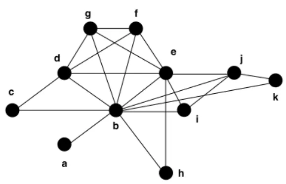
3.4 An input instance and the corresponding interval graph. . . 32
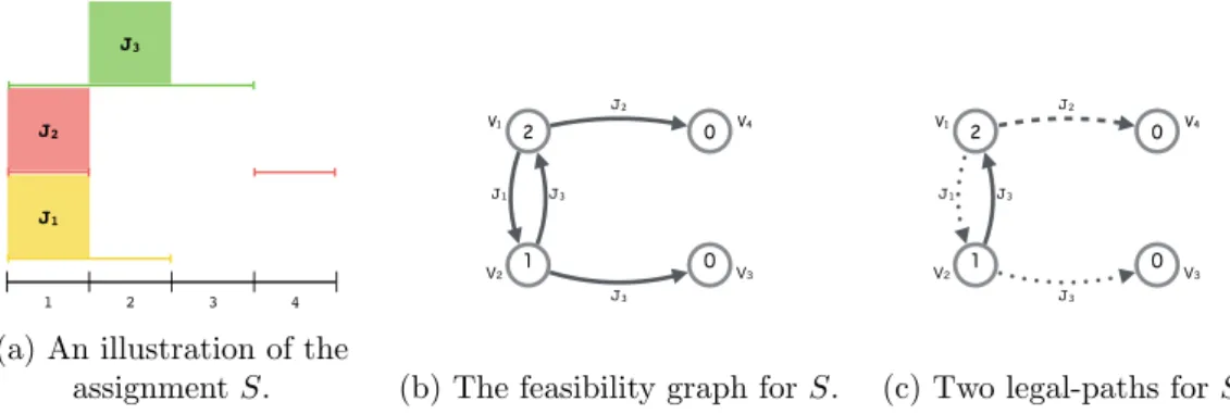
4.1 The feasibility graph and two legal-paths with respect to Example 4.1 . . . . 39
4.2 Example of shifting along a legal-path referring to Example 4.1. . . 39
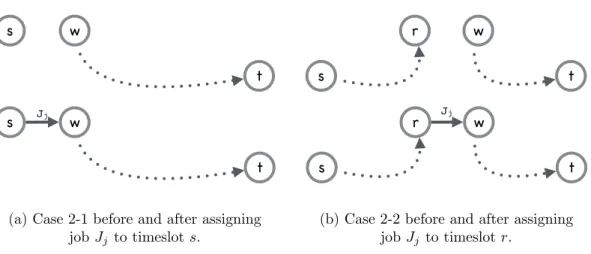
4.3 The two sub-cases of Case 2 in the proof of Lemma 4.5 (the dotted arcs are used to represent paths). . . 43
4.4 IN(r) (green vertices) and OUT(r) (yellow vertices). The three vertices including r with colors green and yellow are in both IN(r) and OUT(r). . . 44
4.5 Illustration of assignments in Example 4.1. . . 48
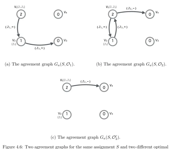
4.6 Two agreement graphs for the same assignmentS and two different optimal schedulesO1 and O2 in Figure 4.5. . . 49
4.7 An illustration of reachable intervals and the path-finder jobs. . . 53
4.8 An illustration of legal path fromstot and the shifting. . . 56
4.9 A set of input jobs and the corresponding interval graph. . . 60
4.10 The windows corresponding to the input in Figure 4.9. . . 61
4.11 ConfigurationsF4(J5). . . 62
4.12 Valid and invalid concatinations ofFleft(J5) and Fright(J5). . . 64
4.13 ConcatinatingFleft(J5) and F4(J5). . . 64
4.14 Illustrations of configurations. . . 65
4.15 Different F4(C4) and the corresponding optimal schedules. . . 66
4.16 An illustration of ProcedureAlignFI. . . 72
4.17 An illustration of Transformation AlignSch. . . 74
4.18 An illustration for Lemma 4.22. . . 76
4.19 An illustration for Lemma 4.25. . . 78
4.20 An illustration for Procedure Convert. . . 80
4.21 An illustration for Lemma 4.29. . . 83
5.1 An illustration for Lemma 4.29. . . 95
5.2 An illustration for Lemma 5.14. . . 96
1.1 Our contribution on minimizing total cost in smart grid . . . 5 3.1 Summarize of results of theDVS problem. . . 24 4.1 Summary of our exact algorithms (n is the number of jobs; wmax is the
maximum width of jobs; m is the maximum size of cliques; Wmax is the
maximum length of windows;k is the number of windows). . . 59
5.1 Summary of our online or approximation algorithms. . . 88
The following notations and abbreviations are found throughout this thesis:
J A set of input jobs J ={J1, J2, J3,· · · }. w(J) Time duration (width) of job J.
h(J) Power request (height) of job J.
I(J) Feasible timeslots ofJ. The set of available timeslots where jobJ can be executed. If I(J) is a contiguous interval, we call it the feasible interval of J.
r(J)The earliest time when job J can be executed.
d(J) The latest time by then jobJ has to be finished.
`oad(S, t) The load at timeslot tin the S schedule.
cost(S) The total cost of the scheduleS.
st(A, J) The start time of job J in theS schedule.
et(A, J)The end time of job J in theS schedule.
DVS The dynamic voltage/speed scaling problem
BINPACKING The bin packing problem
PARTITION The partition problem
AVRThe AVR algorithm of theDVS problem.
BKP The BKP algorithm of the DVS problem.
A significant part of this thesis is based on three peer-reviewed papers that have been published in international conferences and a journal. The four papers have been adapted for the purpose of this thesis and expanded to contain work that was omitted from the conference versions of the papers. The extended versions of the papers are also either under submission for journal publication or in preparation for submission. An additional chapter presents work that has not yet been published that is related to one of the above papers.
Specifically, Sections 4.1 and 4.2 of the thesis are based on the paper entitled “Scheduling for Electricity Cost in Smart Grid”, co-authored with Mihai Burcea, Wing-Kai Hon, Prudence W.H. Wong and David K. Y. Yau. The paper has been published in Proceedings of the 7th Annual International Conference on Combinatorial Optimization and Applications. The journal version is published in the Journal of Scheduling 2016.
Sections 4.3, 4.4 and Chapter 5 of the thesis are based on the paper entitled “Optimal Nonpreemptive Scheduling in a Smart Grid Model”, co-authored with Fu-Hong Liu and Prudence W.H. Wong. The paper has been published in Proceedings of the 27th International Symposium on Algorithms and Computation.
Finally Chapter 6 represents a continuation of the work in Chapters 4 and 5 that focuses on other optimization problems. We show how to solve them by adapting our techniques and prove that our online algorithm can solve the machine minimization problem with an asymptotically optimal competitive ratio. In this chapter we also show that our exact algorithm can be adapt to solve other demand response management problems.
In this thesis, we study the theoretical approach on energy-efficient scheduling problems arising in demand response management in the modern electrical smart grid. Consumers send in power requests with flexible feasible timeslots during which their requests can be served. The grid controller, upon receiving power requests, schedules each request within the specified interval. The electricity cost is measured by a convex function of the load in each timeslot. The objective is to schedule all requests with the minimum total electricity cost.
We study the smart grid scheduling problem in different models. For the offline model, we prove the problem is NP-hard for the general case. We propose a polynomial time algorithm for special input where jobs have unit power request and unit time duration. By adapting the polynomial time algorithm for unit-size jobs, we propose an approximation algorithm for more general input. On the other hand, we also present an exact algorithm to find the optimal schedule for the problem with general input.
For the online model, we propose an online algorithm for jobs with jobs with arbitrary power request, arbitrary time duration, and arbitrary contiguous feasible intervals. We also show a lower bound of the competitive ratio for the smart grid scheduling problem with unit height and arbitrary width. For special cases, we design different online algorithms with better competitive ratios.
Finally, we look at other optimization problems and show how to solve them by adapting our techniques. We prove that our online algorithm can solve the machine minimization problem with an asymptotically optimal competitive ratio. We also show that our exact algorithm can be adapted to solve other demand response management problems.
This project is a long journey. This journey would not be completed without the help of people around me. In this small section of acknowledgments, I would like to use this opportunity to show my gratitude.
I would like to express my immense gratitude to my supervisor, Prudence W.H. Wong. It is my pleasure of working with her. She has widened my view and shown me the beauty of problem-solving, critical thinking, and conciseness. This thesis would not have been possible without her wise mentorship and guidance. I am also grateful for Prudence’s kind help and suggestions in many things throughout these years.
I also want to thank my supervisor in NTHU, Wing-Kai Hon, for his great support. Under his guidance and encouragement I can pursue many different research topics which I am interested in.
A great aid in evaluating my progress throughout the years was provided by my advisors, Paul Spirakis and Michele Zito. I am very greatfull for their suggestions on improving and expanding the work in this thesis.
Furthermore, I want to thank Ton Kloks, with whom I started the systematic re-search. Through him I can take a glimpse at how a decent researcher would be. I also want to thank my collaborators for material in this thesis, Mihai Burcea, Fu-Hong Liu, and David K. Y. Yau. I enjoyed the discussion with them very much and learned a lot from them.
I would like to thank my examiners, George Mertzios and Paul Spirakis. I am very grateful for their thoroughness and advice in revising this thesis to its final version.
Finally, I am going to thank Fu-Hong Liu for his constant support, encouragement, and unconditional love. To me, he is the light in the darkest time.
Introduction
This thesis is a theoretical study on energy-efficient scheduling problems arising in “de-mand response management” in the modern electrical smart grid [25, 33, 38, 59, 84]. The electrical smart grid is one of the major challenges in the 21st century [23, 78, 79]. The smart grid [26, 62] is a power grid system that makes power generation, distribution, and consumption more efficient through information and communication technologies against the traditional power system. By the ability of communication, the smart grid management system is able to provide advanced management, improve energy efficiency and reduce cost [25].
There are many important issues in the research on smart grid [25]. For instance, the infrastructure of smart grid in which the energy can be monitored, the communication technology, the privacy protection, etc. Also, there are various management objectives like improving energy efficiency, balancing demand and supply, cost reduction, utility maximization, reducing energy consumption, price stabilization, etc.
This thesis focuses on the demand response management [11, 44, 58, 61, 64, 72] of smart grid. We consider the research problem as the following. Consumers send in power requests with a set of flexible feasible time intervals during which their requests can be served. The grid controller, upon receiving power requests, schedules each request within the specified interval. The electricity cost is measured by a convex function of the load in each timeslot. The objective is to schedule all requests with the minimum total electricity cost. We consider both offline and online settings and aim to minimize the total cost in the worst case.
1.1
Smart Grid Scheduling and Demand Respond
Man-agement
Unlike the traditional power grid where the power generator is centralized and the power needs to be transmitted over long distance to users, the smart grid allows distributed generation and uses the bi-directional flow of electricity. By using information and communication technologies in an automated fashion, the smart grid is able to improve
the efficiency and reliability of production and distribution of electricity. The cost of generating electrical power has several factors such as fuel cost, heat rate, waste disposal. Different power sources have different generating cost. Usually the power company will use the cheaper power sources before using the more expensive one. If too many tasks are issued at the same time, the total power demand at the time might exceed the amount which the cheapest power source can supply. Hence a more expensive source have to be employed, and it increases the cost. Research initiatives in the area include [40, 57, 70, 77]. Peak demand hours happen only for a short duration, yet make existing electrical grid less efficient. It has been noted in [12] that in the US power grid, 10% of all generation assets and 25% of distribution infrastructure are required for less than 400 hours per year, roughly 5% of the time [79].
Demand response management. By communicating between producers and con-sumers and making decisions about when and how much the power should be generated, the smart grid can improve the efficiency of electricity generators. According to the information revealed by thedemand profile, which is a curve of demand/electrical load over time, power company can plan how much power they need to generate to satisfy the requests from the consumers at any time. Demand response management is changing the demand profile to match the supply better by shifting requests to different time. It can reduce the peak load and avoid emergency to shift the demands of users from on-peak hours to off-peak hours [11, 44, 58, 61, 64, 72].
The electricity grid supports demand response mechanism and obtains energy effi-ciency by organizing consumption of electricity in response to supply conditions. It is demonstrated in [59] that demand response is of remarkable advantage to consumers, utilities, environment, and society. From the viewpoint of the system operator, effective demand load management brings down the cost of operating the grid, while it reduces electricity prices for users. It is also beneficial for utility providers to keep aggregate power demand as flat as possible since this lowers the cost as well as energy generation and distribution [58]. Considering the whole environment, demand response has the ability to minimize the cost for generating electricity and significantly reduces carbon emissions [59]. Demand response management is not only advantageous to the supplier but also to the consumers as well. It is common that electricity supplier charges accord-ing to the generation cost, i.e., the higher the generation cost the higher the electricity price. Therefore, it is to the consumers’ advantage to reduce electricity consumption at a high price and hence reduce the electricity bill [72].
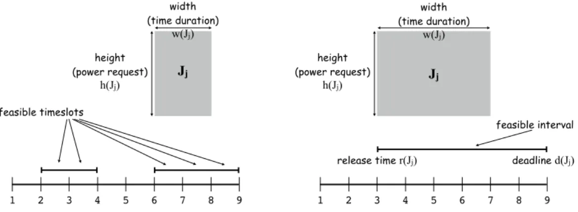
The smart grid operator and consumers communicate through smart metering de-vices [46, 62]. A consumer sends in a power request with the power requirement (cf. height of request), required duration of service (cf. width of request), and the time in-terval that this request can be served (giving some flexibility). For example, a consumer may want the dishwasher to operate for two hours during the periods from 10 a.m. to 12 noon or 2 p.m. to 5 p.m., and the washing machine to operate for one hour during the periods from 9 a.m. to 1 p.m. (see Figure 1.1). The grid operator upon receiving
requests has to schedule them in their respective time intervals using the minimum elec-tricity cost. The load of the grid at each timeslot is the sum of the power requirements of all requests allocated to that timeslot. The electricity cost is modeled by a convex function on the load, in particular, we consider the cost to be the α-th power of the load, where α > 1 is an arbitrary real number. In practice, α is a small constant, e.g.,
α= 2 [21, 73]. 9am 10 11 12
Dishwasher
washing machine
1pm 2 3 4 500 W 1800 W 1 hour 2 hours 5Figure 1.1: An illustration of demand response management.
1.2
Our contribution
Previously, Koutsopoulos and Tassiulas [45] have formulated a similar problem to our problem where the cost is an arbitrary convex function of the load. They claimed that this problem is NP-hard by proving the smart gird scheduling problem with minimizing peak object is NP-hard first, and proposed algorithms to minimize the total cost over the time horizon. For the offline setting, the authors gave an exact algorithm for the preemptive case and claimed that the non-preemptive case is NP-hard. For the online setting, the authors proposed a stochastic model and gave two strategies to minimize the long-term average cost. Their main contribution,Controlled Release strategy, is based on referencing a threshold power level. Given the Poisson distribution of jobs and the cost function, the threshold power level can be decided by running experiments. By deriving a lower bound, the authors proved that as the lengths of feasible intervals increase to infinity, there exists an optimal threshold such that the Controlled Release strategy guarantees asymptotically optimal expectation of total cost under the stochastic model.
Our contribution. We focus on the worst case analysis of the smart grid scheduling problem. Moreover, we consider the case where there is no knowledge of the distribu-tion of release times, deadlines, widths and heights. We first show that this problem is strongly NP-hard, even for very restricted input set or preemptive case. However, we
find that for special input where each job has unit power request and unit time duration, the smart grid scheduling problem can be solved efficiently. We propose a polynomial time offline algorithm that gives an optimal solution and show that the time complex-ity of the algorithm is O(n2τ), where n is the number of jobs and τ is the number of timeslots. We further show that if the feasible timeslots for each job to be served form a contiguous interval, we can improve the time complexity toO(nlogτ+min(n, τ)nlogn). By employing an existing algorithm for the discrete dynamic voltage/speed scaling prob-lem (see Section 3.2.2), we show that the time complexity can be further improved to
O(nlogn).
For more general input set where jobs have arbitrary widths, arbitrary heights, and arbitrary contiguous feasible intervals, we use special graphs to represent the jobs and the important notion maximal cliques to partition the time horizon into disjoint win-dows. The special corresponding intersection graph is an interval graph, which has special properties. These properties direct us to a dynamic programming approach to find the optimal schedule. We propose two exact algorithms; both are fixed-parameter algorithms. By these two fixed-parameter algorithms, we show that the smart grid scheduling problem is fixed-parameter tractable with respect to the maximum width of jobs, and the maximum number of overlapped feasible intervals. That is, when these parameters are constant, the grid problem is no longer NP-hard.
For the general input, we also propose a 36α·(1 +dlogwmax
wmine)
α·(1 +dloghmax
hmine)
α
-approximation algorithm by making use of the optimal scheduling algorithm for unit-size jobs, wherewmax,wmin,hmax, and hmin are the maximum time duration, minimum
time duration, maximum power request, and minimum power request of the input jobs. Comparing with the exact algorithm, the approximation algorithm is more efficient.
For the smart grid problem in online model, we propose the first online algorithm for the general input with worst case competitive ratio, which is polylogarithmic in the max-min ratio of the duration of jobs. Our online algorithms are based on identifying a relationship with the dynamic speed/voltage scaling (DVS) problem. We first propose a 2α(8eα+ 1)-competitive algorithm for jobs with unit time duration and a 12α(8eα+ 1)-compeititve algorithm for jobs with uniform time duration. It means that when α is a constant, both algorithms are constant competitive. By generalizing the result, we present a 36α·(1 +dlogwmax
wmine)
α·(8eα+ 1)-competitive algorithm for general input. The
interesting thing is, our online algorithm and exact algorithms depend on the variation of the job widths but not the variation of the job heights.
On the other hand, we prove that for any deterministic online algorithm, the com-petitive ratio is at least (13logwmax
wmin)
α. The lower bound on the competitive ratio is
proven by an adversary where the input is a set jobs with uniform power request. For special cases of feasible intervals, there are online algorithms which perform better. For jobs with unit time duration, common feasible interval, we propose a 2α-competitive algorithm. For jobs with uniform power request, common release time and common deadline, we propose a 22α-competitive algorithm. For jobs with agreeable deadlines
(which means the jobs released later would have later deadlines) and uniform power request, we prove that a next-fit approach is ((8α2)α + 2α)-competitive. All these online
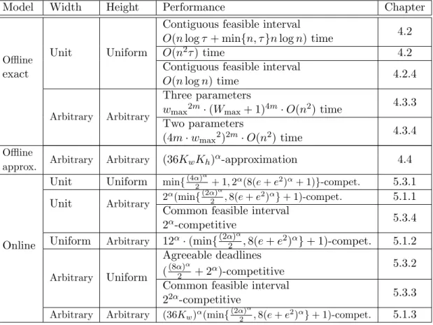
algorithms for special input areO(1)-competitive whenα is a constant. The results are listed in Table 1.1 (Kw is defined as 1 +dwmax
wmine, wherewmaxandwmin are the maximum and minimum widths among all jobs; similarly,Kh is defined as 1 +dhhmaxmine, wherehmax
and hmin are the maximum and minimum heights among all jobs.).
The techniques we use to solve the smart grid scheduling problem are adaptable for other optimization problems. By adapting our online algorithm, we can solve the online machine minimization problem and the peak minimization problem in smart grid optimally in an asymptotic sense. We also elaborate how to use our fixed parameter algorithm to solve the machine minimization problem.
Table 1.1: Our contribution on minimizing total cost in smart grid
Model Width Height Performance Chapter
Offline exact
Unit Uniform
Contiguous feasible interval
O(nlogτ+ min{n, τ}nlogn) time 4.2
O(n2τ) time 4.2
Contiguous feasible interval
O(nlogn) time 4.2.4
Arbitrary Arbitrary
Three parameters
wmax2m·(Wmax+ 1)4m·O(n2) time
4.3.3 Two parameters
(4m·wmax2)2m·O(n2) time 4.3.4 Offline
approx. Arbitrary Arbitrary (36KwKh)
α-approximation 4.4
Online
Unit Uniform min{(4α2)α + 1,2α(8(e+e2)α+ 1)}-compet. 5.3.1
Unit Arbitrary 2
α(min{(2α)α
2 ,8(e+e
2)α}+ 1)-compet. 5.1.1
Common feasible interval
2α-competitive 5.3.4
Uniform Arbitrary 12α·(min{(2α2)α,8(e+e2)α}+ 1)-compet. 5.1.2
Arbitrary Uniform
Agreeable deadlines
((8α2)α + 2α)-competitive 5.3.2
Common feasible interval
22α-competitive 5.3.3
Arbitrary Arbitrary (36Kw)α(min{
(2α)α
2 ,8(e+e
2)α}+ 1)-compet. 5.1.3
The differences between our results and the results in [45]. The main difference is that, in the online model, our goal is to guarantee the worst case performance for the case where and the jobs without knowledge of release times, deadlines, widths, and heights, while in [45], the authors established a stochastic model of the jobs and tried to minimize the longterm average cost. Also, in our work we focus on the cost function which is a power function of the load at any time, whereas in [45] the cost function can be an arbitrary convex function.
For the NP-hardness, the authors in [45] showed it by reducing the bin packing problem to a smart grid problem where jobs have heights and the objective is to minimize
the maximum power consumption over time. By claiming that minimizing the maximum power consumption in the time horizon is equivalent to minimizing the total convex cost in the horizon, the authors claimed that the smart grid problem is NP-hard. Differently, we prove that the smart grid problem is NP-hard by reducing the 3-partition problem directly to the smart grid problem where the objective is to minimize the total cost.
1.3
Organization of the Thesis
The thesis is dedicated to the design and analysis of offline and online algorithms for the smart grid scheduling problem. The work in this thesis is mainly based on the following publications:
1. Mihai Burcea, Wing-Kai Hon, Hsiang-Hsuan Liu, Prudence W. H. Wong, David K. Y. Yau: Scheduling for Electricity Cost in Smart Grid. The 7th Annual Inter-national Conference on Combinatorial Optimization and Applications (COCOA), 2013: 306-317 ([9])
2. Wing-Kai Hon, Hsiang-Hsuan Liu, Prudence W.H. Wong: Online Nonpreemptive Scheduling for Electricity Cost in Smart Grid. The 12th Workshop on Models and Algorithms for Planning and Scheduling Problems (MAPSP), 2015: 193–195 ([35]) 3. Mihai Burcea, Wing-Kai Hon, Hsiang Hsuan Liu, Prudence W. H. Wong, David K. Y. Yau: Scheduling for electricity cost in a smart grid. Journal of Scheduling
19(6): 687-699 (2016) ([10])
4. Fu-Hong Liu, Hsiang-Hsuan Liu, Prudence W.H. Wong: Optimal Nonpreemptive Scheduling in a Smart Grid Model. The 27th International Symposium on Algo-rithms and Computation (ISAAC), 2016: 53:1-53:13 ([54])
Chapter 2 gives preliminaries about algorithms, tractability, and offline/online models. We also mention some commonly used terminologies in scheduling area. We formally define the smart grid scheduling discussed in this thesis.
Chapter 3 looks into a detailed background and history of the smart grid schedul-ing problem. We also elaborate relatschedul-ing schedulschedul-ing problems and algorithms, includschedul-ing dynamic voltage speed/voltage scaling problem (DVS), bin packing problem, machine minimization problem, and load balancing problem. We compare the smart grid schedul-ing problem and these more classical schedulschedul-ing problems; we also make contrast and show the difficulties of adapting the existing solutions. In this chapter, we also discuss graph algorithms and interval graphs, a special graph class. The graph algorithms give us directions to solve the smart grid scheduling problem with special input, and hence we can show that the grid problem with special input is polynomial-time solvable. On the other hand, the special properties of interval graphs give us a way of tickling the gird problem with more general input.
Chapter 4 discusses offline smart grid scheduling problem. First, we prove that the smart grid scheduling problem is NP-hard even when the input is very restricted or preemption is allowed. However, we show that for a special input set with unit-size jobs (that is, each job has unit power request and unit time duration), the optimal schedule can be found in polynomial time. The main idea is using a graph structure to capture all possible assignments of the current input jobs. The results were presented in [9] and the journal version [10]. For the unit-size jobs, we also suggest a faster algorithm by employing the results from the discrete DVS problem (Section 4.2.4.) This result is new and has not published in proceedings. For the smart grid scheduling problem with more general input, we give both approximation algorithms and exact algorithms. A simple approximation algorithm for jobs with unit time duration was presented in [10], and we generalize it to deal with the general input in this thesis (Section 4.4). The approxima-tion algorithms use a classificaapproxima-tion technique and the polynomial time algorithm for the unit-size jobs. On the other hand, the exact algorithms (Section 4.3) are based on the observation of interval graphs. By the exact algorithms, we also prove the smart grid scheduling problem is fixed-parameter tractable with respect to the maximum width of jobs and the maximum number of jobs with overlapped feasible intervals. The results about the exact solution for general input were presented in [54].
Chapter 5 considers the smart grid scheduling problem under the online model. We present an online algorithm for general input with competitive ratio 36α ·(1 + dlogwmax
wmine)
α·(min{(2α)α
2 ,8(e(1 +e))α}+ 1) (Section 5.1). The online algorithm is based
on the one for unit power request input and uniform power request. We also prove that for any deterministic online algorithm, the competitive ratio is at least (α3)α for any constant α and (13logwmax
wmin)
α for arbitrary α. The results were presented in [54].
Furthermore, we investigate online algorithms for special input. We show that when input jobs have restricted width, height, or feasible intervals, there are online strategies with better performance (Section 5.3). The results about online algorithms for special input were presented in [35] and some of the results are further improved in this thesis.
Chapter 6 contains other work which has not been published in proceedings. We show how to use the techniques in this thesis to solve other problems like peak minimiza-tion problem in smart grid model and machine minimizaminimiza-tion problem. We also discuss the smart grid scheduling problem under limited power environment. For the approach to finding an exact solution using interval graphs properties, we investigate some other problems which are able to solve using this framework.
Chapter 7 gives concluding remarks. We also propose future directions for the work.
Preliminaries and Definitions
In this thesis, we mainly investigate the theoretical approach to a smart grid scheduling problem. In the smart grid scheduling problem, each job associates with time duration, power request, and feasible timeslots where it can be executed. The aim is to execute the jobs within their feasible timeslots with the minimum sum of cost at every timeslot, which is convex in the power request at the timeslot. Our aim is to study the smart grid scheduling algorithms which guarantee worst case performance. We consider different models. In the offline model, the algorithms know the whole set of input jobs in advance while in the online model jobs arrive in an online manner and the algorithms have to make decisions without knowledge of the future input.
In this chapter, we give preliminaries about algorithms, tractability, and offline al-gorithms including approximation algorithm and exact algorithm in Section 2.1. In Section 2.2, we give an introduction to online algorithms and competitive analysis. We also introduce some commonly used terminologies in scheduling area in Section 2.3 which is widely used throughout this thesis. In Section 2.4, we formally define the smart grid scheduling problem discussed in this thesis.
2.1
Offline algorithms and class NP
Offline algorithms are algorithms with complete knowledge of the input for the prob-lem in advance. For offline algorithms, one of the measurements of performance of an algorithm is its time complexity. A problem is said to be in class P if it is solvable in polynomial (in the size of the input) time. A problem is in the class NP if any of its yes instance (that is, an instance such that the answer of the decision problem is “yes”) is verifiable in polynomial time. The problems in class P are also in class NP since they are naturally polynomial time verifiable for any yes instance. A problem is NP-hard if all problems in class NP can be reduced to it in polynomial time, even though the problem itself may not be in NP. An NP-hard problem is NP-complete if it is in NP.
There are many problems that have been proved to be in class NP. Some very clas-sical ones are partition problem, bin packing problem, the decision version of traveling salesman problem, the decision version of the 0/1-knapsack problem, etc. [30]. Most of
the optimization problems, including the smart grid scheduling problem, are NP-hard. We introduce the partition problem and bin packing problem:
The PARTITION problem. Given a set of integersA={a1, a2,· · · , an}, decide if
there exists a subset ofA such that the sum of integers in the subset is equal to half of the summation of all integers.
TheBINPACKINGproblem. Given a set of itemsA={a1, a2,· · · , an}and infinite
supply of bins each with capacityc, decided if there exists a number ofB bins to pack the items such that the total size of the items in a bin does not exceed the bin capacity. A problem might have numerical parameters. For example, the magnitudes of the integers in the input to thePARTITIONproblem and the size of items and the capacity of bins in theBINPACKINGproblem. The numerical parameters are part of the input to the problem. For any NP-complete problem, there is no polynomial (in the input size) time algorithm unless P=NP. If there exists an algorithm for the NP-hard/complete problem whose running time is pseudo-polynomial in the input, the problem is said to beweakly NP-hard/complete(NP-hard/complete in the weak sense). On the other hand, a problem isstrongly NP-hard/complete (NP-hard/complete in the strong sense), if it remains NP-hard/complete even when all the numerical parameters are polynomial in the input size. The BINPACKING problem is strongly NP-complete, while the PARTITION problem is weakly NP-complete.
2.1.1 Approximation algorithms
To solve NP-complete or NP-hard problems efficiently, the optimality might be sacri-ficed. In other words, there are trade-offs between the optimality and the efficiency. An algorithm which can find nearly optimal solutions within polynomial time may be good enough. Approximation algorithms are offline algorithms finding nearly optimal solutions.
We use approximation ratio to measure the performance of approximation algo-rithms. The approximation ratio of an algorithm is the worst case of its cost divided by the optimal cost for all feasible input. Consider a minimization problem and let A be an approximation algorithm. We denote A(I) as the cost of the output of algo-rithmA with inputI. We say thatAisc-approximate if for any legal input I, we have cost(A(I))≤c·cost(O(I)) +b, whereO is the optimal solution andb is a non-negative constant.
2.1.2 Fixed-parameter algorithms
Exact algorithms seek an optimal solution for optimization problems. The running time of these algorithms could be very large, especially for NP-hard problems. It is unknown if an NP-complete problem can be solved in polynomial time in the input size of the problem. In parameterized complexity theory, the complexity of a problem is not only
measured regarding the input size, but also in terms of parameters. Generally speaking, an algorithm is afixed-parameter algorithm if it solves a problem with input sizen and a set of parameters {p1, p2,· · · } inf(p1, p2,· · ·)·O(g(n)) time for some function f and
some polynomial function g.
A problem isfixed-parameter tractable if it admits a fixed-parameter algorithm. The idea is that, by restricting parameters which are allowed to have exponential growth running time, we may get knowledge of how these parameters or characters of the prob-lem influence the complexity. Hence, by studying fixed-parameter algorithms we might know better about which parameters make the decision-making so difficult. On the other hand, the parameters might be assumed to be small, and the time complexity of the fixed-parameter algorithm would be small if the parameters are small. That is, we can claim that if the parameters are small, the problem can be solved efficiently.
For a problem, there might be many different sets of parameters. Different ways of parameterizing a problem give different insights into the complexity of the problem, and there is no parameterization which is better than others. For example, in the
CNF-SATISFIABILITYproblem, some possible parameters are clause size, the number of variables, the number of clauses, etc. [66].
2.2
Online algorithms
In online computation, an algorithm has to make decisions based on past events and without information about future. Once a decision is made, it cannot be changed. Such algorithms are called theonline algorithms. The difficulty of designing online algorithms is that each decision is made without knowing the whole picture of the input, and the impact of each decision influences the cost or performance of the final solution. In Section 5, we consider online algorithms, where the job information is only revealed at the time the job is released; the algorithm has to decide which jobs to run at the current time without future information and decisions made cannot be changed later.
There are two types of online models, online time model and online list model. In the online time model, the information of each job is known at the time it is available. Hence the available time of a job is equal to its release time and the job released earlier would be available earlier. In the online list model, the jobs are released according to an ordering. The next job in the ordering will be released once the previously released one is processed. The ordering of releasing does not depend on the earliest time when the jobs are available.
Similarly to the approximation ratio, we usecompetitive ratioto measure the perfor-mance of an online algorithm. The competitive ratio of an algorithm is the worst case of its cost divided by the optimal cost for all feasible input. We letA(I) denote the cost of the output of algorithmAwith inputI. Consider a minimization problem and an online algorithmA. We say thatAisc-competitive if for all feasible input sequenceI, its cost cost(A(I))≤c·cost(O(I)) +b, where O is the optimal solution and b is a constant at
least 0. Notice that O is the optimal offline solution, which knows the whole input in advance. It is worth to mention that any online algorithm is also an approximation and the approximation ratio of the algorithm is exactly its competitive ratio.
The game with adversaries. When analyzing online algorithms, it can be viewed as a game between an online player who runs an online algorithm and an adversary
who can create inputs. In this thesis, we consider adaptive adversaries. An adaptive adversary knows the action of the online player so far, and is able to design the next input according to this knowledge. In the game between an online algorithm and an adversary, the adversary tries to construct the worst possible input for the online algorithm such that the competitive ratio is maximized. In other words, the adversary works to make the competitive ratio as high as possible.
Consider a sequenceIof input generated by an adversary and an online algorithmA. If cost(A(I))≥c·cost(O(I)) for all instanceI, it means that the competitive ratio ofA is at least c. On the other hand, if we can prove that for any online algorithmsA, there is an inputI such that the competitive ratio is at least c, it meanscis the lower bound of the competitive ratio of the optimization problem.
2.3
Scheduling
Scheduling is one of the intensively studied optimization problems. We refer to a survey by Leung [48]. Generally speaking, scheduling is about making decisions to allocate resources to activities with the objective of optimizing one or more measurement of performance. In this thesis, the scheduling problem is to allocate execution timeslots (resources) to jobs (activities) such that the total cost in generating power is minimized.
In the following, we introduce some terminologies widely used in scheduling area.
Preemptive and non-preemptive scheduling. In preemptive scheduling, jobs are allowed to stop temporarily and resume later. On the other hand, innon-preemptive
scheduling, once a job starts executing, the execution will not stop until the task is finished. In this thesis, we consider non-preemptive scheduling.
The earliest deadline first (EDF) principle. The EDF principle is a natural strategy of scheduling. It defines the ordering of job executions according to their deadlines. At any time, the EDF principle chooses the job with the minimum deadline to be executed.
Special inputs. There are some special inputs discussed in scheduling problems. A clique instance is a set of jobs all containing at least one common timeslot. That is, a clique instance is a set of jobsJ1, J2,· · ·, with at least one timeslott∈I(Ji) for all i,
whereI(Ji) is the feasible interval of job Ji.
The jobs with agreeable deadlines means that for any two jobs J1 and J2, if J1 is
More formally, for any two jobsJ1 andJ2 with their own feasible intervals [r(J1), d(J1))
and [r(J2), d(J2)), respectively, r(J1)≤r(J2) implies d(J1)≤d(J2).
A laminar instance is another well-know special input set. In laminar case, any two jobs J1 and J2 are either disjoint or one’s feasible interval is completely inside the the
other’s feasible interval. That is, either [r(J1), d(J1))∩[r(J2), d(J2)) =∅, [r(J1), d(J1))⊆
[r(J2), d(J2)), or [r(J1), d(J1))⊇[r(J2), d(J2)).
2.4
Smart Grid Scheduling Problem and Definitions
In this thesis, we consider a smart grid scheduling problem. The input to the smart grid scheduling problem is a set of jobs with power requests, time durations, and a set of feasible timeslots in which it can be scheduled. The goal is to serve all jobs within their feasible timeslots without preemption such that the total electricity cost is minimized. It can be seen as deciding the time to start each job. According to the schedule, there is a profile of power needs to be generated at each time. That is, the total power request at each timeslot which is determined by the schedule. The cost needed for generating the power is a convex function of the power request at any time [45, 65]. We want to find a schedule such that the total electricity cost of the consequent power profile is as small as possible.
The input. We denote by J = {J1, J2,· · · , Jn} a set of input jobs. Each job Jj
comes withwidthw(Jj),representing the time duration required byJj, andheight h(Jj),
representing the power required by Jj. The work of job Jj, p(Jj), is defined as the product of its power request and its time duration. That is,p(Jj) =w(Jj)×h(Jj). The time is labeled from 1 to τ + 1 and we call the unit time [t, t+ 1) timeslot t. That is, the time is divided into integral timeslotsT ={1,2,3, ..., τ}. Each jobJj also associates with feasible timeslots I(Jj) ⊆ T, representing the set of timeslots when Jj can be executed. We say thatJj isavailable during I(Jj). If the feasible timeslotsI(Jj) of Jj
form a contiguous interval, we call it thefeasible interval ofJj. A feasible intervalI(Jj) is represented by [r(Jj), d(Jj)) where release time r(Jj) is the earliest time Jj can be executed andJj should be finished before itsdeadlined(Jj). We consider events (release
time, deadlines, feasible timeslots) occurring at integral time and assume w(Jj), h(Jj),
r(Jj), andd(Jj), are integers.
Figure 2.1 shows illustrations of jobs. We consider each job Jj as a solid and
unsplit-table rectangle which can be shifted inside its feasible timeslots. An input job set would be a set of this kind of rectangles. Moreover, we assume that the input isfeasible, that is, there exists a schedule such that each of the jobs can be assigned in its feasible timeslots. In other words, for every job Jj, there exist t∈ I(Jj) such that [t, t+w(Jj))⊆I(Jj). The rectangles can be stacked up, which means the corresponding jobs are executed at some same timeslots.
Jj 1 2 3 4 5 6 7 8 9 height (power request) h(Jj) width (time duration) w(Jj) feasible timeslots Jj 1 2 3 4 5 6 7 8 9 height (power request) h(Jj) width (time duration) w(Jj)
release timer(Jj) deadlined(Jj) feasible interval
Figure 2.1: Illustrations of a job in theGRIDproblem.
Feasible schedule. A feasible schedule S has to assign for each job J a start time st(S, J) ∈ I(J) meaning that J runs from [st(S, J), et(S, J)), where for each t ∈ [st(S, J), et(S, J)), t∈I(J). Note that this means preemption is not allowed. Theload
ofS at timet, denoted by`oad(S, t) is the sum of the height (power request) of all jobs running att, i.e.,`oad(S, t) =P
J:t∈[st(S,J),et(S,J))h(J). We dropS and use`oad(t) when
the context is clear. Given an intervalI, the work of a scheduleS within I is defined as
P
t∈I`oad(S, t). For any algorithm A, we use A(J) to denote the schedule of Aon J.
We denote by O the optimal algorithm.
The GRID algorithm. We consider the smart grid scheduling problem where the cost of a scheduleSis the sum of theα-th power of the load over all time, for someα >1, i.e., cost(S) =P
t(`oad(S, t))α. For a set of timeslotsI (not necessarily contiguous), we
denote by cost(S,I) =P
t∈I(`oad(S, t))α. The objective is to find an assignment of all
jobs in J to feasible timeslots such that the total cost is minimized. We call this the
GRIDproblem.
In classical scheduling problems, the objectives usually concern about time. For ex-ample, minimizing flow time is to minimize the sum of the time from releasing a job to the time it is finished; minimizing makespan is to minimize the completion time of the last completed jobs. Unlike the classical scheduling problems, in the smart grid schedul-ing problem, the cost of a certain job dependents on not only its power request and time duration, but also the parameters of the jobs with overlapping execution intervals with it. Because of the convexity of the cost function, it would be much more expen-sive to execute jobs at the same time than to execute jobs without execution timeslots overlapping. In other words, it is better to schedule the jobs evenly over time.
Literature Review
Koutsopoulos and Tassiulas [45] has formulated a similar problem to our problem and the objective is to minimize the long term cost given a distribution of the input jobs. They show that the problem is NP-hard. Feng et al. [27] have claimed that a simple greedy algorithm is 2-competitive for the unit case andα= 2. However, as shown in [55], there is indeed a counter example that the greedy algorithm is at least 3-competitive and so the precise competitiveness of the greedy algorithm is still unknown. This implies that it is still an open question to derive competitive online algorithms for the problem. Salinas et al. [72] considered a multi-objective problem to minimize energy consumption cost and maximize some utility. A closely related problem is to manage the load by changing the price of electricity over time [11, 24, 61, 63]. Heuristics have also been developed for demand side management [58]. Other aspects of smart grid have also been considered, e.g., communication [12, 49, 53, 56], security [56, 60]. Reviews of smart grid can be found in [25, 33, 38, 59, 84].
The combinatorial problem we defined in this thesis has analogy to the traditional load balancing problem [4] and machine minimization problem [13, 16, 17, 71] but the main differences are the objectives. In the load balancing problem, the objective is to minimize the peak load among all machines [4]; in the machine minimization problem, the objective is to minimize the maximum number of machines needed [13, 16, 17, 71]. Minimizing peak load has also been looked at in the context of smart grid [1, 41, 76, 82, 83], some of which further consider allowing reshaping of the jobs [1, 41]. Our problem also has a resemblance to the dynamic speed scaling problem [2, 7, 81] and our algorithms employ some techniques there.
We first review the previous results of the grid problem with the objective to min-imize the peak power request (Section 3.1.1), which has been widely studied. Then we move on to the GRIDproblem, that is, the smart grid scheduling problem with the objective to minimize the total cost (Section 3.1.2), which is the problem we discuss in this thesis. We also elaborate relating scheduling problems and algorithms, including dynamic voltage speed/voltage scaling problem (DVS) (Section 3.2), machine minimiza-tion problem (Secminimiza-tion 3.3.1), bin packing problem (Secminimiza-tion 3.3.2), and load balancing problem (Section 3.3.3). We aim to understand the relation between the GRIDproblem
and these more classical scheduling problems. In this chapter, we also discuss graph algorithms and interval graphs, a special graph class. The graph algorithms give us di-rections to solve the smart grid scheduling problem with special input, and hence we can show that the grid problem with special input is polynomial-time solvable (Section 3.4). On the other hand, the special properties of interval graphs give us a way of tickling the grid problem with more general input (Section 3.4.3).
3.1
Previous Work on Smart Grid Scheduling
In this section, we first review the previous results in the smart grid scheduling problems. Before the research in the grid problem with the objective of minimizing the total cost, the grid problem with the objective of minimizing the peak power request is much widely investigated. We first review the results of the grid problem with the objective of minimizing the peak power request, then move on to the smart grid problem with the objective of minimizing the total cost, which is the problem we discuss in this thesis.
3.1.1 Minimizing peak power demand
The problem of minimizing peak power demand over time has been studied before [68, 69, 76, 82, 83]. The peak minimization problem is similar to theGRID problem but the objective is to find an assignment of all jobs to feasible timeslots such that the peak load along the time is minimized. That is, minimize maxt{`oad(t)}. We call it theGRIDpeak
problem.
Tang et al. [76] studied the GRIDpeakproblem and considered a special case that the
jobs have common feasible interval. That is, each job has same release time and same deadline. They proved that the GRIDpeak problem is NP-hard even for the common
feasible interval special case. They further proposed an offline greedy strategy and proved that it is 7.82-approximate [76, 83].
The authors [76] also discussed another related problem, the Delay Minimization Problem, in which the maximum power supply is given. The Delay Minimization Prob-lem is to schedule the jobs such that the power is no more than the maximum power supply at any time and the objective is to minimize the maximum finish time among all jobs. In other words, if the available power per time unit is limited, how to finish all the requests as soon as possible. For this problem with special input where all jobs have common feasible interval, the online greedy strategy is 2-competitive if there exists a feasible solution.
For the non-preemptive Peak Demand Minimization problem, Yaw et al. [83] further proved that it is even NP-hard to approximate within a factor of 32 −(this holds even for special input where each job has common feasible interval). The proof is by reducing from Bin-Packing problem. The authors proposed a 4-approximation algorithm for the instance where jobs have same release time and same deadline. The basic idea is grouping
jobs by height, splitting the bin recursively, and schedule each group in the different area. For input job set with agreeable deadlines (that is, jobs have later release time must have later deadline), the authors also proposed a O(logwmax
wmin)-approximation algorithm by modifying their algorithm for common feasible interval instance. For general input where jobs have arbitrary release time and arbitrary deadline, the authors proposed a heuristic and experimental results. The heuristic is basically scheduling theless flexible jobs (that is, the jobs with higher d(Jw)(−Jr)(J) ratio) first.
Ranjan et al. [68] studied the preemptive case of theGRIDpeakproblem. They showed
that the GRIDpeak problem is NP-hard even when preemptive is allowed. The authors
further proved that the next-fit decreasing height heuristic is 2-approximate when jobs (with same feasible interval) are all preemptive and 3-approximate when some of the jobs are non-preemptive. In their another paper [69], the authors further improved the approximation ratio upper bound to 1 + 1.7OP T by first-fit decreasing height strategy for instances with both preemptive and non-preemptive jobs.
Yaw et al. [82] investigated an exact algorithm to find an optimal schedule of the non-preemptiveGRIDpeakproblem and gave experimental results. They showed that the
problem is fixed-parameter tractable.
3.1.2 Minimizing total cost over time
In some cases, minimizing peak power demand may not be good enough. Although the peak is minimized, there might be many timeslots with high power demand and hence the total cost is still high. We focus on another objective in the smart grid scheduling problems which is to minimize the total electricity cost. There were some results in minimizing total cost [27, 45, 65]. We first elaborate the relation between the two objectives, minimizing total cost and minimizing peak demand.
Relating to minimizing peak demand. For the same input instance, the ob-jective of minimizing peak or minimizing total cost might leads to different optimal schedule. That is, minimizing the peak demand does not necessarily minimize the to-tal cost, and vice versa. Example 3.1 shows an instance and schedules with respect to minimizing peak and minimizing total cost. The example shows that a schedule with minimized peak may have a higher cost. In other way round, a schedule with minimized cost may have higher peak demand.
Example 3.1. Consider positive integerxandJ ={J1, J2, J3}where w(J1) =w(J2) =
x, h(J1) = h(J2) = 1, w(J3) = 1, h(J3) = 2, I(J1) = I(J2) = [0,2x) and I(J3) =
[x−1, x) (see Figure 3.1a). Figure 3.1b shows a schedule Sc with minimum total cost, which is 3α+ 2x−1. Figure 3.1c shows a schedule Sp with minimum peak, which has
cost (x+ 1)·2α. It is easy to see that the peak in Sc is3, which is higher than the peak in Sp, while the cost in Sc is lower than Sp when x > 3α2−α2−α2−1.
x-1 x 0 2x J2 J3 J1 1 1 1 x x 2
(a) Illustration of the three jobs inJ x-1 x 0 2x J2 J3 J1
(b) ScheduleSc with minimum
total cost x-1 x 0 2x J2 J3 J1
(c) Schedule Sp with minimum
peak Figure 3.1: An illustration of Example 3.1.
Intuitively, when α is big enough, the cost at the peak hour will dominate the total cost. In fact, it was shown in [55] that there is a polynomial time reduction of the decision version of the min-peak problem to that of the min-cost problem for a large enoughα:
Lemma 3.1 ([55]). A grid scheduling problem with objective to minimize the maximum power request can be reduced to a grid scheduling problem with objective to minimize the total cost by settingα >(τ−1)(2P
J∈J h(J) + 1), and the solution of min-cost problem
under this setting is a solution of the corresponding min-max problem.
Previously there were some results in minimizing total cost in smart grid model [27, 45, 65].
Koutsopoulos and Tassiulas [45] studied a similar problem to the GRID problem. Comparing to our problem, their cost function can be an arbitrary convex function while our cost function is anα-power function of load. Moreover, they studied stochastic model and aimed to minimize the expectation of long-term cost while we aim to minimize the total cost and guarantee the worst case performance.
The authors [45] claimed that for instance where jobs can be preempted, the GRID
problem is equivalent to a load balancing problem (and hence NP-hard) and proposed an iterative load balancing algorithm to find an optimal schedule of preemptive jobs. For non-preemptive case of theGRIDproblem, the authors claimed that it is NP-hard.
For the online setting, the authors devised a stochastic model and focused on mini-mizing the long-term average cost. The authors proposed two strategies and proved one of them to be asymptotically optimal by deriving a lower bound for the performance of all policies.
Instead of minimizing the long-term average cost, Feng et al. [27] investigated the worst case competitive ratio of theGRIDproblem under online list setting. In the model time is divided into integral timeslots, each job has unit power request and unit time duration and is released with arbitrary feasible timeslots, which can be non-contiguous. Moreover, the authors consider the case where the cost function is quadratic (that is,
However, Liu et al. [55] proved that greedy strategy is no better than 3-competitive when α = 2 by showing an adversary and hence the precise competitiveness of the greedy algorithm is still unknown.
Narayanaswamy et al. [65] considered a more practical model that other than the power generated by the generator (with quadratic cost function), there is also a renewable resource. The renewable power resource (for example, wind power) varies over time and can only be predicted accurately before short period of time. The generator has to decide how much power to generate such that the generated power together with the renewable power satisfy the time-varying power demand. The objective is to generate sufficient amount of power with minimum regret, which is the difference between the online and the optimal costs. The authors applied recent work in online optimization and proved the algorithm is asymptotically good by deriving bounds in terms of the generator parameters.
Another flourishingly studied problem about optimizing power demand with convex cost function is Dynamic Voltage/Speed Scaling problem. We will discuss in details in Section 3.2
3.2
Dynamic Voltage/Speed Scaling Problem
The combinatorial problem we defined in this thesis has an analogy to the dynamic voltage/speed scaling problem. In this section, we review some famous algorithms for the dynamic voltage/speed scaling problem. In Chapter 5 we will further elaborate how to solve the GRID problem by adapting these algorithms. We also introduce different variations of the dynamic voltage/speed scaling problem and investigate the similarities and differences between these problems and the GRID problem. It gives us fascinating views on how the constraints/properties of the energy-efficient optimization problems affect on the complexities and strategies design.
The theoretical research of dynamic voltage/speed scaling (DVS) problem was raised by Yao, Demers, and Shenker in 1995 [81]. The authors proposed a model of job schedul-ing aimschedul-ing at minimizschedul-ing energy consumption. In their model, job requestsJ are given with their work loads p(J), release times r(J) and deadlines r(J). For each job J, its workp(J) should be finished within [r(J), d(J)) and preemption is allowed. A processor can run at speeds∈[0,∞) and consumes energy in a rate of sα, for some α > 1. The processor with speedsmeans that it can finishsunits of work per unit of time. At any time the scheduler has to decide both which job to be executed and the processor speed to execute the job. The objective is to minimize the total energy consumption. There are different variations of the DVS problem. We also introduce the discrete dynamic
3.2.1 Algorithms for the DVS Problem
In this section, we introduce various algorithms for the DVS problem under offline or online setting.
The YDS algorithm [81]. The authors proposed anO(n2logn) time algorithm for the offline DVS problem wherenis the number of jobs. The key characterization of an optimal schedule is based on the notion ofcritical intervals. A critical interval is a time interval where a group of jobs must be scheduled at maximum, constant speed in any optimal schedule. The offline algorithm is iteratively picking critical intervals by finding intervals having most work has to be done within it. More formally, defineintensity of interval I as the summation of work of jobs with feasible interval completely inside I
divided by the length of |I|, it is easy to see that the intensity of I is a lower bound of the average speed in I. The YDS algorithm iteratively finds the interval I with the highest intensity, assigns the speed as the intensity and runs the jobs completely inside the interval.
It is worth to mention that for the objective minimizing the maximum processor speed, YDS is also optimal [6].
The AVR algorithm [81]. For online DVS problem, Yao et al. [81] proposed the average rate algorithm (AVR). The strategy is based on the density of each job
J, which is defined as d(Jp)(−Jr)(J). In other words, consider an input with a single job, the density of the job is the processor speed in the optimal schedule. At any time t, AVR set the processor speed as the summation of the density of the jobs with feasible interval crossing t and the ordering of jobs execution follows the earliest deadline first (EDF) principle. In other words, in AVR, the schedule and processor speed of each job are considered independently. The final schedule can be seen as stacking up of all independent schedules; at any time, the processor speed is the sum of processor speed in every independent schedule (Figure 3.2c) and the job to be executed is chosen according to the EDF principle (Figure 3.2d). The authors claimed that if the energy consumption function is in the formP(s) =s2, the competitive ratio ofAVRis between 4 to 8. Bansal, Kimbrel, and Pruhs [6] later proved that the AVR algorithm is O(1)-competitive if the energy consumption function is in the formP(s(t)) = (s(t))α.
Lemma 3.2 ([6]). The AVR algorithm is (2α2)α-competitive if the energy consumption function is in the form P(s(t)) = (s(t))α.
Notice thatAVR does not perform well with objective minimizing maximum speed. The following example shows an adversary on whichAVR is Ω(n)-competitive.
Example 3.2. There are n jobs J1, J2,· · · , Jn. For job Jj, its release time r(Jj) = 0,
deadline d(Jj) = 2j−1, and work load `j = 2j−1. The YDS algorithm runs at constant
processor speed 2−21−n all over the time horizon while AVR runs at speed n at time interval [0,1) and speed n−i at time t ∈ [2i−1,2i) for i ≥ 1. The maximum speed of YDS is less than 2 while the maximum speed of AVR is n. Figure 3.2 shows an input set where n= 4.
J2
J3 J1
J4
(a) A input jobs set ofDVS
J2 J3 J1 J4 (b) YDS schedule J2 J3 J1 J4 speed of AVR
(c) How AVR speed is decided
J4J3 J2 J1
speed of AVR
(d) AVR schedule Figure 3.2: Illustration of Example 3.2.
Time complexity of AVR. At any time t, it needs O(n) time to calculate the speed needed at t.
TheBKP algorithm [6]. TheBKP algorithm is proposed by Bansal, Kimbrel, and Pruhs. At time t, BKP considers all possiblewindows with specific proportion before and aftert. More formally, the window, which is a time interval [t1, t2) containingt, must
have the relation that|t2−t1|:|t2−t|=e: 1. TheBKPalgorithm considers all windows
satisfying the property and finds the one with highest average released work load (by timet) completely inside it. That is, let`(t, t1, t2) =Pt≥r(Jj)∧[r(Jj),d(Jj))⊆[t1,t2)`j denote the total work load of jobs which have been released by timetand are completely inside the window [t1, t2). Notice that the window [t1, t2) should satisfy the property stated
above. At any timet,BKP finds the window [t1, t2) which has maximum value of `|(tt,t2−1,tt12|)
and decides the processor speed to be at e× `(t,t1,t2)
|t2−t1| . The ordering of jobs execution follows the earliest deadline first (EDF) principle. The authors proved thatBKP isO (1)-competitive with respective to both total energy consumption and maximum speed:
Lemma 3.3 ([6]). TheBKP algorithm is2(αα−1)αeα-competitive with respect to energy and e-competitive with respect to maximum speed.
If α ≥ 2, the competitive ratio of BKP is at most 8eα. Note that BKP has better competitive ratio than AVR when α ≥ 5. And also, YDS, AVR, and BKP are all independent ofα.
Time complexity of BKP. At any time t, consider the window [t1, t2) with
maximum `(t,t1,t2)
|t2−t1| value, at least one oft1 and t2 is the release time or deadline of some jobs, otherwise `(t,t1,t2)
|t2−t1| is not maximum. Hence the window [t1, t2) can be found in
O(n2
t) time where nt is the number of jobs released by t.
3.2.2 Discrete dynamic voltage/speed scheduling
Unlike theDVSproblem where the speed of the processor can be arbitrary, in the Discrete
DVS problem, the processor speed is restricted to a given set of speeds. In the end of this section, we will see how to related the DVS problems to the GRID problem. The speed restriction of the DiscreteDVSproblem gives us an inspiration: since in theGRID
problem, the power requests of jobs are fixed and not any real value of power request is needed (for example, if all jobs have integral power requests, then the non-integral speeds seem to be redundant), hence, maybe the DiscreteDVS problem is closer to the
GRID problem. In this section we introduce the results of the Discrete DVS problem. In Section 4.2.4, we will show in details how to relate the DiscreteDVS problem to the
GRID problem and elaborate a polynomial time algorithm for the GRID problem with special input by adapting an algorithm for the Discrete DVS problem.
Ishihara and Yasuura addressed the discrete dynamic voltage/speed scheduling prob-lem [39]. In the original (continuous speed) DVS problem, the processor can be run at arbitrary real-valued speed. However, in real world the processor can only run at a speed selected from a given finite set of d speed levels S = {s1, s2,· · ·, sd} where s1 > s2 >· · ·> sd. TheDVS problem with discrete speeds constraint is called discrete
dynamic voltage/speed scheduling problem. Under the discrete speeds constraints, the schedule generated by YDS algorithm may not be valid for the Discrete DVS problem since the processor speed decided by YDS may not be available. Kwon and Kim pro-posed a O(n2logn)-time algorithm (where n is the number of jobs) to find a schedule with optimal energy consumption which also satisfies the discrete speed constraints [47]. The algorithm is based on the YDS algorithm for originalDVS problem, which is prob-ably invalid (for the Discrete DVS problem). If the speed s of YDS schedule in time interval [t1, t2) is not available in the speed setS, the authors transform the YDS
sched-ule to a valid schedsched-ule for the Discrete DVS problem by replacing the speed in [t1, t2)
by si and si+1 (which are both inS) where si > s > si+1.
By directly characterizing the optimal schedule of the Discrete DVS problem, Li et al. [52] proposed an optimal algorithm with running timeO(nlog max{d, n}) wherenis the number of jobs andd is the number of available speeds. The authors also revisited the continuousDVSproblem and improved the running time fromO(n2logn) toO(n2).
Also, the computation lower bound of the discreteDVSproblem is proved to be at least Ω(nlogn) in the algebraic decision tree model.
For the online version of discrete DVS, Li proposed an (2α−(1δ(−α1)(−1)δαα−−1δ()δαα−−11)α + 1)-competitive online algorithm, whereδis the maximum ratio between any pair of adjacent non-zero speed levels [50]. That is,δ = maxsi>0
si
si+1. The algorithm is by transforming AVR to an online heuristic.
3.2.3 Non-preemptive dynamic voltage/speed scheduling
TheDVSproblems we discussed above all allow preemption. One of the main differences between theDVSproblem and theGRIDproblem is that the preemption of jobs is allowed in the DVS problem while the preemption of jobs is not allowed in the GRID problem. It brings up a question: is the GRID problem more related to the non-preemptive DVS
problem than to theDVS problem?
Although the DVSproblem is polynomial time solvable for both single machine and multi-machine [5], the non-preemptive DVS is NP-hard. It can be proved by reducing from the PARTITIONproblem [3]. Moreover, it can be proved to be strongly NP-hard by reducing from the 3-PARTITIONproblem [3]. However, for instance with agreeable deadlines, the non-preemptiveDVS problem is in P [3].
For jobs with equal work loads, the non-preemptiveDVSproblem is polynomial time solvable. Huang and Ott [37] proved it by proposing anO(n4) time algorithm based on dynamic programming.
Bampis et al. [5] proposed a (1+`max
`min)
α-approximation algorithm for the general case,
where `max and `min are maximum work load and minimum work load, respectively.
The algorithm is by transforming the YDS schedule (which is preemptive) to a non-preemptive one. By this result, there is a 2α-approximation algorithm for uniform-workload jobs.
Antoniadis and Huang [3] proposed an approximation algorithm with approximation ratio 25α−4, which is not related to the work loads. This algorithm is based on a 24α−3 -approximation algorithm for laminar case jobs.
In Table 3.1, we summarize the current results of different variations of the DVS
problem under offline or online model.
Relating to theGRIDproblem. DVSandGRIDare both energy-aware scheduling problems. The cost functions in the two problems are in the same convex form. However, the differences between these two problems are crucial and make the design and analysis of algorithms different. One of the main differences is, in the DVS problem, jobs are characterized by work load, which can be finished with any speed (and even different speeds at different time). In contrast, in the GRID problem, the jobs are characterized by fixed power request and time duration, which means each job has to be executed with specific power for a specific duration of time. Not to mention that preemption is allowed

![Table 3.1: Summarize of results of the DVS problem. offline (running time) online (competitve ratio) DVS O(n 2 log n) [52] AVR:2α−1 α α [6] BKP: 2( α−1α ) α e α [6]](https://thumb-us.123doks.com/thumbv2/123dok_us/10216419.2925490/40.893.141.699.151.353/table-summarize-results-problem-offline-running-online-competitve.webp)