How close are the eigenvectors and eigenvalues of the sample and
actual covariance matrices?
Andreas Loukas
´
Ecole Polytechnique F´
ed´
erale Lausanne, Switzerland
February 20, 2017
Abstract
How many samples are sufficient to guarantee that the eigenvectors and eigenvalues of the sample covariance matrix are close to those of the actual covariance matrix? For a wide family of distributions, including distributions with finite second moment and distributions supported in a centered Euclidean ball, we prove that the inner product between eigenvectors of the sample and actual covariance matri-ces decreases proportionally to the respective eigenvalue distance. Our findings implynon-asymptotic
concentration bounds for eigenvectors, eigenspaces, and eigenvalues. They also provide conditions for distinguishing principal components based on a constant number of samples.
1
Introduction
The covariance matrixCof ann-dimensional distribution is an integral part of data analysis, with numerous occurrences in machine learning and signal processing. It is therefore crucial to understand how close it is to the sample covariance, i.e., the matrix Ce estimated from a finite number of samples m. Following
developments in the tools for the concentration of measure, Vershynin showed that a sample size ofm=O(n) is up to iterated logarithmic factors sufficient for all distributions with finite fourth moment supported in a centered Euclidean ball of radius O(√n) [26]. Similar results hold also for sub-exponential distributions [1] and distributions with finite second moment [20].
We take an alternative standpoint and ask if we can do better when only a subset of the spectrum is of interest. Concretely, our objective is to characterize how many samples are sufficient to guarantee that an eigenvector and/or eigenvalue of the sample and actual covariance matrices are, respectively, sufficiently close. Our approach is motivated by the observation that methods that utilize the covariance commonly prioritize the estimation of principal eigenspaces. For instance, in (local) principal component analysis we are usually interested in the first few eigenvectors [9, 18], whereas when reducing the dimension of a distribution one commonly projects it to the span of the first few eigenvectors [16, 12].
Our finding is that the “spectral leaking” occurring in the eigenvector estimation is strongly localized w.r.t. the eigenvalue axis. In other words, the eigenvector eui of the sample covariance is less far likely to lie in the span of an eigenvector uj of the actual covariance when the eigenvalue distance |λi−λj| is large and the concentration of the distribution in the direction ofuj is small. This phenomenon agrees with the intuition that principal components of high variance are easier to estimate, exactly because they are more likely to appear in the samples of the distribution. In addition, it suggests that it might be possible to obtain good estimates of well separated principal eigenspaces from fewer thannsamples.
We provide a mathematical argument confirming this phenomenon. Under fairly general conditions, we prove that m=O k 2 j (λi−λj)2 ! and m=O k 2 i λ2 i ! (1)
samples are asymptotically almost surely (a.a.s). sufficient to guarantee that |heui, uji|and|δλi|/λi, respec-tively, is small for all distributions with finite second moment. Here,kj2 is a measure of the kurtosis of the
10-5 10-3 10-1 101 λj 0 0.2 0.4 0.6 0.8 1 |h ˜ ui , uj i| ˜ u1 ˜ u4 ˜ u20 ˜ u100 hu˜1, u1i (a)m= 10 10-5 10-3 10-1 101 λj 0 0.2 0.4 0.6 0.8 1 |h ˜ ui , uj i| ˜ u1 ˜ u4 ˜ u20 ˜ u100 hu˜4, u4i (b)m= 100 10-5 10-3 10-1 101 λj 0 0.2 0.4 0.6 0.8 1 |h ˜ ui , uj i| ˜ u1 ˜ u4 ˜ u20 ˜ u100 hu˜20, u20i (c)m= 500 10-5 10-3 10-1 101 λj 0 0.2 0.4 0.6 0.8 1 |h ˜ ui , uj i| ˜ u1 ˜ u4 ˜ u20 ˜ u100 hu˜100, u100i (d)m= 1000 Figure 1: Inner productshuei, ujiare localized w.r.t. the eigenvalue axis. The phenomenon is shown for MNIST. Much fewer thann= 784 samples are needed to estimateu1 andu4.
distribution in the direction ofuj. We also attain a high probability bound for distributions supported in a centered and scaled Euclidean ball, and show how our results can be used to characterize the sensitivity of principal component analysis to a limited sample set.
To the best of our knowledge, these are the first non-asymptotic results concerning the eigenvectors of the sample covariance of distributions with finite second moment. Previous studies have intensively investigated the limiting distribution of the eigenvalues of a sample covariance matrix [24, 4], such as the smallest and largest eigenvalues [6] and the eigenvalue support [7]. Eigenvectors and eigenprojections have attracted less attention; the main research thrust entails using tools from the theory of large-dimensional matrices to characterize limiting distributions [3, 13, 22, 5] and it has limited applicability in the non-asymptotic setting where the sample sizem is small andncannot be arbitrary large.
Differently, our arguments follow from a combination of techniques from perturbation analysis and non-asymptotic concentration of measure. Moreover, in contrast to standard perturbation bounds [11, 27] com-monly used to reason about eigenspaces [14, 15], they can be used to characterize weighted linear combinations ofhuei, uji2 overiandj, and they do not depend on the minimal eigenvalue gap separating two eigenspaces but rather on all eigenvalue differences. The latter renders them particularly amendable to situations where the eigenvalue gap is not significant but the eigenvalue magnitudes decrease sufficiently fast.
Our work also connects to subspace methods, where the signal and noise spaces are separated by an appropriate eigenspace projection. In their recent work, Shaghaghi and Vorobyov characterized the first two moments of the projection error, a result which implies sample estimates [23]. Their results are particularly tight, but are restricted to specific projectors and Normal distributions. Finally, we remark that there exist alternative estimators for the spectrum of the covariance with better asymptotic properties [2, 19]. Instead, we here focus on the standard estimates, i.e., the eigenvalues and eigenvectors of the sample covariance.
2
Problem statement and main results
Let x ∈ Cn be a sample of a multivariate distribution and denote by x
1, x2, . . . , xm the m independent samples used to form the sample covariance, defined as
e C= m X p=1 (xp−x¯)(xp−x¯)∗ m , (2)
where ¯x is the sample mean. Denote by ui the eigenvector of C associated with eigenvalue λi, and corre-spondingly for the eigenvectorsuei and eigenvalueseλi ofCe, such that λ1≥λ2≥. . .≥λn. We ask:
Problem 1. How many samples are sufficient to guarantee that the inner product|huei, uji|=|ue
∗
iuj|and the eigenvalue gap |δλi|=|eλi−λi|is smaller than some constant t with probability larger than ?
Clearly, when asking that all eigenvectors and eigenvalues of the sample and actual covariance matrices are close, we will require at least as many samples as needed to ensure thatkCe−Ck2≤t[26]. However, we
might do better when only a subset of the spectrum is of interest. The reason is that inner products|heui, uji| possess strong localized structure along the eigenvalue axis. To illustrate this phenomenon, let us consider the distribution constructed by then= 784 pixel values of digit ‘1’ in the MNIST database. Figure 1, compares the eigenvectors uj of the covariance computed from all 6742 images, to the eigenvectors uei of the sample
covariance matrices Ce computed from a random subset of m = 10, 100, 500, and 1000 samples. For each i= 1,4,20,100, we depict atλj the average of |huei, uji|over 100 sampling draws. We observe that: (i) The magnitude of huei, ujiis inversely proportional to their eigenvalue gap |λi−λj|. (ii) Eigenvectoreuj mostly lies in the span of eigenvectorsuj over which the distribution is concentrated.
We formalize these statements in two steps.
2.1
Perturbation arguments
First, we work in the setting of Hermitian matrices and notice the following inequality:
Theorem 3.2. For Hermitian matrices C and Ce =δC+C, with eigenvectors uj and eui respectively, the
inequality
|huej, uji| ≤
2kδCujk2
|λi−λj|
,
holds for sgn(λi> λj) 2eλi>sgn(λi > λj)(λi+λj)andλi6=λj.
The above stands out from standard eigenspace perturbation results, such as the sin(Θ) Theorem [11] and its variants [14, 15, 27] for three main reasons: First, Theorem 3.2 characterizes the angle betweenany pair of eigenvectors allowing us to jointly bound any linear combination of inner-products. Though this often proves handy (c.f. Section 5), it was not possible using sin(Θ)-type arguments. Second, classical bounds are not appropriate for a probabilistic analysis as they feature ratios of dependent random variables (corresponding to perturbation terms). In the analysis of spectral clustering, this complication was dealt with by assuming that |λi−λj| ≤ |eλi−λj|[15]. We weaken this condition at a cost of a multiplicative factor of 2. In contrast to previous work, we also prove that the condition is met a.a.s. Third, previous bounds are expressed in terms of the minimal eigenvalue gap between eigenvectors lying in the interior and exterior of the subspace of interest. This is a limiting factor in practice as it renders the results only amenable to situations where there is a very large eigenvalue gap separating the subspaces. The proposed result improves upon this by considering every eigenvalue difference.
2.2
Spectral concentration
The second part of our analysis focuses on the covariance and has a statistical flavor. In particular, we give an answer to Problem 1 for various families of distributions.
In the context ofdistributions with finite second moment, we prove in Section 4.1 that:
Theorem 4.1. For any two eigenvectorsuei anduj of the sample and actual covariance respectively, and for
any real number t >0:
P(|heui, uji| ≥t)≤ 1 m 2kj t|λi−λj| 2 , (3)
s.t. the same conditions as Theorem 3.2.
For eigenvalues, we provide the following guarantee:
Theorem 4.2. For any eigenvaluesλi andeλi ofC andCe, respectively, and for anyt >0, we have
P |eλi−λi| λi ≥t ! ≤ 1 m k i λit 2 . Termkj= (E kxx∗u jk22 −λ2
j)1/2captures the tendency of the distribution to fall in the span ofuj: the smaller the tail in the direction of uj the less likely we are going to confuseuei withuj.
Fornormal distributions, we have thatk2
j =λ2j+λjtr(C) and the number of samples needed for|heui, uji|
to be small is m = O(tr(C)/λ2
i) when λj = O(1) and m = O(λi−2) when λj = O(tr(C)−1). Thus for normal distributions, principal componentsuiandujwith min{λi/λj, λi}= Ω(tr(C)1/2) can be distinguished
given a constant number of samples. On the other hand, estimating λi with small relative error requires
m=O(tr(C)/λi) samples and can thus be achieved from very few samples when λi is large1.
In Section 4.2, we also give a sharp bound for the family of distributions supported within a ball (i.e.,
kxk ≤ra.s.).
Theorem 4.3. For sub-gaussian distributions supported within a centered Euclidean ball of radius r, there
exists an absolute constantc, independent of the sample size, such that for any real numbert >0,
P(|huei, uji| ≥t)≤exp 1− c mΦij(t)2 λjkxk 2 Ψ2 ! , (4) whereΦij(t) = |λi−λj|t−2λj 2 (r2/λ
j−1)1/2 −2kxkΨ2 and s.t. the same conditions as Theorem 3.2. Above,kxkΨ
2is the sub-gaussian norm, for which we usually havekxkΨ2 =O(1) [25]. As such, the theorem implies that, wheneverλiλj=O(1), the sample requirement is with high probabilitym=O(r2/λ2i).
These theorems solidify our experimental findings shown in Figure 1. Moreover, combined with the analysis of principal component estimation given in Section 5, they provide a concrete characterization of the relation between the spectrum (eigenvectors and eigenvalues) of the sample and actual covariance matrix as a function of the number of samples, the eigenvalue gap, and the distribution properties.
3
Perturbation arguments
Before focusing on the sample covariance matrix, it helps to studyhuei, ujiin the setting of Hermitian matrices. The presentation of the results is split in three parts. Section 3.1 starts by studying some basic properties of inner products of the form heui, uji, for anyiandj. The results are used in Section 3.2 to provide a first bound on the angle between two eigenvectors, and refined in Section 3.3.
3.1
Basic observations
We start by noticing an exact relation between the angle of a perturbed eigenvector and the actual eigenvectors ofC.
Lemma 3.1. For everyi andj in1,2, . . . , n, the relation (λei−λj) (ue
∗ iuj) =P n `=1(eu ∗ iu`) (u∗jδCu`) holds . Proof. The proof follows from a modification of a standard argument in perturbation theory. We start from the definitionCeeui=eλiuei and write
(C+δC) (ui+δui) = (λi+δλi) (ui+δui). (5) Expanded, the above expression becomes
Cδui+δCui+δCδui=λiδui+δλiui+δλiδui, (6) where we used the fact thatCui=λiuito eliminate two terms. To proceed, we substituteδui=Pnj=1βiju`, where βij =δu∗iu`, into (6) and multiply from the left by u∗j, resulting to:
n X `=1 βiju∗jCu`+u∗jδCui+ n X `=1 βiju∗jδCu`=λi n X `=1 βiju∗ju`+δλiu∗jui+δλi n X `=1 βiju∗ju` (7)
Cancelling the unnecessary terms and rearranging, we have
δλiu∗jui+ (λi+δλi−λj)βik=u∗jδCui+ n
X
`=1
βiju∗jδCu`. (8)
1Though the same cannot be stated about the absolute error|δλ
At this point, we note that (λi+δλi−λj) =eλi−λj and furthermore thatβik=eu∗iuj−u∗iuj. With this in place, equation (8) becomes
δλiu∗jui+ (eλi−λj) (eu ∗ iuj−u∗iuj) =u∗jδCui+ n X `=1 (ue∗iu`)uj∗δCu`−u∗jδCui. (9)
The proof completes by noticing that, in the left hand side, all terms other than (eλi−λj)ue
∗
iuj fall-off, either due tou∗iuj= 0, when i6=k, or becauseδλi=λei−λj, o.w.
As the expression reveals,huei, ujidepends on the orientation ofueiwith respect to all otheru`. Moreover,
the angles between eigenvectors depend not only on the minimal gap between the subspace of interest and its complement space (as in the sin(Θ) theorem), but on every differenceeλi−λj. This is a crucial ingredient to a tight bound, that will be retained throughout our analysis.
3.2
Bounding arbitrary angles
We proceed to decouple the inner products.
Theorem 3.1. For any Hermitian matrices C and Ce =δC+C, with eigenvectors uj and eui respectively,
we have that|eλi−λj| |huei, uji| ≤ kδC ujk2.
Proof. We rewrite Lemma 3.1 as
(eλi−λj)2(eu∗iuj)2= n X `=1 (eu∗iu`) (u∗jδCu`) !2 . (10)
We now use the Cauchy-Schwartz inequality
(eλi−λj)2(ue ∗ iuj)2≤ n X `=1 (ue∗iu`)2 n X `=1 (u∗jδCu`)2= n X `=1 (u∗jδCu`)2=kδC ujk22, (11)
where in the last step we exploited Lemma 3.2. The proof concludes by taking a square root at both sides of the inequality. Lemma 3.2. n P `=1 (u∗jδCu`)2=kδC ujk22.
Proof. We first notice that u∗jδCu`is a scalar and equal to its transpose. Moreover,δC is Hermitian as the difference of two Hermitian matrices. We therefore have that
n X `=1 (u∗jδCu`)2= n X `=1 u∗jδCu`u∗`δCuj =u∗jδC n X `=1
(u`u∗`)δCuj=u∗jδCδCuj=kδCujk22,
matching our claim.
3.3
Refinement
As a last step, we move all perturbation terms to the numerator, at the expense of a multiplicative constant factor.
Theorem 3.2. For Hermitian matrices C and Ce =δC+C, with eigenvectors uj and eui respectively, the
inequality
|huej, uji| ≤
2kδCujk2
|λi−λj|
,
Proof. Adding and subtractingλi from the left side of the expression in Lemma 3.1 gives (δλi+λi−λj) (ue∗iuj) = n X `=1 (ue∗iu`) (u∗jδCu`). (12)
Forλi6=λj, the above expression can be re-written as
|ue∗iuj|= n P `=1 (ue∗iu`) (uj∗δCu`)−δλi(ue ∗ iuj) |λi−λj| ≤2 max n P `=1 (ue∗iu`) (u∗jδCu`) |λi−λj| ,|δλi| |eu ∗ iuj| |λi−λj| . (13)
Let us examine the right-hand side inequality carefully. Obviously, when the condition|λi−λj| ≤2|δλi| is not met, the right clause of (13) is irrelevant. Therefore, for |δλi|<|λi−λj|/2 the bound simplifies to
|eu∗iuj| ≤ 2 n P `=1 (ue∗ iu`) (u∗jδCu`) |λi−λj| . (14)
Similar to the proof of Theorem 3.1, applying the Cauchy-Schwartz inequality we have that
|ue∗iuj| ≤ 2 s n P `=1 (ue∗ iu`)2 n P `=1 (u∗ jδCu`)2 |λi−λj| = 2kδCujk2 |λi−λj| , (15)
where in the last step we used Lemma 3.2. To finish the proof we notice that, due to Theorem 3.2, whenever
|λi−λj| ≤ |eλi−λj|, one has |eu∗iuj| ≤ kδC ujk2 |λei−λj| ≤kδC ujk2 |λi−λj| < 2kδCujk2 |λi−λj| . (16)
Our bound therefore holds for the union of intervals |δλi| <|λi−λj|/2 and |λi−λj| ≤ |λei−λj|, i.e., for
e
λi>(λi+λj)/2 whenλi> λj and foreλi<(λi+λj)/2 whenλi< λj.
4
Spectral concentration
This section builds on the perturbation results of Section 3 to characterize how far any inner productheui, uji and eigenvalue eλi are from the ideal estimates.
Before proceeding, we remark on some simplifications employed in the following. W.l.o.g., we will assume that the mean E[x] is zero and the covariance full rank. Though the case of rank-deficient C is easily handled by substituting the inverse with the Moore-Penrose pseudoinverse, we opt to make the exposition in the simpler setting. In addition, we will assume the perspective of Theorem 3.2, for which the inequality sgn(λi > λj) 2eλi > sgn(λi > λj)(λi +λj) holds. This event occurs a.a.s. when the gap and the sample size are sufficiently large (see Section 4.1.2), but it is convenient to assume that it happens almost surely. Removing this assumption is possible, but is not pursued here as it leads to less elegant and sharp estimates.
4.1
Distributions with finite second moment
Our first flavor of results is based on a variant of the Tchebichef inequality and holds for any distribution with finite second moment.
4.1.1 Concentration of eigenvector angles
We start with the concentration of inner-products|huei, uji|.
Theorem 4.1. For any two eigenvectors uei and uj of the sample and actual covariance respectively, with
λi6=λj, and for any real numbert >0, we have
P(|huei, uji| ≥t)≤ 1 m 2kj t|λi−λj| 2 for sgn(λi> λj) 2eλi >sgn(λi> λj)(λi+λj)andkj= E kxx∗ujk22 −λ2 j 1/2 .
Proof. According to a variant of Tchebichef’s inequality [21], for any random variable X and for any real numbers t >0 andα:
P(|X−α| ≥t)≤Var[X] + (E[X]−α)
2
t2 . (17)
Setting X=huei, ujiandα= 0, we have
P(|huei, uji| ≥t)≤ Var[heui, uji] +E[huei, uji] 2 t2 = Ehuei, uji2 t2 ≤ 4EkδCujk22 t2(λ i−λj)2 , (18)
where the last inequality follows from Theorem 3.2. We continue by expandingδCusing the definition of the eigenvalue decomposition and substituting the expectation.
E kδCujk22 =EhkCue j−λjujk22 i =Ehu∗j(Ce−λj)(Ce−λj)uj i =Ehu∗jCe2uj i +λ2j−2λju∗jE h e Ciuj =Ehu∗jCe2uj i −λ2j. (19) In addition, Ehu∗jCe2uj i = m X p,q=1 u∗j E (xpx∗p)(xqx∗q) m2 uj =X p6=q u∗jE xpx∗p Exqx∗q m2 uj+ m X p=1 u∗jE xpx∗pxpx∗p m2 uj =m(m−1) m2 λ 2 j+ 1 mu ∗ jE[xx ∗xx∗]u j = (1− 1 m)λ 2 j+ 1 mu ∗ jE[xx ∗xx∗]u j (20) and therefore E kδCujk22 = (1− 1 m)λ 2 j+ 1 mu ∗ jE[xx∗xx∗]uj−λ2j =u ∗ jE[xx∗xx∗]uj−λ2j m = E kxx∗ujk22 −λ2 j m .
Putting everything together, the claim follows.
Corollary 4.1. For any weightswij and realt >0: P X i6=j wijhuei, uji2> t ≤ X i6=j 4wijkj2 m t(λi−λj)2 , wherekj = E kxx∗ujk22
−λ2j1/2 andwij 6= 0whenλi6=λj and sgn(λi> λj) 2eλi >sgn(λi> λj)(λi+λj).
Proof. We proceed as in the proof of Theorem 4.1:
P X i6=j wijhuei, uji2 12 > t ≤ EhP i6=jwijhuei, uji 2i t2 ≤ 4 t2 X i6=j wij EkδCujk22 (λi−λj)2 (21)
The claim follows by computingE
kδCujk22
(as before) and squaring both terms within the probability.
4.1.2 Eigenvalue concentration
A slight modification of the same argument can be used to characterize the eigenvalue relative difference.
Theorem 4.2. For any eigenvaluesλi andeλi ofC andCe, respectively, and for anyt >0, we have
P |eλi−λi| λi ≥t ! ≤ 1 m k i λit 2 , whereki= (Ekxx∗uik22 −λi)1/2.
Proof. Directly from the Bauker-Fike theorem [8] one sees that
|δλi| ≤ kCue i−λiuik2=kδCuik2. (22)
The proof is then identical to the one of Theorem 4.1.
As such, the probability the main condition of our Theorems holds is at least
Psgn(λi> λj) 2λei>sgn(λi> λj)(λi+λj) ≥P |eλi−λi|< |λi−λj| 2 >1− 2k 2 i m|λi−λj| . (23)
4.1.3 The influence of the distribution
As seen by the straightforward inequalityE
kxx∗ujk22 ≤E kxk4 2
,kj connects to the kurtosis of the distri-bution. However, it also captures the tendency of the distribution to fall in the span ofuj.
To see this, we will work with the uncorrelated random vectorsε=C−1/2x, which have zero mean and identity covariance. k2j =Ehu∗jC1/2εε∗Cεε∗C1/2uj i −λ2j =λjEu∗jεε ∗Cεε∗u j−λ2j =λj(E h kΛ1/2U∗εε∗ujk22 i −λj). (24)
If we further set ˆε=U∗ε, we have
kj2=λj Xn `=1 λ`E ˆ ε(`)2εˆ(j)2−λj . (25)
It is therefore easier to untangle the spaces spanned byeui andujwhen the variance of the distribution along the latter space is small (the expression is trivially minimized whenλj→0) or when the variance is entirely contained along that space (the expression is also small when λi = 0 for alli 6=j). In addition, it can be seen that distributions with fast decaying tails allow for better principal component identification (E
ˆ
ε(j)4
is a measure of kurtosis over the direction ofuj).
Corollary 4.2. For a Normal distribution, we havek2
j =λj(λj+tr(C)).
Proof. For a centered and normal distribution with identity covariance, the choice of basis is arbitrary and the vector ˆε = U∗ε is also zero mean with identity covariance. Moreover, for every ` 6= j we can write
E ˆ ε(`)2εˆ(j)2 =E ˆ ε(`)2 E ˆ ε(j)2
= 1. This implies that
E kxx∗ujk22 =λ2jE ˆ ε(j)4 +λj n X `6=j λ`=λ2j(3−1) +λjtr(C) = 2λ2j+λjtr(C) (26) and, accordingly, k2 j =λj(λj+ tr(C)).
4.2
Distributions supported in a Euclidean ball
Our last result provides a sharper probability estimate for the family of sub-gaussian distributions supported in a centered Euclidean ball of radius r, with their Ψ2-norm
kxkΨ
2 = sup
y∈Sn−1
khx, yikψ
2, (27)
where Sn−1 is the unit sphere and with theψ
2-norm of a random variable X defined as
kXkψ
2 = sup p≥1
p−1/2E[|X|p]1/p. (28)
Our setting is therefore similar to the one used to study covariance estimation [26]. Due to space constraints, we refer the reader to the excellent review article [25] for an introduction to sub-gaussian distributions as a tool for non-asymptotic analysis of random matrices.
Theorem 4.3. For sub-gaussian distributions supported within a centered Euclidean ball of radius r, there
exists an absolute constantc, independent of the sample size, such that for any real numbert >0,
P(|huei, uji| ≥t)≤exp 1− c mΦij(t)2 λjkxk 2 Ψ2 ! , (29) whereΦij(t) = | λi−λj|t−2λj 2 (r2/λj−1)1/2 −2kxkΨ2,λi6=λj and sgn(λi> λj) 2eλi>sgn(λi > λj)(λi+λj).
Proof. We start from the simple observation that, for every upper boundBof|huei, uji|the relationP(|huei, uji|> t)≤
P(B > t) holds. To proceed therefore we will construct a bound with a known tail. As we saw in Sections 3.3 and 4.1, |huei, uji| ≤ 2kδCujk2 |λi−λj| = 2 (1/m) Pm p=1(xpx∗puj−λjuj) 2 |λi−λj| ≤ 2 Pm p=1 xpx∗puj−λjuj 2 m|λi−λj| = 2Pm p=1 q (u∗ jxp)2(x∗pxp)−2λj(u∗jxp)2+λ2j m|λi−λj| = 2Pm p=1 q (u∗ jxp)2(kxpk22−λj) +λ2j m|λi−λj| (30) Assuming further that kxk2≤r, and since the numerator is minimized when kxpk22 approachesλj, we can write for every sample x=C1/2ε:
q (u∗jx)2(kxk2 2−λj) +λ2j ≤ q (u∗jx)2(r2−λ j) +λ2j =qλj(u∗jε)2(r2−λj) +λ2j ≤ |u ∗ jε| q λjr2−λ2j+λj, (31)
which is a shifted and scaled version of the random variable |εˆ(j)| =|u∗jε|. Setting a= (λjr2−λ2j)1/2, we have P(|huei, uji| ≥t)≤P 2Pm p=1(|εˆp(j)|a+λj) m|λi−λj| ≥t ! =P m X p=1 (|εˆp(j)|a+λj)≥0.5mt|λi−λj| ! =P m X p=1 |εˆp(j)| ≥ m(0.5t|λi−λj| −λj) a ! . (32)
By Lemma 4.1 however, the left hand side is a sum of independent sub-gaussian variables. Since the summands are not centered, we expand each |εˆp(j)| =zp+E[|εˆp(j)|] in terms of a centered sub-gaussian zp with the same ψ2-norm. Furthermore, by Jensen’s inequality and Lemma 4.1
E[|εˆp(j)|]≤E ˆ εp(j)2 1/2 ≤ 2 λj kxkΨ 2. (33) Therefore, if we set Φij(t) = (0.5|λi−λj|t−λj) (r2/λ j−1)1/2 −2kxkΨ2 P(|heui, uji| ≥t)≤P m X p=1 zp≥ mΦij(t) λj ! . (34)
Moreover, by the rotation invariance principle, the left hand side of the last inequality is a sub-gaussian with ψ2-norm smaller than (CP
m p=1kzpk 2 ψ2) 1/2 = (c 1m)1/2kzkψ2 ≤ (Cm/λj) 1/2kxk
Ψ2, for some absolute constant c1. As a consequence, there exists an absolute constantc2, such that for eachθ >0:
P m X p=1 zp ≥θ ! ≤exp 1− c2θ 2λ j mkxk2Ψ 2 ! . (35) Substitutingθ=mΦij(t)/λj, we have P(|huei, uji| ≥t)≤exp 1− c2m2Φij(t)2λj mλ2 jkxk 2 Ψ2 ! = exp 1−c2mΦij(t) 2 λjkxk 2 Ψ2 ! , (36)
which is the desired bound.
Lemma 4.1. If x is a sub-gaussian random vector andε=C−1/2x, then for everyi, the random variable
ˆ
ε(i) =u∗iε is also sub-gaussian, withkεˆ(i)kψ
2 ≤ kxkΨ2/
√
λi.
Proof. The fact that ˆε(i) is sub-gaussian follows easily by the definition of a sub-gaussian random vector, according to which for everyy∈Rn the random variablehx, yiis sub-gaussian. Settingy=ui, the first part is proven. For the bound of the norm, notice that
kxkΨ 2= sup y∈Sn−1 khx, yikψ 2= sup y∈Sn−1 n X j=1 λ1j/2(u∗jy)(u∗jε) ψ 2 ≥ n X j=1 λ1j/2(u∗jui)ˆε(j) ψ 2 =λ1i/2kεˆ(i)kψ 2, (37)
where, for the last inequality, we sety=ui.
5
Principal component estimation
The last step in our exposition entails moving from statements about eigenvector angles to statements about the eigenvectors themselves. In particular, we are going to focus on the eigenvectors of the sample covariance associated to the largest eigenvalues, commonly referred to as principal components.
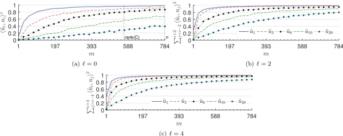
1 197 393 588 784 m 0 0.2 0.4 0.6 0.8 1 h ˜ ui , ui i 2 rank(C) n (a) `= 0 1 197 393 588 784 m 0 0.2 0.4 0.6 0.8 1 Pi + 2 j = i − 2 h ˜ ui , uj i 2 ˜ u1 u˜3 u˜6 u˜10 u˜20 (b)`= 2 1 197 393 588 784 m 0 0.2 0.4 0.6 0.8 1 Pi + 4 j = i − 4 h ˜ ui , uj i 2 ˜ u1 u3˜ ˜u6 u10˜ u20˜ (c)`= 4
Figure 2: Much less thann= 784 samples are needed to estimate principal components associated to large isolated eigenvalues (top). The sample requirement reduces further if we are satisfied by a tight localization of eigenvectors, such that eui is almost entirely contained within the span of the 2`surrounding eigenvectors of ui, shown here for
`= 2 (middle) and`= 4 (bottom).
The phenomenon we will characterize is portrayed in Figure 2. The experiment in question concerns the
n = 784 dimensional distribution constructed by the 6131 images featuring digit ‘3’ found in the MNIST database. The top sub-figure shows the estimation accuracy for a set of five principal components averaged over 200 sampling draws. The trends suggest that the first three eigenvectors can be estimated up to a satisfactory accuracy by much less than n samples. The sample requirements decrease further if we are satisfied by a tight localization of eigenvectors2, such that
e
ui is almost entirely contained within the span of the 2` surrounding eigenvectors of ui. As suggested by the middle and bottom sub-figures, by slightly increasing`, we reduce the number of samples needed to estimate higher principal components.
In the following, we show that our results verify these trends. We are interested to find out how many samples are sufficient to ensure that eui is almost entirely contained within span(ui−`, . . . , ui, . . . , ui+`) for some small non-negative integer `. SettingS={(j < i−`)∪(i+` < j≤r)}, where ris the rank ofC, we have as a consequence of Corollary 4.1 that for distributions with finite second moment:
P i+` X j=i−` huei, uji2<1−t ≤ X j∈S 4kj2 mt(λi−λj)2 (38)
In accordance with the experimental results, equation (38) reveals that it is much easier to estimate the principal components of larger variance, and that, by introducing a small slack in terms of ` one mitigates the requirement for eigenvalue separation.
It might be also interesting to observe that, for covariance matrices that are (approximately) low-rank, we obtain estimates reminiscent of compressed setting [10], in the sense that the sample requirement becomes a function of the non-zero eigenvalues. Though intuitive, this dependency of the estimation accuracy on the rank was not transparent in known results for covariance estimation [20, 1, 26].
6
Conclusions
The main contribution of this paper was the derivation of non-asymptotic bounds for the concentration of inner-products|heui, uji|involving eigenvectors of the sample and actual covariance matrices. We also showed how these results can be extended to reason about eigenvectors, eigenspaces, and eigenvalues.
2This is relevant for instance when we wish to construct projectors over specific principal eigenspaces and we have to ensure
We have identified two interesting directions for further research. The first has to do with obtaining tighter concentration estimates. Especially with regards to our perturbation arguments, we believe that our current bounds on inner products could be sharpened by at least a constant multiplicative factor. We also suspect that a joint analysis of angles could also lead to a significant improvement over Corollary 4.1. The second direction involves using our results for the analysis of methods that utilize the eigenvectors of the covariance for dimensionality reduction. Examples include (fast) principal component projection [12] and regression [17].
References
[1] Rados law Adamczak, Alexander Litvak, Alain Pajor, and Nicole Tomczak-Jaegermann. Quantitative estimates of the convergence of the empirical covariance matrix in log-concave ensembles. Journal of the American Mathematical Society, 23(2):535–561, 2010.
[2] SE Ahmed. Large-sample estimation strategies for eigenvalues of a wishart matrix.Metrika, 47(1):35–45, 1998.
[3] Theodore Wilbur Anderson. Asymptotic theory for principal component analysis. The Annals of Math-ematical Statistics, 34(1):122–148, 1963.
[4] ZD Bai. Methodologies in spectral analysis of large dimensional random matrices, a review. Statistica Sinica, pages 611–662, 1999.
[5] ZD Bai, BQ Miao, GM Pan, et al. On asymptotics of eigenvectors of large sample covariance matrix. The Annals of Probability, 35(4):1532–1572, 2007.
[6] ZD Bai and YQ Yin. Limit of the smallest eigenvalue of a large dimensional sample covariance matrix. The annals of Probability, pages 1275–1294, 1993.
[7] Zhi-Dong Bai and Jack W Silverstein. No eigenvalues outside the support of the limiting spectral distribution of large-dimensional sample covariance matrices. Annals of probability, pages 316–345, 1998.
[8] Friedrich L Bauer and Charles T Fike. Norms and exclusion theorems. Numerische Mathematik, 2(1):137–141, 1960.
[9] Jens Berkmann and Terry Caelli. Computation of surface geometry and segmentation using covariance techniques. IEEE Transactions on Pattern Analysis and Machine Intelligence, 16(11):1114–1116, 1994. [10] Emmanuel J. Cand`es, Xiaodong Li, Yi Ma, and John Wright. Robust principal component analysis?
Journal of the ACM, 58(3):11:1–11:37, June 2011.
[11] Chandler Davis and William Morton Kahan. The rotation of eigenvectors by a perturbation. III. SIAM Journal on Numerical Analysis, 7(1):1–46, 1970.
[12] Roy Frostig, Cameron Musco, Christopher Musco, and Aaron Sidford. Principal component projection without principal component analysis. InProceedings of The 33rd International Conference on Machine Learning, pages 2349–2357, 2016.
[13] V Girko. Strong law for the eigenvalues and eigenvectors of empirical covariance matrices. 1996. [14] Ling Huang, Donghui Yan, Nina Taft, and Michael I Jordan. Spectral clustering with perturbed data.
InAdvances in Neural Information Processing Systems, pages 705–712, 2009.
[15] Blake Hunter and Thomas Strohmer. Performance analysis of spectral clustering on compressed, incom-plete and inaccurate measurements. arXiv preprint arXiv:1011.0997, 2010.
[17] Ian T Jolliffe. A note on the use of principal components in regression. Applied Statistics, pages 300–303, 1982.
[18] Nandakishore Kambhatla and Todd K Leen. Dimension reduction by local principal component analysis. Neural computation, 9(7):1493–1516, 1997.
[19] Xavier Mestre. Improved estimation of eigenvalues and eigenvectors of covariance matrices using their sample estimates. IEEE Transactions on Information Theory, 54(11), 2008.
[20] Mark Rudelson. Random vectors in the isotropic position.Journal of Functional Analysis, 164(1):60–72, 1999.
[21] Dilip Sarwate. Two-sided chebyshev inequality for event not symmetric around the mean? Mathematics Stack Exchange, 2013. URL:http://math.stackexchange.com/q/144675 (version: 2012-05-13).
[22] James R Schott. Asymptotics of eigenprojections of correlation matrices with some applications in principal components analysis. Biometrika, pages 327–337, 1997.
[23] Mahdi Shaghaghi and Sergiy A Vorobyov. Subspace leakage analysis of sample data covariance matrix. InICASSP, pages 3447–3451. IEEE, 2015.
[24] Jack W Silverstein and ZD Bai. On the empirical distribution of eigenvalues of a class of large dimensional random matrices. Journal of Multivariate analysis, 54(2):175–192, 1995.
[25] Roman Vershynin. Introduction to the non-asymptotic analysis of random matrices. arXiv:1011.3027, 2010.
[26] Roman Vershynin. How close is the sample covariance matrix to the actual covariance matrix? Journal of Theoretical Probability, 25(3):655–686, 2012.
[27] Yi Yu, Tengyao Wang, Richard J Samworth, et al. A useful variant of the davis–kahan theorem for statisticians. Biometrika, 102(2):315–323, 2015.