Distributed Bayesian hybrid power state estimation with PMU synchronization errors

(1)

Author(s)

Du, J; Ma, S; Wu, YC; Poor, VH

Citation

The 2014 IEEE Global Communications Conference (GLOBECOM

2014), Austin, TX., 8-12 December 2014. In Conference

Proceedings, 2014, p. 3174-3179

Issued Date

2014

URL

http://hdl.handle.net/10722/214822

(2)

Distributed Bayesian Hybrid Power State Estimation

with PMU Synchronization Errors

Jian Du

∗

, Shaodan Ma

∗

, Yik-Chung Wu

†

and H. Vincent Poor

‡

∗

_{Department of Electrical and Computer Engineering, University of Macau, Macau}

{

jiandu,shaodanma

}

@umac.mo

†

_{Department of Electrical and Electronic Engineering, The University of Hong Kong, Pokfulam Road, Hong Kong}

_{Department of Electrical Engineering, Princeton University, Princeton, New Jersey}

Abstract—This paper presents a distributed hybrid power state estimator, with measurements from both the traditional supervisory control and data acquisition (SCADA) system and the newly invented phasor measurement units (PMUs). The proposed distributed algorithm, which jointly estimates the power states and PMU phase errors, only involves local computations and limited information exchange between neighboring areas, thus alleviating the heavy communication burden compared to the centralized approach. Simulation results show that the performance of the proposed algorithm is very close to that of centralized optimal hybrid state estimates without sampling phase error.

I. INTRODUCTION

Due to the time-varying nature of power generation and consumption, state estimation in the power grid has always been a fundamental function for real-time monitoring of electric power networks [1]. The knowledge of the state vector at each bus, i.e., voltage magnitude and phase angle, enables the energy management system (EMS) to perform various crucial tasks, such as bad data detection, optimizing power flows, maintaining system stability and reliability, etc.

In the past several decades, the supervisory control and data acquisition (SCADA) system has been universally established in the electric power industry, and installed virtually in all EMSs around the world to manage large and complex power systems. In SCADA systems, the voltage magnitude, power injection at each bus and current flow between neighbouring buses are measured and then sent to a master terminal unit to perform state estimation. As these measurements are nonlinear functions of the power states, the state estimation programs are formulated as iterative reweighted least-squares solution [2].

The invention of phasor measurement units (PMUs) [3] has made it possible to measure power states directly, which is infeasible with SCADA systems. Despite the advantage of PMUs over SCADA, the traditional SCADA system cannot be replaced by a PMU-based system overnight. The reason

This work was supported in part by the Macao Science and Technology Development Fund under grant 067/2013/A, in part by the Research Commit-tee of University of Macau under grants MYRG078 and MYRG101, and in part by the U.S. Air Force Office of Scientific Research under MURI Grant FA9550-09-1-0643.

is two fold. Firstly, in practice there are only sporadic PMUs deployed in the power grid due to expensive installation costs. Besides, the SCADA system involves long-term significant investment, and is currently working smoothly in existing power systems. Consequently, hybrid state estimation with both SCADA and PMU measurements is appealing. One straightforward methodology is to simultaneously process both SCADA and PMU raw measurements [4]. However, this simultaneous data processing, which leads to a totally different set of estimation equations, requires significant changes to existing EMS/SCADA systems [5], and is not preferable in practice. In fact, incorporating PMU measurements with minimal change to the SCADA system is an important research problem [5].

In addition to the challenge of integrating PMU with S-CADA data, there are also other practical concerns that need to be considered. Firstly, it is usually assumed that PMUs provide synchronized sampling of voltage and current signals [6] due to the Global Positioning System (GPS) receiver included in the PMU. However, tests [7] provided by a joint effort between the U.S. Department of Energy and the North American Electric Reliability Corporation show that PMUs from multiple vendors can yield up to ±277.8µs sampling phase errors (or ±6◦ phase error in a 60Hz power system) due to different delays in the instrument transformers used by different vendors. Sampling phase mismatch in PMUs will make the state estimation problem nonlinear, which offsets the original motivation for introducing PMUs. It is important to develop state estimation algorithms that are robust to sampling phase errors.

Secondly, with fast sampling rates of PMU devices, a centralized approach, which requires gathering of measure-ments through propagating a significant computational large amounts of data from peripheral nodes to a central processing unit, imposes heavy communication burden across the whole network and imposes a significant computation burden at the control center. Decentralizing the computations across different control areas and fusing information in a hierarchical structure have thus been investigated in [8], [9]. However, these approaches need to meet the requirement of local observ-ability of all the control areas. Consequently, fully distributed

(3)

state estimation scalable with network size is preferred [4], [10]–[12].

In view of above problems, this paper proposes a distributed power state estimation algorithm, which only involves lo-cal computations and information exchanges with immediate neighborhoods, and is suitable for implementation in large-scale power grids. In contrast to [4], [10] and [12], the pro-posed distributed algorithm integrates the data from both the SCADA system and PMUs while keeping the existing SCADA system intact, and the observability problem is bypassed. The challenging problem of sampling phase errors in PMUs is also considered. Simulation results show that after convergence the proposed algorithm performs very close to that of the ideal case which assumes perfect synchronization among PMUs, and centralized information processing.

The following notations are used throughout this paper. Boldface uppercase and lowercase letters will be used for ma-trices and vectors, respectively. _E{·} denotes the expectation of its argument and  _, √−1. Superscript T denotes trans-pose. The symbol IN represents theN×N identity matrix.

N(x|µ,R) stands for the probability density function (pdf) of a Gaussian random vector xwith mean µand covariance matrixR. The symbol∝represents a linear scalar relationship between two real-valued functions. The cardinality of a set V is denoted by |V|and the difference between two sets V and A is denoted byV \ A.

II. HYBRIDESTIMATIONSYSTEMMODEL A. PMU Measurements with Sampling Errors

For a power grid, the continuous voltage on bus i is denoted as Aicos(2πfct+φi), with Ai being the amplitude

and φi being the phase angle in radians. Ideally, a PMU

provides measurements in rectangular coordinates:Aicos(φi)

andAisin(φi). However, for reasons of sampling phase error

[6], [7] and measurement error, the measured voltage at busi

would be [7]

xr_i =Aicos(θi+φi) +wri,E, (1)

x_i =Aisin(θi+φi) +wi,E, (2)

where θi is the phase error induced by an unknown and

random sampling delay, and wr

i,E andw



i,E are the Gaussian

measurement noises. On the other hand, a PMU also measures the current between neighboring buses. Let the admittance at the branch {i, j} be gij+·bij, the shunt admittance at bus

i be Bi, and the transformer turn ratio from bus i to j be

ρij = |ρij|exp{ϕij}. Under sampling phase error, the real

and imaginary parts of the measured current at busiare given by [13]

y_ijr =κ1_ijAicos(θi+φi)−κ2ijAisin(θi+φi)

−κ3_ijAjcos(θi+φj)+κ4ijAjcos(θi+φj)+wi,Ir ,

(3)

y_ij=κ2_ijAicos(θi+φi) +κ1ijAisin(θi+φi)

−κ4_ijAjcos(θi+φj)−κ3ijAjsin(θi+φj) +wi,I,

sinϕ_igij), andwi,I andwi,I are the corresponding Gaussian

measurement errors.

In general, since the phase errorθi is small (e.g., the

max-imum sampling phase error measured by the North American SynchroPhasor Initiative is 6◦ [7]), the standard approxima-tionssinθi≈θi andcosθi ≈1 can be applied to (1) and (2),

leading to [14] x_ir≈E_ir−E_iθi+wi,Er , x  i ≈E  i+E r iθi+w  i,E, (5) whereEr

i ,Aicos(φi)andEi,Aisin(φi)denote the true

power state. Applying the same approximations to (3) and (4) yields y_ijr ≈κ1_ijE_ir−κ2_ijE_i−κ3_ijE_jr+κ4_ijE_j +θi −κ2_ijE_ir−κ1_ijE_i+κ_ij4E_jr+κ3_ijE_j +w_i,Ir , (6) y_ij ≈κ2_ijE_ir+κ1_ijE_i−κ4_ijE_jr−κ3_ijE_j +θi κ1ijEir−κ2ijE  i −κ 3 ijEjr+κ4ijE  j +w  i,I. (7)

We gather all the PMU measurements related to bus i as

zi = [xri, x  i, y r ij1, y  ij1, . . . , y r ijn, y  ijn] T _where _j k is the index

of bus connected to bus i, and arranged in ascending order. Using (5), (6) and (7),zi can be expressed as [14]

zi= X j∈M(i) Hijsj+θi X j∈M(i) Gijsj+wi, (8) where si , [Eir, E 

i]T; M(i) is the set of all immediate

neighboring buses of busi and also includes busi; Hij and

Gij are known matrices containing elements 0, 1 κ1ij, κ2ij,

κ3

ij andκ4ij; and the measurement error vectorwiis assumed

to be Gaussian wi ∼ N(wi|0, σi2I), with σ

2

i being the i th

PMU’s measurement error variance.

B. Mixed Measurement from SCADA and PMUs

For the existing SCADA system, the RTUs measure active and reactive power flows in network branches, bus injec-tions and voltage magnitudes at buses. The measurements of the whole network by the SCADA system can be de-scribed as [5] ζ = g(ξ) + n, where ζ is the vector of the measurements from RTUs in the SCADA system,

ξ _, [A1, φ1, A2, φ2, . . . , A|B|, φ|B|]T with B denoting the

set of buses, and n ∼ N(n|0,W) is the measurement noise from RTUs. Due to the nonlinear function g(·), ξ

can be determined by the iterative reweighted least-squares algorithm [15], and it was shown in [15] that with proper initialization, such a SCADA-based state estimateξˆconverges to the maximum likelihood (ML) solution with covariance matrix Υ = [∇g(ξ)T_W−1_∇_g(ξ)]−1_|

ξ= ˆξ, where ∇g(ξ) is

the partial derivative ofg with respect toξ.

While there are many possible ways of integrating mea-surements from SCADA and PMUs, in this paper, we adopt the approach that keeps the SCADA system intact, as the SCADA system involves long-term investment and is running smoothing in current power networks. In order to incorpo-rate the polar coordinate state estimate ξˆ with the PMU measurements, the work [5] advocates transforming ξˆ into rectangular coordinates, denoted as sˆSCADA , T( ˆξ). Due to

the invariant property of the ML estimator [16], sˆSCADA is

(4)

also the ML estimator in rectangular coordinates. Furthermore, the mean and covariance of sˆSCADA can be approximately

computed using the linearization method [17]. It can be shown that the mean and covariance matrix of sˆSCADA are s and ΓSCADA = ∇T(ξ)Υ∇[T(ξ)]T|ξ= ˆξ, respectively. Since the

goal is to derive a distributed algorithm, it is also assumed that each bus has access only to the mean and variance of its own state from SCADA estimates, i.e.,p(s)≈Qi∈Bp(si) = Q

i∈BN(si|γi,Γi), with γi = [ˆsSCADA]2i−1:2i and Γi =

[PSCADA]2i−1:2i,2i−1:2i. Thus, we have

p(si) =N(si|γi,Γi). (9)

Forp(θ), we adopt the truncated Gaussian model:

p(θi) =T N(θi|θi,θ¯i,v˜i,C˜i) ,[U(θi−θi)−U(θi− ¯ θi)]N(θi|˜vi,C˜i) erf(θ¯i−˜vi ˜ C1_i/2)−erf( θi−v˜i ˜ C_i1/2) , (10)

whereθi andθ¯i are lower and upper bounds of the truncated

Gaussian distribution, respectively; U(x) is the unit step function, whose value is zero for negativexand one for non-negative x; v˜i and C˜i are the mean and covariance of the

original, non-truncated Gaussian distribution; and erf(x) _, 1 √ 2π Rx 0 exp{− y2

2}dy. Moreover, the first order moment of

(10) is ˜ $i=E{θi}=˜vi−C˜ 1/2 i N(¯θi|v˜i,C˜i)− N(θi|v˜i,C˜i) erf(θ¯i−v˜i ˜ C1_i/2)−erf( θi−˜vi ˜ C_i1/2) ,Ξ1[θi,θ¯i,v˜i,C˜i] (11)

and the second order moment is

˜ τi = E{θ2i} = ˜v2_i −2˜viC˜ 1/2 i N(¯θi|˜vi,C˜i)− N(θi|˜vi,C˜i) erf(θ¯i−˜vi ˜ C_i1/2)−erf( θi−v˜i ˜ C_i1/2) + ˜Ci × ( 1−(¯θi−v˜i)N(¯θi|˜vi, ˜ Ci)−(θi−v˜i)N(θi|˜vi,C˜i) ˜ C_i1/2erf(θ¯i−˜vi ˜ C_i1/2)−erf( θi−v˜i ˜ C1_i/2) ) , Ξ2[θi,θ¯i,˜vi,C˜i]. (12)

In general, the parameters of p(θi) can be obtained through

pre-deployment measurements. For example, the truncated range [θi,θ¯i] is founded to be [−6π/180,6π/180]according

to the test results [7]. v˜i and C˜i can also be obtained from

a histogram generated during PMU testing [18]. On the other extreme, (10) also incorporates the case when we have no statistical information about the unknown phase error: setting

[θi,θ¯i] = [−π, π], v˜i = 0, and C˜i =∞, giving an uniform

distributedθi in one sampling period of the PMU.

III. DISTRIBUTEDSTATEESTIMATION UNDERSAMPLING

PHASEERROR

Given all the prior distributions (9), (10) and the likelihood function (8), the MMSE estimator can be written as

ˆ si= 1 c Z . . . Z si Y i∈B p(si) Y i∈P p(θi) ×Y i∈P p(zi|θi,{sj}j∈M(i))d{θi}i∈Pd{s}i∈B, (13) wherec=R . . .R Q i∈Bp(si)Q_i_∈Pp(θi)p(zi|θi,{sj}j∈M(i)) d{θi}i∈Pd{s}i∈B. The integration is complicated as θi is

coupled with{sj}j∈M(i), and its expression is not analytically

tractable. Furthermore, the dimensionality of the state space of the integrand (of the order of number of buses in a power grid, which is typically more than a thousand) prohibits direct numerical integration. In this case, approximate schemes need to be resorted to. One example is the Markov Chain Monte Carlo (MCMC) method, which approximates the distributions and integration operations using a large number of random samples. However, sampling methods can be computationally demanding, often limiting their use to small-scale problems. Even if it can be successfully applied, the solution is centralized, meaning that the network still suffers from heavy communication overhead.

To facilitate the estimation, variational inference is used to approximate the complicated posterior distribution. The goal of variational inference (VI) is to find a tractable variational distributionq(θ,s)that closely approximates the true posterior distribution p(θ,s|z) ∝p(θ)p(s)p(z|θ,s). The criterion for finding the approximatingq(θ,s)is to minimize the Kullback-Leibler (KL) divergence betweenq(θ,s)andp(θ,s|z)[19]:

KL[q(θ,s)||p(θ,s|z)]_,−_Eq(θ,s) lnp(θ,s|z) q(θ,s) . (14)

If there is no constraint onq(θ,s), then the KL divergence vanishes when q(θ,s) = p(θ,s|z). However, in this case, we still face the intractable integration in (13). In the VI framework, a common practice is to apply the mean-field approximation to q(θ,s). For a large-scale power grid, to achieve distributed computation for the power statesi, a

mean-field approximation is applied to q(θ,s), and the variational distribution is in the form q(θ,s) = Q

i∈Pb(θi)Qi∈Bb(si).

Under this mean-field approximation, the optimal b(θi) and

b(si)that minimize (14) are given by (15) and (16) at the top

of the next page. Next, we will evaluate the expressions for

b(θi)andb(si)in (15) and (16), respectively. • Computation ofb(θi):

Assume b(si) is known for all i ∈ B with mean and

covariance denoted by µi and Pi,i, respectively. By

substi-tuting the prior distributions p(si) from (9), p(θi) from (10)

and the likelihood function from (8) into (15), the variational distributionb(θi)can be shown to be

b(θi)∝ T N(θi|θi,θ¯i, vi, Ci) (17) with Ci= ˜ Ci σ_i−2Tr{Bi,2}C˜i+ 1 (18)

(5)

b(θi)∝exp n EQ j∈P\ib(θj)Qi∈Bp(si) lnY i∈P p(zi|θi,{sj}j∈M(i))p(θi) Y i∈B p(si) o i∈ P, ₍₁₅₎ b(si)∝exp n EQ i∈Pb(θi)Qj∈B\ib(sj) Y i∈P p(zi|θi,{sj}j∈M(i))p(θi) Y i∈B p(si) o i∈ B. ₍₁₆₎ vi=Ci ˜ vi/C˜i+σi−2Tr zi X j∈M(i) (Gijµj)T −Bi,1 (19) with Bi,1 = Pj∈M(i)Hij Pj,j + µjµTj GT ij + P j,k∈M(i),j6=kHijµjµ T kGTik andBi,2=P_j_∈M₍_i₎Gij Pj,j +µjµTj GT ij + P j,k∈M(i),j6=kGijµjµTkGTik. With Ci and

vi in (18) and (19), to facilitate the computation ofb(si)in

the next step, the first and second order moments ofb(θi)are

computed through (11) and (12) as

$i= Ξ1[θi,θ¯i, vi, Ci], τi = Ξ2[θi,θ¯i, vi, Ci]. (20)

• Computation ofb(si):

Assume b(θi) for all i ∈ P are known with first and

second order moments denoted by $i and τi, respectively.

Furthermore, it is assumed that b(sj) for j ∈ B \i are also

known with their covariance matrices given by Pj,j. Now,

rewrite (16) as b(si)∝p(si) × Y j∈M(i) expEb(θj)Qk∈M(j)\ib(sk){lnp(zj|θj,{s˜k}˜k∈M(j))} | {z } ,mj→i(si) . (21)

After some matrix multiplications, it can be shown that

mj→i(si)is in Gaussian form mj→i(si)∝ N(si|vj→i,Cj→i) (22) with Cj→i=σ2j[H T jiHji+$j(GTjiHji+HjiTGji)+τjGTjiGji]−1, (23) vj→i=σ−j2Cj→i (Hji+$jGji)Tzj −X k∈M(j)\i H_jiTHjk+$j(GTjiHjk+HjiTGjk)+τjGTjiGjk T µk . (24)

Then, putting p(si) = N(si|γi,Γi) and (22) into (21), we

obtain b(si) ∝ N(si|γi,Γi)N(si|vj→i,Cj→i) ∝ N(si|µi,Pi,i), (25) with Pi,i= (Γ−i 1+ X j∈M(i) C_j−_→1_i)−1 (26) µi=Pi,i(Γ−i1γi+ X j∈M(i) C_j−_→1_ivj→i). (27)

Inspection of (23) and (24) reveals that these expressions can be readily computed at busjand thenCj→iandvj→ican

be sent to its immediate neighbouring bus i for computation of b(si)according to (25).

• Updating Schedule and Summary:

From the expressions forb(θi)andb(si)in (17) and (25),

it should be noticed that these functions are coupled. Conse-quently, b(θi) andb(si) should be iteratively updated. Since

updating any b(θi) or b(si) corresponds to minimizing the

KL divergence in (14), the iterative algorithm is guaranteed to converge monotonically to at least a stationary point [19] and there is no requirement that b(θi)or b(si)should be updated

in any particular order. Besides, the variational distributions

b(θi) and b(si) in (17) and (25) keep the form of truncated

Gaussian and Gaussian distributions during the iterations, thus only their parameters are required to be updated.

However, the successive update scheduling might take too long in large-scale networks. Fortunately, from (23)-(27), it is found that updatingb(si)only involves information within two

hops from bus i. Besides, from (18) and (19), it is observed that updating b(θi) only involves information from direct

neighbours of bus i. Hence, if buses within two hops from each other do not update their variational distributionsb(·)at the same time, the KL divergence in (14) is guaranteed to be decreased in each iteration and the distributed algorithm keeps the monotonic convergence property. This can be achieved by grouping the buses using a distance-2 coloring scheme [20], which colors all the buses under the principle that buses within a two-hop neighborhood are assigned different colors and the number of colors used is the least (for the

IEEE-300 system, only 13 different colors are needed). Then, all buses with the same color update at the same time and buses with different colors are updated in succession. Notice that the complexity order of the distance-2 coloring scheme isQ(λ|B|)

[20], whereλis the maximum number of branches linked to any bus. Sinceλis usually small compared to the network size (e.g.,λ= 9 for the IEEE 118-bus system), the complexity of distance-2 coloring depends only on the network size and it is independent of the specific topology of the power network. In summary, all the buses are first colored by the distance-2

coloring scheme, and the iterative procedure is formally given in Algorithm 1. Notice that although the modelling and formu-lation of state estimation under phase error is complicated, the final result and processing are simple. During each iteration, the first and second order moments of the phase error estimate are computed via (20); while the covariance and mean of the state estimate are computed using (26) and (27). Due to the fact that computing these quantities at one bus depends

(6)

Algorithm 1 Distributed states estimation

1: Initialization: µi = [ˆsSCADA]2i−1:2i and Pi,i =

[PSCADA]2i−1:2i;2i−1:2i.

Neighboring buses exchangeµi andPi,i.

Buses with PMUs update$i andτi via (20).

Every busi computes Ci→j vi→j Pi,i, µi via (23) (24)

(26) (27), and sends these four entities to bus j, where

j∈ M(i).

2: forthelth _iteration_do

3: Select a group of buses with the same color.

4: Buses with PMUs in the group compute$i andτi via

(20).

5: Every bus in the group updates its Ci→j vi→j Pi,i,

µi via (23) (24) (26) (27), and sends them out to its

neighborj.

6: Busj computesvj→kvia (24) and send to its neighbor

k∈ M(j).

7: end for

on information from neighboring buses, these equations are computed iteratively. After convergence, the state estimate is given byµi at each bus.

Although the proposed distributed algorithm advocates each bus to perform computations and message exchanges, but it is also applicable if computations of several buses are executed by a local control center. Then any two control centers only need to exchange the messages for their shared power states.

IV. SIMULATIONRESULTS ANDDISCUSSIONS

This section provides results on the numerical tests of the developed centralized and distributed state estimators in Section III. The network parameters gij, bij, Bi, ρij are

loaded from the test cases in MATPOWER4.0 [21]. In each simulation, the value at each load bus is varied by adding a uniformly distributed random value within ±10% of the value in the test case. Then the power flow program is run to determine the true states. The RTUs measurements are composed of active/reactive power injection, active/reactive power flow, and bus voltage magnitude at each bus, which are also generated from MATPOWER4.0 and perturbed by independent zero-mean Gaussian measurement errors with standard deviation 1×10−2_{. For the SCADA system, the}

estimatesξˆandΥare obtained through the classical iterative reweighted least-squares with initialization[Ai, φi]T = [1,0]T

[13]. In general, the proposed algorithms are applicable re-gardless of the number of PMUs and their placements. But for the simulation study, the placement of PMUs is obtained through the method proposed in [22]. As experiments in [7] show the maximum phase error is 6◦ in a 60Hz power system, θi is generated uniformly from [−6π/180,6π/180]

for each Monte-Carlo simulation run. The PMU measurement errors follow a zero-mean Gaussian distribution with standard deviation σi = 1×10−2. 1000Monte-Carlo simulation runs

are averaged for each point in the figures. Furthermore, it is assumed that bad data from RTUs and PMU measurements has been successfully handled [5], [23, Chap 7].

For comparison, we consider the following three existing methods: 1) Centralized WLS [5] assuming no sampling phase errors in the PMUs. This represents the best performance one can achieve in the state estimation and is a benchmark for the proposed algorithms. 2) Centralized WLS under sampling phase errors in the PMUs. This will show how much degra-dation one would have if phase errors are ignored. 3) The centralized alternating minimization (AM) scheme [14] with

p(s)andp(θi)incorporated as prior information.

Fig. 1 shows the convergence behavior of the proposed algorithms with average mean square error (MSE) defined as ₂_|B|1 P

i∈B||sˆi−si||2. It can be seen that the proposed

distributed algorithm performs close to the optimal perfor-mance after convergence. The seemingly slow convergence is a result of sequential updating of buses with different colors to guarantee convergence. If one iteration is defined as one round of updating of all buses, the distributed algorithm would converge only in a few iterations. On the other hand, part of the degradation from the centralized AM solution is due to the fact that in the distributed algorithm, the covariance of states

si and sj in prior distributions and variational distributions

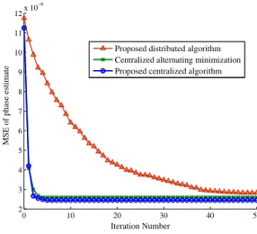
cannot be taken into account. Finally, if the sampling phase error is ignored, we can see that the performance of centralized WLS shows significant degradation, illustrating the importance of simultaneous power state and phase error estimation. Fig. 2 shows the MSE of the sampling phase error estimation

1

|P| P

i∈P||$∗i−θi||2, where$i∗is the converged$i in (20).

It can be seen from the figure that same conclusions as in Fig. 1 can be drawn.

V. CONCLUSIONS

In this paper, a distributed state estimation scheme inte-grating measurements from a traditional SCADA system and newly deployed PMUs has been proposed, with the aim that the existing SCADA system is kept intact, and unknown sam-pling phase errors among PMUs incorporated in the estimation procedure. The proposed distributed power state estimation algorithm only involves limited message exchanges between neighboring buses and is guaranteed to converge. Numerical results have shown that the converged state estimates of the distributed algorithm are very close to those of the optimal centralized estimates assuming no sampling phase error.

REFERENCES

[1] A. Monticelli, “Electric power system state estimation,”Proc. IEEE, vol. 88, no. 2, pp. 262–282, 2000.

[2] G. Giannakis, V. Kekatos, N. Gatsis, S.-J. Kim, H. Zhu, and B. Wollen-berg, “Monitoring and optimization for power grids: A signal processing perspective,” IEEE Signal Process. Mag, vol. 30, no. 5, pp. 107–128, 2013.

[3] A. Phadke, J. Thorp, and M. Adamiak, “A new measurement technique for tracking voltage phasors, local system frequency, and rate of change of frequency,”IEEE Trans. Power App. Syst., vol. PAS-102, no. 5, pp. 1025–1038, 1983.

[4] X. Li and A. Scaglione, “Robust decentralized state estimation and tracking for power systems via network gossiping,”IEEE J. Select. Areas Commun., vol. 31, no. 7, pp. 1184–1194, 2013.

[5] M. Zhou, V. Centeno, J. Thorp, and A. Phadke, “An alternative for including phasor measurements in state estimators,”IEEE Trans. Power Syst., vol. 21, no. 4, pp. 1930–1937, 2006.

[6] A. Phadke and J. Thorp,Synchronized Phasor Measurements and Their Applications. New York: Springer, 2008.

(7)

0 10 20 30 40 50 0 0.1 0.2 0.3 0.4 0.5 0.6 0.7 0.8 0.9 1x 10 Iteration number

MSE of power state estimate

Centralized WLS ignoring non−zero _i

Proposed distributed algorithm Centralized alternating minimization Proposed centralized algorithm Centralized WLS with _i=0

Fig. 1. MSE of the power state versus iteration number for the IEEE118-bus system. 0 10 20 30 40 50 2 3 4 5 6 7 8 9 10 11 12x 10 −6 Iteration Number

MSE of phase estimate

Proposed distributed algorithm Centralized alternating minimization Proposed centralized algorithm

Fig. 2. MSE of the phase error versus iteration number for the IEEE118-bus system.

[7] A. P. Meliopoulos, V. Madani, D. Novosel, G. Cokkinides, andet al., “Synchrophasor measurement accuracy characterization,”North Amer-ican SynchroPhasor Initiative Performance & Standards Task Team (Consortium for Electric Reliability Technology Solutions), 2007. [8] A. Gómez-Expósito, A. Abur, A. de la Villa Jaén, and C. Gómez-Quiles,

“A multilevel state estimation paradigm for smart grids,”Proc. IEEE, vol. 99, no. 6, pp. 952–976, 2011.

[9] R. Ebrahimian and R. Baldick, “State estimation distributed processing for power systems,”IEEE Trans. Power Syst., vol. 15, no. 4, pp. 1240– 1246, 2000.

[10] V. Kekatos and G. Giannakis, “Distributed robust power system state estimation,”IEEE Trans. Power Syst., vol. 28, no. 2, pp. 1617–1626, 2013.

[11] J. Du and Y.-C. Wu, “Distributed clock skew and offset estimation in wireless sensor networks: Asynchronous algorithm and convergence analysis,”IEEE Trans. Wireless Commun., vol. 12, no. 11, pp. 5908– 5917, November 2013.

[12] L. Xie, D.-H. Choi, S. Kar, and H. V. Poor, “Fully distributed state estimation for wide-area monitoring systems,”IEEE Trans. Smart Grid, vol. 3, no. 3, pp. 1154–1169, 2012.

[13] A. G. E. Ali Abur,Power System State Estimation: Theory and Imple-mentation. Artech House, Mar 2004.

[14] P. Yang, Z. Tan, A. Wiesel, and A. Nehorai, “Power system state estimation using PMUs with imperfect synchronization,”IEEE Trans. Power Syst., vol. 28, no. 4, pp. 4162–4172, 2013.

[15] F. Schweppe and J. Wildes, “Power system static-state estimation, part

I: Exact model,”IEEE Trans. Power App. Syst., vol. PAS-89, no. 1, pp. 120–125, 1970.

[16] S. M. Kay,Fundamentals of Statistical Signal Processing Estimation Theory. Upper Saddle River, NJ: Prentice-Hall, 1993.

[17] D. Simon, State Estimation: Kalman, H-Infinity, and Nonlinear Ap-proaches. Hoboken, NJ: Wiley, 2006.

[18] S. M. Shah and M. C. Jaiswal, “Estimation of parameters of doubly truncated normal distribution from first four sample moments,”Annals of the Institute of Mathematical Statistics, vol. 18, no. 1, pp. 107–111, 1966.

[19] C. Bishop,Pattern Recognition and Machine Learning. Artech House, January 2006.

[20] S. T. McCormick, “Optimal approximation of sparse hessians and its equivalence to a graph coloring problem,”Math. Programming, 1983. [21] R. Zimmerman, C. Murillo-Sanchez, and R. Thomas, “Matpower:

Steady-state operations, planning, and analysis tools for power systems research and education,”IEEE Trans. Power Syst., vol. 26, no. 1, pp. 12–19, 2011.

[22] B. Gou, “Generalized integer linear programming formulation for op-timal PMU placement,”IEEE Trans. Power Syst., vol. 23, no. 3, pp. 1099–1104, 2008.

[23] L. Xie, D.-H. Choi, S. Kar, and H. V. Poor, Bad-data detection in smart grid: a distributed approach. in E. Hossain, Z. Han, and H. V. Poor, editors Smart Grd Communications and Networking, Cambridge University Press, 2012.