Local assembly and pre-mRNA splicing analyses by high-throughput sequencing data

(1)

2012

Local assembly and pre-mRNA splicing analyses by

high-throughput sequencing data

Hsien-chao Chou

Iowa State University

Follow this and additional works at:https://lib.dr.iastate.edu/etd Part of theBioinformatics Commons

This Dissertation is brought to you for free and open access by the Iowa State University Capstones, Theses and Dissertations at Iowa State University Digital Repository. It has been accepted for inclusion in Graduate Theses and Dissertations by an authorized administrator of Iowa State University Digital Repository. For more information, please [email protected].

Recommended Citation

Chou, Hsien-chao, "Local assembly and pre-mRNA splicing analyses by high-throughput sequencing data" (2012).Graduate Theses and Dissertations. 12819.

(2)

by

Hsien-chao Chou

A dissertation submitted to the graduate faculty in partial fulfillment of the requirements for the degree of

DOCTOR OF PHILOSOPHY

Major: Bioinformatics and Computational Biology Program of Study Committee:

Volker Brendel, Co-Major Professor Vasant Honavar, Co-Major Professor

Amy Toth Xiaoqiu Huang

Bing Yang.

Iowa State University Ames, Iowa

(3)

LIST OF FIGURES

Figure 1.1 The de Bruijn graph. 7

Figure 1.2 Spliceosomal splicing and self-splicing. 12

Figure 1.3 Alternative splicing patterns. 13

Figure 2.1 The spliced alignment of OS01G18860.2 and OS1G04560.1. 24 Figure 2.2 Chromosome walking of gene AT1G01950.1. 25

Figure 2.3 Comparison of assemblies. 31

Figure 2.4 Running time of SRAssembler. 33

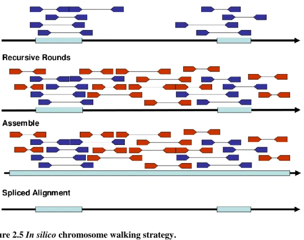
Figure 2.5 In silico chromosome walking strategy. 36

Figure 2.6 Proposed pipeline of SRAssembler. 39

Figure 3.1 Long intron splicing models. 47

Figure 3.2 Confirmation of RSSs. 51

Figure 3.3 Comparison of simulated and real intron sequences. 53 Figure 3.4 The sequence logo around the RSSs in four species. 57

Figure 3.5 Information content plots. 58

Figure 3.6 Length distribution. 60

Figure 3.7 Sequence logo for different subintron length. 64 Figure 3.8 Type I and type III RSSs in the same intron. 65 Figure 4.1 The calculation of the abundances of the primary, intermediate and mature

transcripts. 71

Figure 4.2 The log likelihood of AT1G11020. 78

Figure 4.3 Fragment length distribution of dataset SRR391052. 80 Figure 4.4 Results of transcript proportion estimation of dataset SRR391052. 82 Figure 4.5 Distinguishing isoforms from intermediates. 84 Figure 4.6 Fragment length distribution of dataset SRR360152. 85 Figure 5.1 The integrated mRNA processing model. 90

(6)

LIST OF TABLES

Table 2.1 - The simulation results. 26

Table 2.2 - The results of 11 Arabidopsis genes. 28 Table 2.3 - The results of assembling gene family of peroxisomal biogenesis factor. 29

Table 3.1 - Datasets 49

Table 3.2 - The candidate sites for type I, type II and type III RSSs. 54

Table 3.3 - Confirmed sites. 55

Table 3.4 - Descriptive statistics for length distribution. 59 Table 3.5 - The experimental validated sites found by RSSFinder. 61 Table 4.1 - The length and proportion specified in the simulation of gene AT1G11020. 76 Table 4.2 - The simulation results using uniquely mapped reads with different coverage. 77 Table 4.3 - The estimation of for gene AT1G11020. 78 Table 4.4 - The simulation results using E-M algorithm with different coverage. 79 Table 4.5 - The estimation of for gene AT1G11020. 79

(7)

ABSTRACT

Next generation sequencing (NGS) approaches have become one of the most widely used tools in biotechnology. With high throughput sequencing, people can analyze non-model species at an unprecedented high resolution. NGS provides fast, deep and cheap sequencing solutions, and it has been used to answer various biological questions. In this thesis, I have developed a set of tools and used them to study several interesting research topics. First, de novo whole-genome assembly is still a very challenging technical task. For eukaryotic genomes, de novo assembly typically requires computational resources with very large memory and fast processors. Instead of trying to assemble the whole genome as done in previous approaches, I focus on efficiently reconstructing the genomic regions related to the homologous protein or cDNA sequences. I have developed SRAssembler, a local assembly program using the iterative chromosome walking strategy to assemble the loci of interest directly. Second, I used high-throughput RNA sequencing (refered to as RNA-Seq) data to analyze different intron splicing models and their relative frequency of occurrence. The first mechanism I explored is the recursive splicing patterns in large introns. I have implemented a pipeline called RSSFinder, which can search for recursive sites confirmed by RNA-Seq data. My study suggests the prevalence of recursive splicing in different species. These predicted recursive sites can also be used to investigate certain diseases associated with abnormal splicing of transcripts. In addition, I have demonstrated the use of RNA-Seq data to decipher the detailed mechanisms involved in splicing and their relationship with transcription. Here I proposed mathematical models to estimate the distribution of mRNA splicing intermediates. I

(8)

evaluated my models with simulated data and an Arabidopsis thaliana dataset. My results indicate that co-transcriptional splicing is widespread in Arabidopsis thaliana.

(9)

CHAPTER 1 GENERAL INTRODUCTION

In 1990, an ambitious project called Human Genome Project [1] had started a new era of genome biology. The original plan for this project was conservative and laborious. In order to get the correct sequence order, each piece of DNA sequence must be mapped to markers or signposts before the targets could be sequenced. In 1998, a new approach named shotgun sequencing was proposed by Craig Venter [2], and he announced that the human genome draft would be finished by the end of 2000. This method uses computer programs to piece the fragments together by finding the overlapping sequences. Venter finished the first draft on June 26, 2000, demonstrating the power of automatic computer assembly programs. Based on the idea of shotgun sequencing, a new parallel sequencing technology has been introduced for genome analysis. This so-called next generation sequencing (NGS)

technologies has revolutionized the genomic research. NGS provides fast, deep and cheap sequencing solutions, and it has been widely used to answer various kinds of biological questions. NGS also promotes the studies of non-model species at very low costs. The genome of these species can be assembled using NGS de novo assembly programs. NGS is also used to sequence RNA molecules, also known as RNA-Seq. In addition to the gene expression studies, RNA-Seq can be used to examine the microcosmic mechanisms in

transcriptome such as small nuclear RNAs or intron splicing thanks to the depth of RNA-Seq reads.

In this thesis, I answer some computational and biological questions using NGS technologies. The first question is that instead of assembly whole genome, how can we efficiently assemble the interested genes only? The fundamental problem of whole genome

(10)

de novo assembly is that it requires very expensive computer resources with very large memory (hundreds of GB). In many cases, biologists are interested in a few genes only. For this purpose, I propose a local assembly algorithm which can efficiently assemble the loci of interest with lower computational resources. The second question is how are the long introns spliced? I use the RNA-Seq reads to search for the evidence of recursive splicing, which is a stepwise intron removal mechanism proposed by [3]. The third question is whether splicing is co-transcriptional? How are the relative abundances distributed among the splicing intermediates? Since RNA-Seq is so deep that many reads are mapped to introns or

exon/intron junctions, I can take advantage of this information to estimate the distribution of mRNA intermediates using mathematical models.

The rest part of this chapter will focus on the background information about NGS and splicing mechanisms. I will also describe the splice site prediction tools as well. Chapter 2 is focused on the local assembly algorithm using genomic reads. Chapter 3 and 4 are focused on intron splicing using RNA-Seq datasets.

Next generation sequencing

Next generation sequencing (NGS) has become one of the most promising bioinformatics technologies over the past five years. In this section, I will describe the background information about NGS platforms, basic strategies dealing with NGS reads (mapping and assembly) and its applications.

(11)

NGS platforms

The first NGS system was introduced by Roche 454 [4] in 2005. Illumina GA [5] and ABI SOLiD (Sequencing by Oligo Ligation Detection) [6] are then released in the following years. These three platforms are the most typical and popular NGS platforms. The advantage of 454 system is the sequencing speed and the longer read length. The read length of first generation 454 machine is around 150bp. The newer 454 GS FLX system can generate one million reads with read length 700bp in one day. Another well-known NGS platform is SOLiD, which uses unique two-base color space coding. Each base is checked twice therefore producing more accurate base-calling. SOLiDv4 can sequence up to 1.4 billion paired-end reads (the fragments are sequenced from both ends) in two weeks. Illumina offers highest throughput. For example, Illumina HiSeq2000 can produce 600Gb per run with read length 100bp in 8 days. The cost of HiSeq 2000 is only $0.02 per million bases [7], which is cheapest compared with 454 and SOLiD. A newer MiSeq sequencer was released in 2011. It could produce 150bp paired-end reads with 1.5Gb per run in 10 hours including the library preparation time. MiSeq and Ion Personal Genome Machine (PGM) are targeted to clinical applications and small labs.

One of the major problems of NGS is the sequencing error. Like Sanger sequencing, NGS sequencers also provide the quality score indicating the probabilities of base error using phred algorithm [8]. This algorithm assigns a quality value for each base. In Sanger phred, the quality scores is calculated by , where p is the probability of the base call is incorrect. Each sequencing platform has different error profiles. In Sanger phred, the quality scores are from 0 to 93, and they can be represented by ASCII code 33-126 in plain text sequence files. The quality scores range in Illumina 1.0 is from -5 to 40 (ASCII code

(12)

59-104). But the quality values range has returned to Sanger format after Illumina 1.8. The SOLiD system uses Sanger quality scores based on the color call of two bases. The range is from 0 to 45.

Since Illumina sequencers can generate highest throughput of NGS reads, they have become the most dominant platform in this field. One of the main problems of Illumina reads is the read length. In the library preparation step, the DNA or RNA molecules are chopped into smaller fragments. Each fragment can be sequenced from one end up to 150bp only. The first form of Illumina reads is single-end. That is, only one end of the fragment can be

sequenced. The major problem of single end reads is the ambiguity when reads are mapped to multiple loci. A simple improvement to the single-end library preparation is to sequence both ends of fragments (scanning both the forward and reverse template strand). The paired-end sequencing incorporates the fragment length information which can significantly improve the mapping and assembly accuracy. The typical fragment length of paired-end sequencing is 200-500bp. In terms of genomic assembly, this fragment length is still too short when scaffolding contigs. A newer library preparation method can produce paired reads (referred to as mate pairs) separated by longer distance (2kb ~ 8kb). In this method, longer fragments are circularized and both ends are sequenced. Mate pairs reads are very useful for

the de novo genome.

Mapping strategies

If the reference genome is available, the straightforward way to deal with NGS reads is to map the reads back to the reference sequences. Sequence alignment is an old

(13)

dynamic programming such as Smith-Waterman algorithm [9]. The drawback of dynamic programming is the speed. Some faster alignment algorithms such as BLAST indexes k-mers and they can efficiently pinpoint the location. These k-mer seed sequences are then extended using traditional alignment methods [10]. But these methods are not designed to handle millions of very short reads. Therefore, the new NGS aligners are rapidly introduced and have become one of the prosperous fields in bioinformatics. To promote the aligning efficiency, these aligners only allow small number of mismatches, insertions and deletions. For example, for the read length 36bp, a read can be split into 4 sub-reads with 9bp. If only two mismatches are allowed, two out of four sub-reads must be exactly matched. Therefore, the potential matched reads can be efficiently identified. ELAND [11], ZOOM [12], SeqMap [13] and SOAP [14] are all the aligners based on such principle by building a hash table of substring of length k from either for the reads or the reference sequences.

The main drawback of these programs is the requirement of memory. Bowtie [15], one of the most successful NGS aligner, uses Burrows-Wheeler transform (BWT) based on full-text minute-space (FM) index. The size of FM index is small enough to load it to the memory of a typical personal computer. For example, the memory footprint for human genome needs only about 1.3 GB RAM. The newer version of SOAP [16] and BWA [17] are also used BWT as the indexing strategy.

Assembly strategies

If the reference genome is not available, the NGS reads must be assembled directly. The biggest challenge of de novo assembly is the short read length. If the target regions contain repeat sequences, then these regions become indistinguishable. In fact, the assembly

(14)

programs of whole genome shotgun (WGS) sequencing were developed before the advent of NGS. But these conventional assemblers such as PCAP [18], Arachne [19] or Celera

Assembler [20] are unable to deal with the massive number of microreads. These assemblers employ the Overlap/Layout/Consensus (OLC) three phases approach to find the consensus sequences. The overlap phase involves the pair-wise comparison of all reads using

pre-computed k-mer seeds. Then the approximate read layout is constructed by the overlap graph. Finally, the multiple sequence alignment is used to determine the precise read layout, thereby obtaining the final consensus sequences. This method can still be used to assemble longer and low throughput NGS reads. For example Newbler [21] is a very successful assembler based on this approach, which is widely used to assemble 454 reads.

To assemble large number reads produced by Illumina or SOLiD sequencers, many assemblers have been developed based on the de Bruijn graphs [22] such as Velvet [23], ABySS [24], ALLPATH [25], and SOAPdenovo [26]. The principle of de Bruijn graph is to represent a sequence as a set of k-mer components. Figure 1.1 demonstrates examples of the de Bruijn graph. In these examples, each node represents a 10-mer sequence. If the 10-mer sequence can be found in two sequences, the node will be shared by them. When k is very large, the more memory is required to process and store the graph.

For de novo genome assembly, fragment length information is crucial to obtain

quality results. The better strategy is to assemble multiple libraries including mate pair reads. Such tasks require extremely high computer resources. For example ALLPATH and Velvet need hundreds of GB RAM to assemble eukaryotic genomes using multiple libraries.

(15)

Assemblies are usually evaluated by the size of assembled contigs including average contig length, maximum contig length, total contig length and N50 length. The N50 is the shortest contig length in the set representing at least 50% combined length of the assembly.

Choosing the best parameters is the key to the success of the assemblies. For example, different k-mer may produce totally different assemblies. One may need to try different k-mer and select the assembly producing the best N50 value.

Figure 1.1 The de Bruijn graph.

(A) A NGS read can be represented as a set of k-mer substrings. In this example, k=10. Each 10-mer sequence is denoted as a node in the de Bruijn graph. (B) If a 10-mer sequence can be found in two sequences, the node will be shared by them.

In addition to the genome assembly, RNA-Seq reads can be assembled without a reference genome. The transcriptome de novo assembly is even more challenging than the genome assembly because the coverage of RNA-Seq is not evenly distributed. When the coverage is too low, higher k-mer may yield poor results. Therefore, a single k-mer may not

(16)

generate an optimal assembly. To overcome this problem, several transcriptome assembly programs such Trans-ABySS [27] and Velvet/Oases [28] can produce a set of assemblies using different k, and then merge them together to get the best assembly. Like whole-genome assembling, running the transcriptome assembling also requires very large memory. For example, Trinity [29] needs around 1GB RAM to process one million reads.

NGS applications

Applications of the NGS technologies include the genetic variation detection [30-32], DNA methylation [33-35] and Chip-Seq [36-38]. Other applications have been used to sequence mRNA and small nuclear RNAs and allow global measurement of transcript abundances. Before the development of RNA-Seq, transcriptome analysis [39] relied on the hybridization based[40, 41] or tag sequence-based approaches [42]. RNA-Seq has several advantages over these approaches. For example, RNA-Seq can be used to detect novel genes or transcripts [43-47]. RNA-Seq also has lower background signal and no upper limit for quantification, therefore getting a larger dynamic range of expression levels than microarray analyses [48].

Mechanisms of pre-mRNA splicing

Split genes

Introns were first found by Philip Sharp in 1977 [49]. In their experiments with adenoviruses, they hybridized RNA to the DNA template and inspected them by electron microscopy. Their found that the RNA-DNA hybrids are interrupted by DNA loops, suggesting the information encoded in genes is not continuous. The coding and non-coding

(17)

part of genes is referred to as exons and introns respectively. When mRNA is synthesized in eukaryotes, the mRNA precursors still contain introns transcribed from DNA template. The introns are then removed and adjacent exons are ligated. The origin of introns is still not completely known. At first, processing these useless components appears very wasteful in terms of energy consumption, but today we know the existence of introns largely facilitates the diversity of gene products. The intron removal may involve different pathways, thereby producing functional distinct mRNA isoforms from a single gene. This mechanism is known as alternative splicing. Exons often encode independent functional domains. Therefore, alternative splicing provides a complex design to assemble different functional modules. This is an economic way to achieve the proteome diversity. Furthermore, introns can also play the cis-regulatory roles in splicing. For example, the intronic enhancers and silencers can

promote or inhibit the splice site recognition. The length of introns affects the efficiency of transcription as well, and then the gene expression can be regulated.

Pre-mRNA splicing

To accurately splice the primary mRNA molecules, the exon and intron boundary must be correctly recognized first. The observation of intron sequences reveals that almost all introns begin with dinucleotide GU (5’ donor site) and end with dinucleotide AG (3’ acceptor site). This GU/AG motif is also known as core splicing signals. The branch point, an adenine nucleotide, is a key position to form the splicing lariat (described later), is located at 20-100bp upstream of the acceptor sites. The mammalian consensus intron sequence can be denoted as:

(18)

where exon/intron boundary is denoted by slashes. Y is pyrimidine, R is purine, A is the branch point, and N is any base. Note Yn is a stretch of pyrimidine known as polypyrimidine tract, which is known to promote the recognition of acceptor sites.

Most intron removal is catalyzed by spliceosome, a complex containing small nuclear ribonucleoproteins (snRNPs) and other protein factors. snRNPs contain the RNA molecules which can pair with mRNA sequences. There are two types of spliceosomal splicing

pathways: the canonical and non-canonical. The canonical pathway accounts for 99% of splicing. The aforementioned GU/AG is the motif sequence of canonical splicing. The canonical spliceosomal splicing cycle begins with the recognition of 5’ splice site by U1 snRNP. The branch point is then bound by the splicing factor SF1. The U2 Auxiliary Factor (U2AF) also interacts with 3’ splice site and the polypyrimidine tract. Next, the U2 snRNP binds to the branch-point and join to form the “A complex”. Another U4/U5/U6 tri-snRNP then joins and forms “B1 complex”. Later, U1 is displaced by U6, which pairs with U2. At this point, U1 and U4 are dissociated and the “B2 complex” forms. The 2’OH of the branch-point attacks on the 5’ splice site via transesterification reaction and forms the lariat splicing intermediate and the “C1 complex”. The second transesterification reaction is performed by the attack of free 3’OH of upstream exon on the last nucleotide of the intron, forming the “C2 complex”. The C2 complex joins the exons and releases the lariat, which is then degraded.

In the non-canonical pathway, the motif of exon/intron boundary is AU/AC. Since the consensus intron sequence is different, the splice site recognition is done by another group of spliceosomes. The roles of U1, U2, U4 and U6 is replaced by U11, U12, U4atac and U6atac snRNPs respectively.

(19)

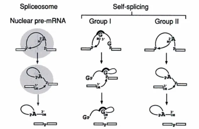
In addition to the spliceosomal introns, some introns can be spliced without the help of a spliceosome. These self-splicing RNAs can be classified into two groups. The group I introns was first discovered in 26S rRNA gene of Tetrahymena by Thomas Cech [50]. Group I self-splicing occurs via the process that a guanine nucleotide in the intron attacks adenine nucleotide at the 5’ end. Then the OH group at the upstream exon attacks the downstream exon, releasing the linear intron. The group II self-splicing acts very similar to the

spliceosomal splicing, including the transesterification by the branch-point. The introns then form a secondary structure akin to the spliceosomal lariats (Figure 1.2).

Since the motif of donor and acceptor splice sites has very low information content. The true splice sites must compete with many false ones. This problem may become even worse when the intron size is very large. In fact, the splice site recognition is promoted by a group of extrinsic factors such as SR proteins or hnRNP (heterogeneous nuclear

ribonucleoparticles) proteins. SR proteins contain one or more serine and arginine-rich domains and can interact with RNA via RNA Recognition Motifs (RRMs). The cis-acting splicing regulatory elements such as exonic splicing enhancers (ESEs) or exonic splicing silencers (ESSs) can interact with SR proteins and hnRNP proteins to promote and inhibit the splicing.

As mentioned earlier, the splice sites can be recognized by the ends of introns. This is also known as “intron definition”. Today we know the mechanism of intron definition is prevalent in shorter introns. The splice sites can be bridged across the introns by the

spliceosomal components and the extrinsic proteins. In longer introns, however, some splice sites can be recognized by both ends of exons (referred as to “exon definition”)[51]. In this case, mutation of the splice sites will cause intron retention instead of exon skipping.

(20)

Figure 1.2 Spliceosomal splicing and self-splicing.

Both spliceosomal and group II self-splicing involve the attack of OH group at branch-point. The group I splicing shows a distinct splicing mechanism contains the attack of a guanine nucleotide[52].

Alternative splicing

Some genes can produce more than one isoforms because of different splicing patterns. This mechanism is also known as alternative splicing. Alternative splicing is

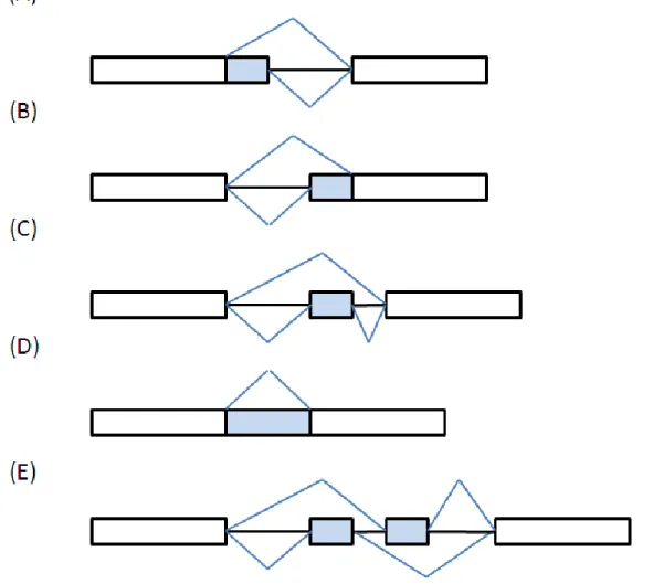
prevalent in eukaryotic genes. For example, a human transcriptome study by high throughput sequencing indicates that more than 95% human genes undergo alternative splicing [53]. Alternative splicing can be classified into five categories (see Figure 1.3):

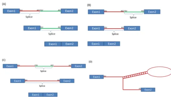
1. Alternative donor site: An alternative upstream exon boundary used. 2. Alternative acceptor site: An alternative downstream exon boundary used.

(21)

3. Exon skipping: An exon may be retained or removed. 4. Intron retention: An intron may be retained or removed. 5. Mutually exclusive exons: Only one of two exons is retained.

Figure 1.3 Alternative splicing patterns.

(A) Alternative donor site. (B) Alternative acceptor site. (C) Exon skipping. (D) Intron retention. (E) Mutually exclusive exons.

Different alternative splicing patterns can be regulated by trans-acting proteins or cis-acting elements. For example, some intronic sequences may encode microRNAs, which may inhibit the isoform expression via RNA interference (RNAi) pathways [54]. In some cases,

(22)

alternative splicing may disrupt the open read frame by introducing frameshifts or early immature stop-codons. The mRNAs with abnormal stop-codons may be degraded through the nonsense mediated decay (NMD) pathway [55], but other abnormal splicing might contribute to diseases or genetic disorder [56, 57]. In short, alternative splicing plays a crucial role in biodiversity, diseases, gene expression regulation.

Splice site prediction and RNA-Seq alignment

Splice site prediction

After part of splicing mechanism has been deciphered, several tools have been developed to find the splice junctions given a piece of DNA sequence. These tools typically use the context information around the known splice sites to predict new splice sites from the genomic sequences alone, without mRNA evidence. For example, SplicePredictor [58] predicts splice sites by measuring the intrinsic splice site quality [59], local optimality of the site, and the contribution of the sites to the splicing patterns in the context of the flanking sequence segments. GeneSplicer [60] uses similar Markov modeling to predict Arabidopsis thaliana and human splice sites. Several machine learning based splice site detectors are also reported to perform at a very good level [61-65].

Spliced alignment for RNA-Seq data

Traditionally, transcript discovery and gene annotation have relied on the alignment of full-length cDNAs or ESTs as well as homologous protein sequences to the genomic sequences being annotated. Such spliced alignment tools include NAP [66], Genewise [67], Blat [68], GeneSeqer [69] and GMAP [70]. This strategy allows long alignment gaps in the

(23)

mapped transcripts or proteins that correspond to introns in the reference genome. However, traditional spliced alignment methods are not directly applicable to RNA-Seq because they need longer sequences that cover the exon-exon boundary for the reliable gene structure prediction. For example, suppose a read maps on the exon-exon junction in such a way that only few bases are within one of the exons. In this case, traditional dynamic programming methods trying to make the spliced alignment across a potential long intron are ineffective. Aforementioned NGS aligners can rapidly map reads to reference genomes. But these tools allow only small number of mismatches, insertions and deletions. Some NGS spliced alignment tools such as Tophat [43, 45] or G.Mo.R-Se [43] assemble all mapped reads into potential exon islands. The candidate exon junctions could then be obtained by searching within a specific window around the island boundary, say 100 nucleotides. The possible donor and acceptor sites could be determined by the terminal dinucleotide pairs, such as canonical GT-AG splice sites. All possible splice sites are tested by the reads that were not mapped initially. However, these methods may incur too many false-positives. On the other hand, algorithms like ERANGE [71] or RNA-mate [72] use a known annotated junction libraries. Therefore, this method is generally limited to the cases that we only intend to know the expression levels instead of discovering novel junctions. Other spliced alignment tools use the splice site prediction models to improve the accuracy of the junction discovery. For example, QPALMA [44] applies machine learning techniques to train a support vector machine from known splice junctions. GSNAP [73] can evaluate the surrounding genomic sequence using probabilistic models of splice sites.

(24)

Research goals

The work in this thesis focuses on using NGS data to answer several computational and biological questions. Below I introduce the goals of my three main topics. In chapter 2, 3 and 4, I will describe my methods and results for them in detail.

Local assembly of homologous regions by genomic DNA reads

For eukaryotic genomes, de novo assembly typically requires the computer resources with very large memory and fast processors. Even with such extensive computational

resources, an assembly may still take several days to finish. However, sometimes biologists are only interested in small set of genes with known homologous protein sequences. My goal is to design an algorithm to quickly and accurately assemble the loci of interests. I have developed a program called SRAssembler (Selective and Recursive local Assembler), which is shown to be able to do the local assembling efficiently using iterative chromosome

walking strategy.

Genome-wide survey of stepwise intron removal by RNA-Seq data

Stepwise intron removal has been shown an important mechanism in Drosophila. However, only very small number of recursive sites can be validated. My goal is to use RNA-Seq data to search for the stepwise intron removal evidence including two types of recursive splicing and intrasplicing. I have developed a pipeline called RSSFinder (Recursive Splice Sites Finder) to investigate the recursive splicing mechanisms in four species

(25)

Splicing intermediates analysis using RNA-Seq data

The mechanisms of transcription and splicing are two interactive processes. The splicing pathways could be very complex with many possible mRNA intermediates. Since RNA-Seq data is so deep that many reads are mapped on intronic regions, I can use the RNA-Seq reads to estimate the distribution of mRNA intermediates. I used simulation data to evaluate the performance of my algorithms. I also use this model to examine the Arabidopsis genes with 3 and 4 exons. My study may serve as the foundation to further understand the splicing dynamics and the relationship between splicing and transcription.

(26)

CHAPTER 2 SRASSEMBLER: LOCAL ASSEMBLY OF

HOMOLOGOUS REGIONS BY GENOMIC DNA READS AND

HOMOLOGOUS GENES

A paper to be submitted to Genome Biology Hsien-chao Chou1, Volker P. Brendel 2,3*

Abstract

We have developed a tool, SRAssembler, which locally and recursively assembles the genomic reads associated with the homologous query genes. We demonstrate SRAssembler can successfully and efficiently reconstruct loci of interest from several datasets. It has several advantages over the whole genome de novo assembly such as the running time and required computing resources. The contigs assembled by SRAssembler can also be used to evaluate the quality of whole genome assemblies. The source code is available at

http://grinch6.gdcb.iastate.edu/~hchou/SRAssembler/.

1

Department of Genetics, Development & Cell Biology, Iowa State University, Ames, Iowa 50011, USA

2

Department of Biology, Indiana University, Bloomington, Indiana 47405 3

School of Informatics and Computing, Indiana University, Bloomington, Indiana 47405

(27)

Rationale

Next generation sequencing (NGS) approaches have become one of the most widely used biotechnology tools [74]. Applications of NGS include the generation of detailed maps of genetic variation [31, 32, 75], DNA methylation [33, 34], and transcription factor binding sites (Chip-Seq) [36, 37]. NGS technologies also provide opportunities to de novo sequence genomes of non-model species at very low costs. Because NGS relies on extensive sequence coverage with small reads, accurate assembly of the reads to large contigs, scaffolds, and pseudochromosomes is an intrinsic part of the approach. A large number of NGS assembly tools have been developed for this purpose. Based on de Bruijn graphs [76], such programs have been shown to effectively handle millions of short reads, including, for example, ABySS [24], ALLPATH [25], and SOAPdenovo [26].

Current challenges in assembly focus on increasing average contig size, usually measured as N50 size (N50 is the median length of contigs. People usually use it to evaluate the quality of the assembly) [77], and reducing error rates. Some strategies have been introduced to deal with these problems, such as gene-boosted assembly [78] and homology-guided assembly [79]. The assemblies based on highly related genomes have been shown to produce better results by incorporating homologous sequence information. Another challenge with de novo assemblers is that assembling the massive amounts of data is still a very difficult technical task. For eukaryotic genomes, de novo assembly typically requires computational resources with very large memory and fast processors. Even with such extensive computational resources, an assembly may take several days to complete even for a single run, and, depending on the complexity of the input data, it may not finish at all. Furthermore, if the resulting assembly is not satisfactory, parameter adjustments and

(28)

subsequent runs and comparative evaluation of different draft assemblies are typically required. These challenges must inevitably be overcome ultimately to get a reliable whole-genome assembly. For example, one of the most important parameter is the k-mer value, which is the overlap length in the de Bruijn graphs. In most cases, we do not know how to assign the best k value. The only solution seems that we need to try different k value and pick the one with the best N50 size.

Whole-genome assembly is not necessarily the immediate nor the only goal of genome-wide NGS approaches. Because of the cost-effectiveness of NGS technologies, a research group may well choose genome-wide NGS for a species even if they are interested in only a subset of the species’ genes, for example, homologs of genes already identified in other species as involved in a specific biochemical pathways or cellular structures. In those cases, it becomes desirable to restrict the assembly to those genic regions only; that is, instead of assembling the entire genome, we want to assemble the reads which correspond to annotated homologous genes of interest only. Adopting this strategy enables us to focus the assembly on specific regions, drastically reducing the required resources and running time. In pursuit of this goal we have developed the program SRAssembler (Selective and Recursive local Assembler). SRAssembler uses protein or cDNA sequences from a related species as query input to find and assemble NGS reads from a novel sequencing project for a species of interest. Potentially homologous reads serve as queries for the next recursive round of assembling local contigs, representing essentially an “in-silico” chromosome walking

strategy as originally developed for mining the now outdated NCBI trace archive with the Tracembler program [80]. User can specify the success criteria that determine the break

(29)

condition for the recursion. At the last stage, the original queries are spliced aligned to the draft contigs and the potential gene structures are identified.

SRAssembler is implemented as a C++ program that relies on a number of external programs for string matching, assembly, and spliced alignment. Default pre-requisites are Vmatch [81, 82], SOAPdenovo [83], Bowtie [15], and GenomeThreader [84]. It supports Message Passing Interface (MPI) [85] parallel computing. The reads data can be split into several parts so that the local alignment can be executed at the same time, therefore speeding up the running time. In each round of the recursion, different values of k-mer, the overlap length parameter in the de Buijn graph analyses, are tested simultaneously. Since the k-mer parameter significantly affects the quality of assembly, different k-mer should be tested in order to find the best one. The criterion to pick the best assembly is by evaluating the length of contigs produced. The assembly that produces the longest contig is considered the best assembly.

Here we demonstrate SRAssembler can successfully assemble the Arabidopsis thaliana loci by Oryza sativa (rice) protein sequences. In this case, it is seen that SRAssembler can distinguish and recover all the related paralogous genes even their similarity is very high. We also show the SRAssembler could serve as an ideal tool to evaluate the quality of whole-genome assemble by testing the core eukaryotic genes.

(30)

Results and discussion

Assembly of homologous loci from simulated data

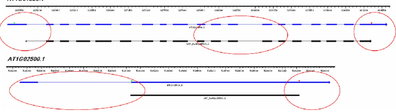
As a first test of the applicability of the SRAssembler strategy to construct local assemblies of NGS reads that would encode putative homologs of query protein probes, the program was tested on simulated read data from Arabidopsis chromosome 1 in pursuit of assembly of (known) homologs of two representative rice proteins. The two rice genes were accessions OS01G18860.2 (S-adenosylmethionine synthetase, putative, expressed) and OS06G04560.1 (armadillo/beta-catenin repeat family protein, putative, expressed), with unique Arabidopsis homologs AT1G02500.1 (SAM1) and AT1G01950.1 (ARK2), respectively. Figure 2.1 depicts the gene structure of the Arabidopsis genes and a spliced alignment of the rice proteins onto the Arabidopsis genome sequence produced by GenomeThreader [84]. AT1G02500.1 is a relatively short gene structure consisting of only two exons, with the upstream exon entirely 5’-UTR (and therefore not covered by the rice protein spliced alignment). AT1G01950.1 is a 19-exon gene structure spanning 5,241bp and represents a relatively long gene model in Arabidopsis. The detailed exon alignment scores are shown in Table S1. There are 4 exons whose alignment scores are lower than 0.5. (The score range is from 0 to 1). Moreover, the average exon length of this gene is 132bp, which is relatively short compared to the average exon length 185bp in rice and 155bp in Arabidopsis [86]. The short average exon length as well as a poorly conserved internal region (circled in Figure 2.1) should make local assembly of this locus based on the initial protein query challenging.

(31)

As a measure of success of SRAssembler, the longest assembled contig was matched against the known Arabidopsis locus. Results are shown in Table 2.1. Depending on the simulated read coverage, SRAssembler assembled partial or complete loci, including the UTR and divergent internal regions. At 25X chromosome coverage, both loci were assembled completely and correctly.

Figure 2.2 demonstrates the recursive sampling strategy employed in SRAssembler by example of the AT1G01950.1 assembly. For each recursion round, all reads identified thus far as potentially part of a homologous locus were mapped to the final contig (using Bowtie [15]) and visualized with the Integrative Genomics Viewer (IGV) [87]. It is seen that in the initial round, all reads are locally aligned to the exons. Because the simulation was based on paired-end reads, both ends of the reads will be included as long as either one of them was mapped to an exon part, which makes the in silico chromosome walking in part more akin to “chromosome jumping”. Note that, expectedly, no reads are aligned to the long central intron in the middle in the first round. In the round 3, we can see more and more reads filling out adjacent regions. In the round 5, whole region is covered by reads. These reads are assembled into a complete contig with 100% identity compared to the TAIR10 genomic sequence [88].

(32)

Figure 2.1 The spliced alignment of OS01G18860.2 and OS1G04560.1.

We used GenomeThreader to align these two rice genes, accessions OS01G18860.2 and OS1G04560.1 (black) to Arabidopsis genome. We also show the gene structure of their homologous genes AT1G02500.1 and AT1G01950.1 (blue). The unconserved regions are highlighted by red circles, including the 3’ UTR, 5’ UTR and three exons in AT1G01950.1.

(33)

Figure 2.2 Chromosome walking of gene AT1G01950.1.

We mapped the reads of each round back to the final contig. The blue bars are the exons predicted by GenomeThreader. Mapped reads are shown as either red or light blue arrows, representing forward and reverse orientation respectively. In the initial round, all exons are locally aligned by reads. Because we used paired-end reads, some introns are also mapped if either end is mapped to the exon part. As the iteration goes, reads are mapped toward the long intron part in the middle and the both ends of the target locus.

(34)

Table 2.1 - The simulation results.

The simulation results of two Arabidopsis genes, accessions AT1G01950.1 and

AT1G02500.1. We simulated reads data with coverage from 10X to 25X. We used BLASTN to align our contigs to the gene loci. The target loci length is 5,240 and 2,186 respectively. The aligned length refers to the length in the target loci successfully covered by

SRAssembler contigs. The identity is the percentage of identical nucleotides in the aligned regions. The results show that both genes are correctly assembled when the read coverage is 25X. AT1G01950.1 (Locus length: 5,241) AT1G02500.1 (Locus length: 2,187) Reads Pairs Reads Coverage Aligned Length Aligned Percentage Identity Aligned Length Aligned Percentage Identity 2,173,405 10X 1,681 32% 99% 693 31% 99% 3,260,107 15X 1,879 36% 100% 1252 57% 100% 4,346,810 20X 5,241 100% 100% 1023 47% 99% 5,433,512 25X 5,241 100% 100% 2187 100% 100%

Assembly of homologous loci from real data

In real experiments, NGS reads are typically not uniformly distributed over the genome sequence. To test SRAssembler performance over a wider range of potential applications with varying local read coverage as well as varying query to assembled gene product similarity, we selected loci from the Arabidopsis chromosome 1 segment from 200,000 to 1,000,000. The PlantGDB AtGDB rice homologs track [89] indicated 11 loci in that range that are at least 20kb apart and have rice homologs. Results of SRAssembler with the 11 rice proteins as query are shown in Table 2.2. Typically SRAssembler assembles many contigs including those we are not interested in. The GenomeThreader [84] can

normally reduce the number of contigs to less than 10. In most cases, they are from partial or complete duplication events. In this test, we used BLASTN to align these contigs to

(35)

interests. For most of the loci, SRAssembler successfully assembled contigs with high identity and coverage scores. The evolutionary distance information is obtained by

GreenPhyl website [90]. The most distant genes are AT1G02830.1 (Ribosomal L22e protein family) and OS3G22340.1 (60S ribosomal protein L22-2, putative, expressed), whose evolutionary distance is 0.36. But this locus can be assembled without any problems. The actual evolutionary distance was computed using PROTDIST from package PHYLIP [91]. For some genes we did get the very good aligned percentage for whole loci, but we got very good results if we consider the coding region only (See column 8 in Table 2.2). For example, the aligned percentage of whole locus for gene AT1G02500.1 is only 52% for the entire locus including UTR regions, but it was 96% for the coding region.

(36)

Table 2.2 - The results of 11 Arabidopsis genes.

This table shows the results of the local assembly of 11 genes. The locus start and end are the coordinates of the loci of the Arabidopsis genes. We used BLATN to align SRAssembler contigs to the genomic sequences. The contig start and end indicate the regions mapped by SRAssembler contigs. The aligned percentage refers to the proportion of target regions can be aligned by SRAssembler contigs. We can see we can get better aligned percentage if we consider the coding regions only. The evolutionary distance also provides the information how these two homologous genes are related.

Arabidopsis genes Oryza Sativa genes Locus Start Locus End Contig Start Contig End Aligned Percentage - Whole Locus Aligned Percentage - Coding Region Evolutionary Distance AT1G01560.1 OS08G06060.1 202,136 204,335 202,531 204,754 82% 86% 0.23 AT1G01750.1 OS02G44470.1 275,366 276,310 274,587 277,586 100% 100% 0.21 AT1G01820.1 OS06G03660.1 296,001 298,120 295,028 298,873 100% 100% 0.23 AT1G01950.1 OS06G04560.1 325,379 330,619 325,292 331,411 100% 100% 0.14 AT1G02130.1 OS01G08450.1 400,035 401,882 400,358 402,227 82% 100% 0.07 AT1G02500.1 OS01G18860.2 518,251 520,437 519,028 520,172 52% 96% 0.08 AT1G02830.1 OS03G22340.1 625,145 625,608 625,022 627,834 100% 100% 0.36 AT1G03190.1 OS05G05260.1 775,527 780,027 774,628 779,739 94% 97% 0.18 AT1G03330.1 OS8G05850.1 817,983 819,563 817,634 820,053 100% 100% 0.2 AT1G03475.1 OS4G52130.1 869,051 871,211 868,725 871,723 100% 100% 0.23 AT1G03630.1 OS10G35370.1 907,642 909,376 906,858 909,850 100% 100% 0.24 Paralogous genes

Since gene duplication is a very common event in plant species, it is important to identify and assemble these paralogous loci. Here we also tested if SRAssembler can distinguish and assemble the paralogous genes. For Arabidopsis gene AT1G01820.1 (PEX11C), which is a member of peroxisomal biogenesis factor 11 family, we have two other paralogs located in chromosome 2 and 3 respectively. In Table S2, we summarize this gene family. This gene family information is obtained from Inparanoid web site [92]. Now

(37)

we used their rice homologous gene, OS6G03660.1 (Peroxisomal membrane protein PEX11-1, putative, expressed), to test if we can find all these three loci. The results are shown as Table 2.3. We can see SRAssembler successfully assembled all paralogous genes.

Table 2.3 - The results of assembling gene family of peroxisomal biogenesis factor. We demonstrate SRAssemble can perfectly identify all paralogs of gene family peroxisomal biogenesis factor 11 in Arabidopsis. The three paralogs are located in chromosome 1, 2 and 3. The locus start and end are the coordinates of the loci of the Arabidopsis genes. We used BLASTN to align SRAssembler contigs to the genomic sequences. The contig start and end indicate the regions mapped by SRAssembler contigs. The identity is the percentage of identical nucleotides in the aligned regions. We can see that the target regions are completely covered by SRAssembler contigs. The evolutionary distance is the distance between

Arabidopsis and the query rice genes.

AT genes OS genes Locus

Start Locus End Locus Length Contig

Start Contig End Identity

Aligned Percentage Evolutionary Distance AT1G01820.1 OS6G03660.1 296,001 298,120 2,120 295,901 298,417 100% 100% 0.23 AT2G45740.1 OS6G03660.1 18,839,865 18,841,102 1,238 18,839,137 18,841,713 99% 100% 0.29 AT3G61070.1 OS6G03660.1 22,604,873 22,606,159 1,287 22,604,702 22,606,283 99% 100% 0.29

Core eukaryotic genes

We also used SRAssembler to test core eukaryotic genes. These genes are present and conserved in a wide range of species. There are 458 highly conserved core genes identified by CEGMA (Core Eukaryotic Genes Mapping Approach) study [93]. We examined first 30 such proteins with size larger than 100 amino acids. We used Drosophila melanogaster core genes as query proteins to assemble the homologous regions of Acromyrmex echinatior (leaf cutting ants). Out of these 30 proteins, 25 contigs are identified with good alignment score and coverage in the GenomeThreader report. In the last round of SRAssembler, the k-mer

(38)

value 45 was chosen in terms of the length of contigs. Since we have very high confidence in these contigs, we can use them to evaluate the quality of whole-genome de novo assemblies. We aligned the SRAssembler contigs to four whole-genome assemblies. The first one was assembled by SOAPdenovo with one 500bp library using k-mer value 27. Its N50 value is 1,927bp. We assembled the second assembly with the same dataset as the first one, but used

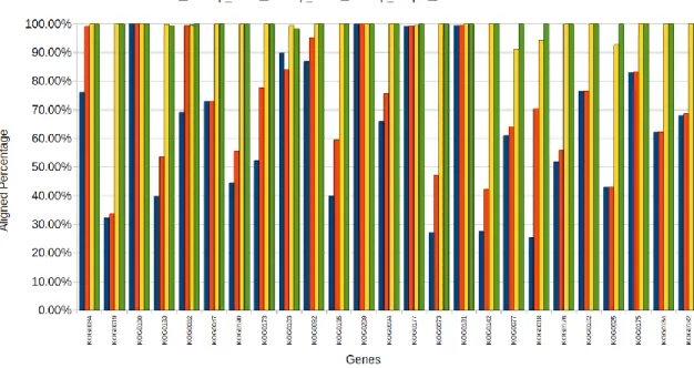
k-mer value 45, which is determined by the last round of SRAssembler. This assembly has N50 value 2,346. For the third assembly, we used an additional 2kb mate-pair library, whose N50 is 4,326bp. The last one is the assembly submitted to NCBI whole genome shotgun sequencing project by Beijing Genomics Institute (accession no. AEVX00000000) [94], which contains 4 libraries with various insert size. Its N50 is 80,630bp. The Figure 2.3 shows the comparison of these assemblies. The aligned percentage in Figure 2.3 refers to the percentage of SRAssembler contigs aligned to whole-genome assemblies. If a SRAssembler contig can align to multiple contigs in whole-genome assemblies, we simply pick the best one. Our results indicate that quality of the contigs generated by the first assembly is not very good, because they are relatively fragmented when aligned to SRAssembler contigs. Here we got only one contig completely matched. The assembly with two libraries is highly consistent with SRAssembler contigs, showing the better quality of this assembly. We can see that the mate-pair information is very useful to merge short contigs into big ones. The last assembly, with four libraries, performs the best in our comparison. They are almost identical to the SRAssembler contigs. We also noticed that the k-mer value chosen in the first assembly is problematic. Since SRAssembler can test different k value at the same time, we can use the k

(39)

assembly. We can see the significant improvement when we switch k value from 27 to 45. The detailed results are shown as Figure 2.3 and Table S3.

Figure 2.3 Comparison of assemblies.

We assembled 25 contigs from 25 core eukaryotic genes. Then we aligned them to three whole-genome assemblies. We can see the AEVX00000000.1 assembly is highly consistent with SRAssembler contigs, and SOAPdenovo assembly with k-mer 27 is relatively

fragmented. Therefore, we can use SRAssembler contigs to evaluate the quality of whole-genome assemblies.

Running time

Since SRAssembler assembles homologous regions directly, it can finish the assembly in very short time. Here we selected a rice gene accession OS06G03660.1 (Peroxisomal membrane protein PEX11-1, putative, expressed) and aligned it to the 30 million Arabidopsis genomic reads. To understand how parallel computing benefits the running time, we tested the SRAssembler on the TACC Ranger HPC system [95] . The memory capacity is 32GB, but SRAssembler only requires lesser than 2GB in such test run.

(40)

We tested 15 rounds (this is a typical number of rounds) with two datasets. The first one used one library, SRR073127, whose size is 32.4 million reads. The second one has two libraries. In addition to SRR073127, we added another library, SRR071796, which has 30 million reads. The read length for both libraries is 75bp. The resulting contig perfectly covers the target region and the identity is 100%. Here we only focus on the running time. We can see when we have only one core, the execution time is around 147 minutes to finish 15 rounds for two libraries. As we used more CPUs up to 16 cores, we found the execution time dropped to 45 minutes, which means we can correctly assemble a gene out of 60 million reads in 45 minutes. For single library, the running time is only around 35 minutes. The results are shown as Figure 2.4. Note that these results include the pre-processing step, which splits the reads data into smaller ones. This step can be skipped when we rerun the same dataset, which can significantly reduce the running time further.

(41)

Figure 2.4 Running time of SRAssembler.

Since SRAssembler assembles homologous regions directly, it can finish the assembly in very short time. For single core, the execution time is around 147 minutes to finish 15 rounds for two libraries. As we used more CPUs up to 16 cores, we found the execution time

dropped to 45 minutes, which means we can correctly assemble a gene out of 60 million reads in 45 minutes. For single library, the running time is only around 35 minutes.

(42)

Conclusions

SRAssembler provides a new way to assemble the genes of interest directly, which is extremely efficient if people are only interested in a few genes. From the tests we have seen, SRAssembler seems to be able to assemble partial or whole the homologous region correctly. It has several advantages over the whole genome de novo assembly. First, it is much faster. For the rice test cases, with the help of parallel computing, we can find homologous regions within 40 minutes. Second, it requires less resource. For a typical search, 2GB memory is enough for most cases. Third, it is flexible. Since the SRAssembler is implemented as object-oriented framework, it is very easy to add new internal assemblers. Also, different k values can be tested simultaneously. If users have a 16-core machine, 15 different k-mer values can be tested at the same time. Therefore, SRAssembler can quickly select the best k for the whole-genome assembly as shown in the second assembly in the test case of core eukaryotic genes. From the comparison with the whole-genome denovo assembly strategy, we found SRAssembler can generate identical or better results than the global assemblies. Since

SRAssembler can assemble the contigs with very short time, it could serve as a benchmark to quickly evaluate the quality of the global assemblies. For the assemblies of eukaryotic

species without reference genome, we can always use SRAssembler to assemble some of 458 core eukaryotic genes first. Then a good assembly should be able to assemble them correctly no matter how well the N50 value it gets. We believe SRAssembler can serve as a good supplementary tool of whole-genome de novo assembly.

A related approach to iterative targeted and micro NGS assembly was recently introduced in the Mapsembler program [96]. Although Mapsembler also adopts the similar iterative search algorithm as did in Tracembler and SRAssembler, it is not designed to

(43)

assemble homologous loci. Mapsembler is a tool targeting specific biological events such as transposase elements or gene fusion. It cannot handle the case where the similarity between query sequences and NGS reads is not very high (<90%). In our preliminary tests,

Mapsembler cannot assemble any test cases shown in this paper. It does not support protein sequences and paired-end reads as well, which are very useful for the homology search.

Materials and methods

In silico chromosome walking strategy

The basic strategy implemented in SRAssembler is depicted in Figure 2.5. Initially, NGS reads are aligned to a query sequence using the fast string matching program Vmatch [82]. If the query sequence is a protein, the matching is to all possible translations of the reads (Vmatch option -dnavsprot). Default Vmatch parameter settings in SRAssembler are initial matching length 10 for protein sequences and 30 for cDNA sequences. The default mismatches allowed are 1 for protein sequences and 2 for cDNA sequences. The matching length for recursive rounds is 30. These setting can be changed by the user. Retrieved reads from this initial matching are assembled into contigs which become the query sequences for subsequent rounds of in silico chromosome walking. By default, SRAssembler invokes SOAPdenovo for the assembly step. During the assembly step, the assembler is run multiple times with different k-mer values (the default setting is 15, 25, 35, and 45). We assume the best k-mer is determined by the length of longest contig. The contigs produced by the best k -mer will become the query sequences for the next round. The recursion is terminated as soon as one of the following criteria is met: (1) No new reads can be found; (2) A specified maximum number of iterations is reached; or (3) All contigs match or exceed a specified

(44)

maximum length. The spliced alignment program GenomeThreader [84] is used to map the original query onto all assembled contigs.

Figure 2.5 In silico chromosome walking strategy.

The SRAssembler first aligns query sequences to the reads data. The reads initially mapped are shown as blue pairs. Note that both pair will be included as long as either end of the read is mapped. Then these reads serve as seeds to “walk” through the chromosome. The adjacent reads are searched by this “walking” strategy (red pairs). All reads we get will be assembled as contigs, and then the predictive gene structure could be obtained by spliced alignment tools to align the original query sequences to the assembled contigs.

Implementation

SRAssembler is implemented in C++ and compiles with any standard C++ compiler. Input read files can be in either FASTQ or FASTA format. Although SRAssembler accepts single end reads, paired-end reads always provide much better results. SRAssembler also

(45)

supports multiple libraries. Libraries with different insert size can improve the quality of assemblies. For example, some mate-pair reads with very long insert size are very helpful to merge two contigs into a big one. The query sequences can be either protein or cDNA sequences provided in FASTA format. The SRAssembler workflow is shown in Figure 2.6. SRAssembler supports compilation under the Message Passing Interface (MPI) [85]. To realize the MPI protocol, the SRAssembler first splits the input reads file into smaller chunks, which can be aligned on different nodes. One node will serve as the master node, which sends the split read file to slave nodes and finally merges the alignment results as one file. The reads that aligned to the query sequences can either serve as new query sequences in the next round or first be assembled to contigs, depending on the parameter settings. In the latter case, very short contigs will be removed. The remaining contigs become the new query sequences for the next round. In each round, the contig size is checked. If the contig size is larger than the predefined maximum value (default value 10,000), SRAssembler will stop assembling such contigs. Because they are long enough, we do not want to waste our time to keep assembling them again. SRAssembler also remove the reads associated with these contigs, therefore improving the running time. This is done by the following steps:

1. In each round, we test if the contig length is larger than the maximum contig size. We trim the head and tail of the contigs and make their size be equal to the maximum contig size, and then copy these contigs to the candidate long contig file. Note that we do not remove them immediately, because we want to do the double check if these long contigs are correctly assembled. If such contigs are assembled again, we can confirm they are our final contigs.

(46)

2. In the next round, we align the candidate long contigs to the current assembled contig file (done by Vmatch). If matched, we move the contigs to the permanent long contig file.

3. We align current matched reads to the long contigs (done by Bowtie). If matched, those reads are removed from the reads pool.

4. Long contigs are removed from the query file of the next round.

Users can also use option –r to indicate when SRAssembler should remove the reads cannot be mapped to current contigs. For example, assigning –r option 5 will make

SRAssembler do the cleaning every 5 rounds. These reads are considered as “noise” reads, which may affect the accuracy of the assembling and increase the running time.

After the recursion step is done, we use the spliced alignment tools to align the original query sequences to the final contigs. Because the length of reads is very short, some incorrect or irrelevant contigs may be assembled. To evaluate the quality of these contigs, we use the GenomeThreader to map the homologous query sequences to them. If the contigs are the homologous regions of interests, the potential gene structure should be identified by GenomeThreader. In most cases, the contigs with longest predicted open reading frame should be the ones we are looking for.

(47)

Figure 2.6 Proposed pipeline of SRAssembler.

The pipeline takes as input the DNA reads and query sequences. The query sequences could be either cDNA or protein sequences. In the preprocessing step, reads data is split into smaller ones so that we can align them in parallel. Then we use Vmatch to align reads

locally. Alignment reports are merged to one file. Then we use these initial hits as seeds to do the chromosome walking by recursively mapping back to the DNA reads until either no reads found or maximum rounds reached. In each round, we assemble the cumulated hit reads by SOAPdenovo assembler. The assembled contigs are the new query sequences used to find new reads. Finally, we use GenomeThreader to align the original query sequences to the final contig file, thus obtaining the proposed gene structure.

(48)

Simulation

We simulated paired-end NGS sequencing of chromosome 1 of Arabidopsis thaliana using the wgsim program of SAMTools [97]. The number of reads N was calculated as N = (length of chromosome 1 x coverage) / (length of reads x 2). Parameters were set as follows: base error rate 0.02, mutation 0, and the fraction of indels 0.10. Coverage was set to 10X, 15X, 20X, or 25X. Read length was set to 70bp, and insert size to 200bp with standard deviation 50bp.

Datasets

The datasets we used for Arabidopsis thaliana assembly are two libraries from Arabidopsis 1001 Genomes Project. They were downloaded from NCBI SRA database [98, 99]. The total number of spots is 16.2 million for SRR071796; 15 million for SRR073127. Before we can use this dataset, we need to first preprocess it so that we can get higher quality assemblies. We removed low quality reads and trimmed the adapter sequences. Since such preprocessing may cause orphan reads, we shuffled reads into single file so that we can easily deal with orphan reads. We first use the shuffleSequences_fastq.pl of Velvet [23] package to make an interleaved FASTQ file. Then we used ea-utils’ fastq-mcf [100] to filter out the low quality reads and trim the adapter sequences. The resulting file is then split into paired-end reads and single reads, whose number are 30,159,924 and 832,218 respectively. As for the test case of Acromyrmex echinatior, we have three assemblies. The first one was assembled from one Illumina paired-end reads library, whose SRA accession no. is ERR034186 [101]. The insert size of this library is 500bp. The number of paired-end and single reads after preprocessing are 105,032,566 and 875,341. In addition to the library ERR034186, the

(49)

second assembly used another library, SRA accession no. ERR034188 [102], whose average insert size is 2000bp. There are 134,991,658 paired-end reads and 1,315,613 orphan reads after preprocessed. The third assembly is published by Beijing Genome Institute, which includes 4 libraries with insert size 500bp, 2kb, 5kb and 10kb [103]. The total reads count is 374,604,674.

Availability and requirements

SRAssembler source code and instructions are available at http://grinch6.gdcb.iastate.edu/~hchou/SRAssembler/.

(50)

CHAPTER 3 GENOME-WIDE SURVEY OF STEPWISE INTRON

REMOVAL BY RNA-SEQ DATA

A paper to be submitted to BMC Bioinformatics Hsien-chao Chou1, Volker P. Brendel 2,3*

Abstract

Background

To explore how the long introns are spliced, several studies have been proposed. The first hypothesis is recursive splicing (type I RSSs), which removes the sub-fragment of the introns stepwise. The most striking feature of the recursive splicing is the juxtaposition of a 3’ acceptor site and a 5’ donor site, which results in a zero length exon. Recursive splicing has been shown an important mechanism in Drosophila. However, only very small number of recursive sites can be validated. Another less restrict type of stepwise intron removal process, called intrasplicing (type III RSSs), was also proposed, but this model is only based on bioinformatics analyses and no experimental confirmation is provided. Here we developed a pipeline called RSSFinder, which can identify the genome-wide RSSs using RNA-Seq data. Results

Our results indicate the reverse recursive splicing (type II RSSs, from 3’ to 5’) barely occurs. The type I recursive splicing shows the distinct pattern in Drosophila. When

examining the sequences logo and information content, Type I RSSs in Drosophila include very strong signal of polypyrimidine tract, which was not observed in other three species. We also compared our results with the previous validated RSSs in Drosophila. Out of 10 RSSs, 8 of them are identified by RSS finder. In mouse, we confirmed 332 type III RSSs under very

(51)

strict criteria, which is more than type I RSSs, showing different long intron splicing strategies may be adopted in mouse.

Conclusions

In summary, we have used RSSFinder to successfully identify various types of RSSs for four species. We show the different patterns from the viewpoint of subintron length and information content around the recursive sites. RSSFinder can serve as a useful tool to provide more reliable RSSs than previous prediction methods. Further detailed experimental studies of recursive splicing can be set forth based on these RSSs. The recursive splicing analyses on other species can also easily be done by using RSSFinder without any training datasets.

1

Department of Genetics, Development & Cell Biology, Iowa State University, Ames, Iowa 50011, USA

2

Department of Biology, Indiana University, Bloomington, Indiana 47405 3

School of Informatics and Computing, Indiana University, Bloomington, Indiana 47405

(52)

Background

Introns are common genomic elements in most of eukaryotic genes. The mechanism of intron removal of eukaryotic genes is a complex process of interaction of several factors. This process involves the precise identification of splice sites by associated splicing factors. However, when the length of introns is extremely long, correctly selecting the true splice sites become a challenging task. To explore how the long introns are spliced, several studies have been proposed. The first hypothesis is recursive splicing, which can remove the sub-fragment of the introns stepwise from 5’ to 3’. The most striking feature of the recursive splicing is the juxtaposition of a 3’ acceptor site and a 5’ donor site, which results in a zero length exon (Figure 3.1(A)). The 5’ sites are then regenerated after the removal the upstream sub-fragment, and this process may be repeated recursively. The recursive splicing has been confirmed in Drosophila melanogaster[3]. Their study used a simple Position-Specific Scoring Matrix (PSSM) based scoring model[104] to predict 165 recursive sites and 5 of them are validated experimentally. However, their prediction model may not be very accurate since the splice sites composition is not static and highly related to the size of introns and the flanking exons [105-107]. This prediction method has been refined by their successive study [108] and proposed 376 predicted recursive sites and 10 of them are supported by RT-PCR analysis. This improved model relies heavily on the special feature of upstream

polypyrimidine tract around the recursive sites. However, our results have shown that this feature may not be observed in other species, thus making this ab initio prediction model limit to Drosophila or invertebrates only. Indeed, most of recursive splicing studies focus on Drosophila family only, and whether this mechanism ubiquitous in other species is still unknown. Furthermore, only very small set of recursive sites can be validated by RT-PCR