Bregman Proximal Gradient Algorithm With
Extrapolation for a Class of Nonconvex
Nonsmooth Minimization Problems
XIAOYA ZHANG 1, ROBERTO BARRIO2, M. ANGELES MARTÍNEZ2, HAO JIANG3, AND LIZHI CHENG1
1Department of Mathematics, National University of Defense Technology, Changsha 410073, China 2Departmento de Matemática Aplicada and IUMA, University of Zaragoza, E50009 Zaragoza, Spain 3College of Computer, National University of Defense Technology, Changsha 410073, China Corresponding author: Xiaoya Zhang ([email protected])
The work of X. Zhang, H. Jiang, and L. Cheng was supported in part by the National Key Research and Development Program of China under Grant 2017YFB0202003, and in part by the National Natural Science Foundation of Hunan under Grant 2018JJ3616. The work of R. Barrio and M. A. Martínez was supported in part by the Spanish Research Projects under Grant MTM2015-64095-P and Grant PGC2018-096026-B-I00, in part by the European Regional Development Fund, and in part by the Diputación General de Aragón under Grant E24-17R.
ABSTRACT In this paper, we consider an accelerated method for solving nonconvex and nonsmooth minimization problems. We propose a Bregman Proximal Gradient algorithm with extrapolation (BPGe). This algorithm extends and accelerates the Bregman Proximal Gradient algorithm (BPG), which circumvents the restrictive global Lipschitz gradient continuity assumption needed in Proximal Gradient algorithms (PG). The BPGe algorithm has a greater generality than the recently introduced Proximal Gradient algorithm with extrapolation (PGe) and, in addition, due to the extrapolation step, BPGe converges faster than the BPG algorithm. Analyzing the convergence, we prove that any limit point of the sequence generated by BPGe is a stationary point of the problem by choosing the parameters properly. Besides, assuming Kurdyka-Łojasiewicz property, we prove that all the sequences generated by BPGe converge to a stationary point. Finally, to illustrate the potential of the new method BPGe, we apply it to two important practical problems that arise in many fundamental applications (and that not satisfy global Lipschitz gradient continuity assumption): Poisson linear inverse problems and quadratic inverse problems. In the tests the accelerated BPGe algorithm shows faster convergence results, giving an interesting new algorithm.
INDEX TERMS Bregman proximal gradient algorithm with extrapolation, bregman distance, proximal gradient algorithm, smooth adaptive condition, relative weakly convexity.
I. INTRODUCTION
In recent years, different numerical methods have been devised to solve large-scale minimization problems, but still the Cauchy gradient method is at the kernel of most of the schemes (for instance, see the recent books [6], [9] and it is assumed that the gradient of the objective function is globally Lipschitz continuous). This assumption is quite restrictive in some real applications and, therefore, new families of meth-ods have recently been designed to solve more generic cases. In this sense, the remarkable paper of Bauschke et al. [2] introduced a new method based on the Bregman distance paradigm (BPG algorithm) capable of addressing non-global
The associate editor coordinating the review of this article and approving it for publication was Nianqiang Li.
Lipschitz continuous gradient problems in the convex case, and Bolteet al.[8] extended it to the nonconvex case.
On the other hand, a great effort has been made to accel-erate the proximal gradient algorithm to reduce the number of iterations. Several techniques have been introduced, such as the fast iterative shrinkage-thresholding algorithm (FISTA) proposed in [4], the use of Nesterov’s techniques [26], [27], and recently introduced in [39] a version of the proxi-mal gradient algorithm with extrapolation for some noncon-vex nonsmooth minimization problems (but assuming that the gradient of the objective function is globally Lipschitz continuous).
The main goal of this paper is to focus on the introduction of a new scheme, and analyze theoretically its convergence, which combines the power of the method developed in [8]
capable of solving non-global Lipschitz continuous gradient problems in the convex and nonconvex case, and that includes extrapolation techniques [39] to accelerate the method.
In this paper, we consider the following minimization problem:
inf{9(x):=f(x)+g(x):x∈Rd}. (P) wheref is a nonconvex continuously differentiable function andgis a proper lower-semi-continuous (l.s.c.) convex func-tion. We assume that the optimal value of (1) is finite, that is,
9∗ := inf{9(
x) : x ∈ Rd} > −∞. Problem (1) arises in many applications including compressed sensing [17], signal recovery [3], phase retrieve problem [25]. One classical algo-rithm for solving this problem is the Proximal Gradient (PG) method [31]: xk+1=arg min x g(x)+h∇f(xk),x−xki + 1 2λk kx−xkk2 , where k ∈ N, λk is the stepsize on each iteration. Proximal gradient method and its variants [14], [20], [28], [35], [38], [40] have been one hot topic in optimization field for a long time due to their simple forms and lower computation complexity.
One branch of developing new PG methods was devoted to convergence accelerations. Accelerated proximal algo-rithms [4], [37] on convex problems have shown to be quite efficient. They were also useful for solving nonconvex lems [11], [18], [23], [39]. For solving nonconvex prob-lems (1), one simple and efficient strategy is to perform extrapolation for eachk∈N, with the following form (where x−1=x0) yk =xk+βk(xk−xk−1), xk+1=arg minx g(x)+h∇f(yk),x−yki+ 1 2λk kx−ykk2 , whereλk is the stepsize on each iteration, andβk(xk−xk−1)
is an extrapolation term. The previous iteration is called the Proximal Gradient algorithm with Extrapolation (PGe), which have been shown in [39] that converges and performs quite well by setting parametersβk properly. However, PGe
has one restriction on solving problem (1): it requires the continuously differentiable part f to be globally Lipschitz gradient continuous onRd. In fact, this requirement cannot
often be satisfied for many practical problems, such as the quadratic inverse problem in phase retrieve [25] and Poisson linear inverse problems [5], that arise in many real world applications.
In this paper, we propose a new algorithm —Bregman Proximal Gradient algorithm with Extrapolation (BPGe)— to solve problem (1) without requiring globally Lipschitz gradient continuity off for eachk∈N, fromx−1=x0:
yk=xk+βk(xk−xk−1), xk+1=arg minx g(x)+h∇f(yk),x−yki+λ1 kDh(x,y k) ,
where Dh is a Bregman distance defined in Section II.
On the basis of Bregman distance theory, we utilize a smooth adaptive condition introduced in [8], which generalizes Lip-schitz gradient continuous condition. This smooth adaptive condition was originally proposed to analyze Bregman Prox-imal Gradient (BPG) algorithm in [8]. It can also be used to analyze the convergence of BPGe, since BPGe algorithm extends BPG one by performing extrapolation. In particular, we have that:
(i) WhenDh(x,y)=12kx−yk2andβk =0, BPGe reduces
to PG.
(ii) WhenDh(x,y)= 12kx−yk2, BPGe reduces to PGe.
(iii) Whenβk = 0 for anyk ≥ 0, BPGe reduces to BPG
(no extrapolation).
Therefore, PG, PGe and BPG are particular cases of BPGe algorithm.
From the convergence analysis (Section IV), the BPGe algorithm has to satisfy the condition Dh(xk,yk) ≤
ρCkDh(xk−1,xk) (whereCk ∈(0,1] andρ∈(0,1) are two
parameters) to guarantee the convergence. In the Lipschitz gradient continuous caseDh(x,y)= 12kx−yk2, and so this
condition is easily satisfied just by choosing infk∈N{βk} ≤
√
ρC. But when Dh is general, computing a threshold of
infk∈N{βk}directly may be hard and expensive. Therefore,
we modify this idea to achieve this condition through a line search method (Algorithm 2 introduced in SectionIII).
In the convergence analysis, we prove that any limit point of the sequence generated by BPGe is a stationary point under very general conditions. Moreover, by adding some slightly stronger assumptions and Kurdyka-Łojasiewicz property, we could guarantee the sequence generated by BPGe con-verges to a stationary point.
The paper is organized as follows. We first introduce in Section II some basic definitions in optimization, smooth adaptive condition, relative weak convexity, and Kurdyka-Łojasiewicz property. In Section III we introduce the new BPGe algorithm. The convergence analysis is done in SectionIV, where under some assumptions of the smooth adaptive condition and relative weak convexity of prob-lem (1), we first show a descent-type prob-lemma, from which the fact that any limit point of the sequence generated by BPGe is a critical point follows. Later, we prove that the whole sequence generated by BPGe converges to a critical point using Kurdyka-Łojasiewicz property and some addi-tional assumptions. Several numerical experiments are shown in SectionVto show the performance of the BPGe method compared with the BPG one.
II. PRELIMINARIES
Throughout the paper we will use the following basic nota-tions. Let N := {0,1,2, . . .} be the set of nonnegative
integers. We will always work in the Euclidean spaceRd, and
the standard Euclidean inner product and the induced norm onRdare denoted byh·,·iandk · k, respectively. We denote
ρ > 0 aroundx˜ ∈ Rd, dist(x,S) := infy∈Skx−ykas the distance from a pointx∈Rdto a nonempty setS ⊂Rd. The domain of the functionf :Rd → (−∞,+∞] is defined by domf = {x ∈Rd :f(x)<+∞}. We say thatf is proper if domf 6= ∅. For other generalized notions and definitions we refer to [8], [33], [34].
A. SMOOTH ADAPTABLE FUNCTIONS AND RELATIVE WEAKLY CONVEXITY
In this subsection, we define the notion ofsmooth adaptable condition for nonconvexf proposed in [8]. This property was extended from the recent work [2] in which the differentiable functions need to be convex. This condition is similar to the relative smoothness condition introduced in [24], but the relative smoothness is based on the fact that f is convex. As we want also to deal with nonconvex functions, in our paper we use the smooth adaptable condition to generalize Lipschitz gradient continuity and to derive the related con-vergence results of BPGe.
We first introduce the concept of Bregman distance needed in the definition of smooth adaptable condition. Is is based on the definition of kernel generating distance (also called Bregman function). The standard definition of Bregman func-tion was given by Censor and Lent [12] based on the work of Bregman [10]. Other works on proximal algorithms with Bregman functions are listed in [13], [15], [21].
Definition 1 (Kernel Generating Distance and Bregman Distance [8]): Let S be a nonempty, convex and open subset ofRd. Associated with S, a function h :Rd →(−∞,∞]is
called akernel generating distanceif it satisfies the following: (i) h is proper, lower-semi-continuous and convex, with
dom h⊂S and dom∂h=S. (ii) h isC1on int dom h≡S.
The function h is also called a Bregman function. We denote the class of kernel generating distances byG(S). Given h ∈
G(S), theBregman distance[10] is defined by Dh:dom h×
int dom h→[0,+∞)
Dh(x,y):=h(x)−h(y)− h∇h(y),x−yi.
Many kinds of Bregman functions are illustrated in the literature [8], [36], like the Energy r(x) = 1
2x 2 with
dom r = R, the Shannon Entropy r(x) = xlogx with domr = [0,∞], the Burgr(x) = −logx with domr =
(0,∞). Note that their derived Bregman distances are, obvi-ously, proximity measures that measures the proximity ofx andy, and they are widely used in applications.
Next, we list some basic properties of the Bregman distance [15], [36]:
(i) For any (x,y)∈domh×int domh,Dh(x,y)≥0.If in
additionhis strictly convex,Dh(x,y)=0 if and only if
x=yholds.
(ii) The three point identity: For anyy,z∈int domhand x∈domh,
Dh(x,z)−Dh(x,y)−Dh(y,z)= h∇h(y)−∇h(z),x−yi.
(iii) Linear Additivity: For anyα, β ∈R, and any functions h1andh2we have:
Dαh1+βh2(x,y)=αDh1(x,y)+βDh2(x,y),
for all couple (x,y) ∈ (domh1∩domh2)2 such that
bothh1andh2are differentiable aty.
Throughout the paper we will focus on the pair of functions (f,h) that satisfies the smooth adaptable condition. Next we present the definition introduced in [8].
Definition 2 (L-Smooth Adaptable [8]): A pair of func-tions(f,h), such that h ∈ G(S), f : Rd → (−∞,+∞]is a proper and lower-semi-continuous function with dom h⊂
dom f , which is continuously differentiable on S=int dom h, is called L-smooth adaptable(L-smad) on S if there exists L>0such that Lh−g and Lh+g are convex on S.
According to [8, Lemma 2.1], the pair of functions (f,h) isL-smad on S if and only if kf(x)−f(y)− h∇f(y),x −
yik ≤ L Dh(x,y) for any (x,y) ∈ int dom h. When h(x)= 1
2kxk
2and consequentlyD
h(x,y) = 12kx−yk2, the
L-smad condition off would be reduced to Lipschitz gradient continuity:kf(x)−f(y)− h∇f(y),x−yik ≤ L
2kx−yk 2for
any (x,y)∈domh.
Next, we introduce the definition of aµ-relative weakly convex function, given in [16]. This definition extends the definition of weakly convexity [29], which was employed in the analysis of nonconvex optimization methods.
Definition 3: f is calledµ-relative weakly convexto h on S if there existsµ >0such that f +µh is convex on S.
Whenf is convex,µ = 0. When (f,h) isL-smad onS, obviouslyf isL-relative weakly convex toh. So, by default, µ ≤ L. Now, just to give an example of a relative weakly convex function, we setf(x) = 1
4 Pm i=1(xTAix−bi)2 and h(x)= 1 4kxk 4 2+ 1 2kxk 2
2. Then, the pair (f,h) satisfies theL
-smad condition whenL ≥ Pm
i=1 3kAik2+ kAik|bi|
andf isµ-relative weakly convexhwhenµ≥Pm
i=1kAik|bi|.
B. KURDYKA–ŁOJASIEWICZ PROPERTY
Finally, we introduce the definition of the Kurdyka– Łojasiewicz property proposed in [7]. We need this property to prove the global convergence of the whole sequences generated by BPGe for solving (1).
Definition 4: (Kurdyka–Łojasiewicz property [7]) Let f : Rd →(−∞,+∞]be a proper lower-semi-continuous
func-tion.
(i) The function f is said to have the Kurdyka–Łojasiewicz (KL) property atx¯ ∈dom∂f := {x∈Rd :∂f(x)6= ∅}
if there existη∈ (0,+∞], a neighborhood U ofx and¯
a functionψ:(0, η)→R+satisfying:
ψ(0) =0, ψ∈C1(0, η)and continuous at 0, for all s∈(0, η): ψ0(s)>0, such that for all x ∈ U∩[f(x¯) < f(x) < f(x¯)+η], the following inequality holds
ψ0
(ii) If f satisfies the KL property at each point of dom∂f then f is called a KL function.
The KL functions cover a large class of functions and some examples have been listed in the Appendix of [7].
III. BREGMAN PROXIMAL GRADIENT ALGORITHM WITH EXTRAPOLATION (BPGE)
Throughout this paper, we focus on the nonconvex problem (1) of Section I, and we assume that the kernel generat-ing distance function h ∈ G(Rd), (f,h) is L-smad and f
is µ-weakly convex relative to h (see Definitions2 and3). In addition, we also suppose the following general Assumptions1and2.
Assumption1is a quite standard condition [8] to guarantee the existence of the solution to each step of the optimal subproblem of Proximal Gradient (PG) algorithms.
Assumption 1: The function9 issupercoercive, that is,
lim kuk→∞
9(u)
kuk = ∞.
Assumptions2is a general assumption used in the analysis of Bregman Proximal-type algorithms [2], [15].
Assumption 2: 1) h is strictly convex. 2) If {xk}k∈
N converges to some x in dom h then Dh(x,xk)→0.
3) If{xk}k∈
N,{yk}k∈Ndefined in dom h are sequences such that yk → x∗ ∈ dom h,{xk}k∈
N is bounded, and if Dh(xk,yk)→0, then xk →x∗.
Algorithm 1 BPGe–Bregman Proximal Gradient
Algorithm With Extrapolation
Data:A functionhdefined in Definition1such that (f,h) isL-smad holds andf isµ-weakly convex relative tohon
Rd. Error tolerance:TOL.
Initialization:x0=x−1∈int domhand 0< λk ≤1/L.
General step:
Fork=0,1,2, . . .,kmaxrepeat
yk =xk+βk(xk−xk−1), (1) where βk is searched according to Line Searchin
Algorithm 2. Then compute xk+1∈arg min x∈Rd g(x)+Dx−yk,∇f(yk)E+ 1 λk Dh(x,yk) . (2) untilEXIT(TOL)received.
We are now ready to introduce our BPGe algorithm, divided in two parts, Algorithm 1 and Algorithm 2. Algorithm 1 is the whole framework for solving Problem (1). And Algorithm 2 is a line search step, which is used to search a proper parameter βk at every iteration in
Algorithm 1. Throughout the whole paper, we make the
following notations λ:=sup k∈N {λk}, λ:= inf k∈N {λk}. By default 0< λ≤λ <∞.
Algorithm 2 Line Search for Algorithm 1 at the k-th Iteration
Data:A functionhdefined in Algorithm 1, fix 0< η <1, β0∈[0,1), 0< ρ <1.
Input:xk−1,xk ∈int domh,Ck = λ
−1 k λ−1 k +µ . General step: ˜ β=β0, WhileDh(xk,xk+ ˜β(xk−xk−1))> ρCkDh(xk−1,xk) do ˜ β =ηβ.˜
Return:Set the feasible step sizeβk = ˜βfor iterationk.
We remark that an important point on any iterative process is to define suitable error control techniques. In this paper we consider a quite simple strategy in order to determine the EXITconditions. On one hand we fix a maximum number of iterationskmax (in most of our tests 5000 iterations) and
EXIT(TOL) = true if kxk −xk−1k/max{1,kxkk} ≤
TOL (in our tests TOL = 10−6 as in [39]). Other
option is to check the convergence using the objective function, instead of the solution itself, that is k9(xk) −
9(xk−1)k/max{1,k9(xk)k} ≤TOL.
We first verify that (2) is well-defined using the following Proposition1. For ally ∈ int domhand stepsize 0 < λ ≤
1/L, we define the Bregman proximal gradient mapping as: Tλ(y):=arg min
u∈Rd
g(u)+ h∇f(y),u−yi +λ−1Dh(u,y) .
In Proposition1we prove thatTλ(y) is well posed. Thus by Proposition1,xk+1∈ Tλk(xk), and fixing inf{λk}>0, then Step (2) in BPGe algorithm is well-defined.
Proposition 1: Suppose that Assumption1holds, let y ∈
int dom h and0< λ≤1/L. Then, the set Tλ(y)is a nonempty and compact set.
Proof: Fix anyy∈int domhand 0< λ≤1/L. For any u∈Rd, we define
9h(u)=g(u)+f(y)+u−y,∇f(y)+λ−1Dh(u,y),
so that Tλ(y) = arg minu∈Rd9h(u), It can also be
repre-sented as 9h(u)=9(u)−f(u)+f(y)+ u−y,∇f(y)+λ−1Dh(u,y) ≥ 9(u)+L Dh(u,y)−f(u)−f(y)−u−y,∇f(y) ≥ 9(u).
where the second inequality is obtained by taking into account λ−1 ≥ L and in the last inequality that (f,h) is L-smooth adaptable. According to Assumption 1, i.e. limkuk→∞9(u)= ∞, there is lim kuk→∞9h(u) ≥ lim kuk→∞9(u) = ∞.
Since 9h is also proper and lower-semi-continuous,
invok-ing the modern form of Weierstrass’ theorem (see, e.g., [33, Theorem 1.9, page 11]), it follows that the value inf
Rd9h is finite, and the set arg minu∈Rd9h(u)≡Tλ(y) is nonempty
and compact.
Secondly, we add an extrapolation step to the BPGe algo-rithm to choose a suitableβkat each iteration step through the
line search Algorithm 2. On this step it is hard to guarantee directly the decrease of the function value9(xk). Therefore, we focus on guaranteeing sufficient decrease of the Lyapunov sequences defined in SectionIVin the convergence analysis. However, it still requires an extra condition Dh(xk,xk +
βk(xk −xk−1)) ≤ ρCkDh(xk−1,xk). When h = 12kxk2,
BPGe is reduced to the PGe algorithm [39] and this condition is easily satisfied by setting 0≤βk ≤
q
ρ L
L+µ. But whenh is more general and complex, computing the threshold ofβk
directly may be hard and expensive. So, we try to reach this condition by a line search method introduced in Algorithm 2. Thus, our next step is to verify that Algorithm 2 is well-defined, as the following proposition2shows.
Proposition 2 (Finite Termination of Algorithm 2): Cons-ider Algorithm 1 and fix k ∈N. Let0< η <1,0< ρ <1,
˜ β ∈[0,1), Ck = λ −1 k λ−1 k +µ
>0. Then, there exists J ∈Nsuch thatβk :=ηjβ˜satisfies
Dh(xk,xk+βk(xk−xk−1))≤ρCkDh(xk−1,xk)
for any j≥J .
Proof: This result is proved by contradiction. Suppose that
Dh(xk,xk+ηjβ˜(xk−xk−1))> ρCkDh(xk−1,xk)
holds for anyj∈N.
Whenxk = xk−1, Algorithm 2 terminates withβk = ˜β
directly.
Whenxk 6=xk−1, since
kxk−(xk+ ˜β(xk−xk−1))k =ηjβ˜kxk−xk−1k →0, j→ ∞,
according to Assumption 2(2), Dh xk,xk + ηjβ˜(xk −
xk−1)→0. Thus for anyε >0, there exist a numberJ ∈N
such that
Dh(xk,xk+ηjβ(˜xk−xk−1))< ε, for allj≥J.
Since xk 6= xk−1, and due to the strictly convexity of hin
Assumption2(1), Dh(xk−1,xk)>0. If we setε=1 2ρCkDh(x k−1,xk), then ρCkDh(xk−1,xk)<Dh xk,xk+ηjβ˜(xk−xk−1) < 1 2ρCkDh(x k−1,xk),
forj≥J, which is a contradiction.
IV. CONVERGENCE ANALYSIS OF BPGE
In this section we provide the main convergence results of the BPGe algorithm. First of all, following the analysis of Remark 4.1(ii) in [8], we obtain the following Lemma 1. We find that after adding an extrapolation term, it is hard to justify monotonicity of the objective function9directly. But for a special auxiliary sequence, defined by
Hk,M :=9(xk)+MDh(xk−1,xk), M >0, ∀k∈N
the monotone property will be presented in our settings. Lemma 1: For any x ∈ int dom h, and let be a sequence
{xk}k∈
Nproduced by BPGe, then (i) For any k ∈N, we have
9(xk+1)−9(x)≤(λ−1 k +µ)Dh(x,y k)−λ−1 k Dh(x,x k+1) −(λ−k1−L)Dh(xk+1,yk). (3)
(ii) For any k ∈N, we have
Hk+1,M −Hk,M ≤(M−λ−k1)Dh(xk,xk+1)
−M −ρλ−1
k
Dh(xk−1,xk). (4)
Moreover, assuming there exists some M such that ρ λ−1 ≤ M ≤ λ−1, then the sequence {H
k,M} is
nonincreasing and convergent for the fixed M .
Proof: (i) According to the first order condition of (2), we get
0∈∂g(xk+1)+∇f(yk)+λ−1
k ∇h(x
k+1)−∇h(yk),
∀k∈N.
Combining with the convexity ofg, there is g(x)−g(xk+1) ≥ D −∇f(yk)−λ−1 k ∇h(x k+1)− ∇h(yk), x−xk+1 E , for all k ∈ N. Together with the three point identity of Bregman distance λ−1 k D ∇h(xk+1)− ∇h(yk),x−xk+1 E =λ−1 k Dh(x,yk)−Dh(x,xk+1)−Dh(xk+1,yk) (5) we have that g(x)−g(xk+1)+f(x)−f(xk+1) ≥f(x)−f(xk+1)− ∇f(yk),x−xk+1 −λ−1 k Dh(x,yk)−Dh(x,xk+1)−Dh(xk+1,yk) , (6)
for allk ∈N. If we take theµ-relative weakly convex prop-erty andL-smad property of (f,h) (see Definitions2and3),
f(x)−f(xk+1)−D∇f(yk),x−xk+1E
=f(x)−f(yk)−D∇f(yk),x−ykE+f(yk)−f(xk+1)
−D∇f(yk),yk−xk+1E
Thus
9(xk+1)−9(x)≤(λ−k1+µ)Dh(x,yk)−λk−1Dh(x,xk+1)
−(λ−k1−L)Dh(xk+1,yk).
(ii) For anyk ∈ N, taking x = xk into (3), together with L ≤λ−1 k ,Dh(xk +1,yk)≥0 we get 9(xk+1)−9(xk)≤(λ−k1+µ)Dh(xk,yk)−λ−k1Dh(xk,xk+1). If xk = xk−1, we get yk = xk, thus Dh(xk,yk) = Dh(xk−1,xk)=0 and 9(xk+1)+λ−1 k Dh(x k,xk+1) ≤9(xk)+(λ−k1+µ)ρCkDh(xk−1,xk). (8)
If xk 6= xk−1, according to Algorithm 2, we have Dh(xk,yk)≤ρCkDh(xk−1,xk), thus
9(xk+1)+λ−1
k Dh(xk,xk+1)
≤9(xk)+(λ−k1+µ)ρCkDh(xk−1,xk). (9)
Combining these two cases, we obtain
9(xk+1)+λ−1
k Dh(xk,xk+1)
≤9(xk)+(λ−k1+µ)ρCkDh(xk−1,xk), ∀k∈N.
From the definition ofHk,M, we see that
Hk+1,M−Hk,M ≤(M−λ−k1)Dh(xk,xk+1) − M−ρλ−1 k Dh(xk−1,xk), ∀k∈N.
Furthermore, assuming there exists someM such that
ρ λ−1
k ≤ρ λ
−1≤M ≤λ−1≤λ−1
k ,
and fixing one of such values ofM, we find that Hk+1,M −Hk,M ≤0, ∀k∈N,
that is,{Hk,M}k∈Nis nonincreasing for the fixed value ofM. Recall that Hk,M ≥ inf9 > −∞ and Hk,M is
nonin-creasing. This implies that {Hk,M} is convergent for some
fixedM.
The next corollary is an obvious result based on Lemma1. We analyze the boundness of the sequences produced by BPGe algorithm. Since Hk,M is nonincreasing according
to Lemma 1(ii), it is easy to verify that the sequence
{xk}k∈
N generated by BPGe is bounded according to
Assumption1. The boundness would act as a tool in the following analysis, so we present this result as the auxiliary Corollary1.
Corollary 1: Assume there exists some M such that ρ λ−1 ≤ M ≤ λ−1, then the sequence{xk}
k∈N generated by BPGe is bounded.
If the stepsizeλk and parameterρ in Algorithm 2 satisfy
ρ < λ−1/λ−1 =λ/λ, then we could get sufficient decrease
of the auxiliary sequence{Hk,M}k∈N for the fixedM given
in Lemma1. As a consequence, we can bound the sum of Bregman distance between two iteration points generated by BPGe. Moreover, adding stronger assumptions than Assump-tion 2 on the kernel generating distance h, such as strong convexity, we could get that limk→∞kxk −xk−1k = 0 for the sequence{xk}k∈
NinRd by BPGe. In this paper, we just consider the set of weaker blanket Assumptions 1 and 2, that permit us to prove that any limit point of the sequence
{xk}k∈
Ngenerated by BPGe, if exists, is a stationary point of the objective function9.
Assume that {xk}k∈
N is generated from a starting point x0. The set of all limit points of {xk}k∈
N is denoted by
ω(x0):= {x: an increasing sequence of integers{ki}i∈
N such thatxki →xas i→ ∞}. The next technical lemma shows, among other results, that for anyx0∈Rd,ω(x0)⊆crit9holds.
Lemma 2: Suppose ρ < λ/λ and let {xk}k∈
N be a sequence generated from x0 by BPGe. Then the following statements hold:
(i) P∞
k=0Dh(xk−1,xk)<∞andlimk→∞Dh(xk−1,xk)=
0.
(ii) Any limit point of {xk}k∈N is a critical point of 9 (ω(x0)⊆crit9).
(iii) ζ :=limk→∞9(xk)exists and9 ≡ζ onω(x0). Proof: (i) Since ρ < λ/λ, we have that ρ λ−k1 ≤
ρ λ−1 < λ−1, and we choose M ∈ (ρ λ−1, λ−1]. From
(4), together with the nonnegativeness of Dh(xk,xk+1) and
M ≤λ−1 k , we have∀k∈N M−ρλ−1Dh(xk−1,xk)≤ M −ρλ−1 k Dh(xk−1,xk) ≤Hk,M−Hk+1,M, (10)
which implies,∀K ∈N, that
0≤ K X i=0 M−ρλ−1Dh(xk−1,xk)≤H0,M −HK+1,M, (11)
by summing both sides of (10) from 0 toK. Since{Hk,M}is
convergent by Lemma1(ii), letting K → ∞, we conclude that the infinite sum exists and is finite, i.e.,
K
X
i=0
M−ρλ−1Dh(xk−1,xk)<∞.
Since M −ρλ−1 > 0, we obtain directly that PK i=0Dh
(xk−1,xk)≤ ∞and limk→∞Dh(xk−1,xk)=0.
(ii) Letxbe a limit point of{xk}k∈
N. Let{xki}be a subse-quence such that limi→∞xki =x. SinceDh(xki−1,xki)→0,
and we know{xki−1}i∈
Nis bounded according to Corollary1, Assumption 1(ii) implies xki−1 → x. Similarly, we get xki−2 → x. By the representation of yki−1 = xki−1 +
βki−1 (x
we obtain
kyki−1−xkik ≤ kxki−1−xkik + kxki−1−xki−2k
≤ kxki−xk+2kxki−1−xk+kxki−2−xk →0. (12) On one hand, we prove that there existsvki ∈ ∂9(xki) such thatvki →0. By using the first-order optimality condition of the minimization problem (2), we obtain
0∈λk
i−1∂g(x
ki)+λ
ki−1∇f(y
ki−1)+ ∇h(xki)− ∇h(yki−1), for allki∈N. Therefore, we observe that
∇f(xki)−∇f(yki−1)−λ−1
ki−1 ∇h(x
ki)−∇h(yki−1)∈∂9
(xki), (13) for allki∈N. Taking limits on the left hand in (13) we have
that k∇f(xki)− ∇f(yki−1)−λ−1 ki−1(∇h(x ki)− ∇h(yki−1))k ≤ k∇f(xki)−∇f(yki−1)k+λ−1k∇h(xki)−∇h(yki−1)k →0, (14) aski → ∞. where the limit can be got according to (12)
and the continuity of∇f and∇h. Thus, we get that there exist vki ∈∂9(xki) such thatkvkik →0 ask
i→ ∞.
On the other hand, we derive that 9(xki) → 9(x), ki→ ∞. From the lower-semi-continuity of9, we have
9(x)≤lim inf
i→∞9(x
ki). (15) According to the iteration step (2) of BPGe, for ki ≥ 1,
we have λki−1g(x ki)+Dxki −x, λ ki−1∇f(y ki−1)E+D h(xki,yki−1) ≤λk i−1g(x)+Dh(x,y ki−1). Addingλki−1f(x
ki) to both sides, we have
λki−19(x ki)+Dxki−x, λ ki−1∇f(y ki−1)E+D h(xki,yki−1) ≤λk i−1g(x)+λki−1f(x ki)+D h(x,yki−1), (16)
for all ki ∈ N. After rearranging terms, for all ki ∈ N,
it follows 9(xki)≤9(x)+f(xki)−f(x)−Dxki −x,∇f(yki−1)E −λ−1 ki−1Dh(x ki,yki−1)+λ−1 ki−1Dh(x,y ki−1). (17) L-smad property andµ-relative weakly convexity of (f,h) imply that for allki ∈N
f(xki)−f(x)−Dxki−x,∇f(yki−1)E ≤L Dh(xki,x)+Dxki−x,∇f(x)− ∇f(yki−1)E =L Dh(xki,x)+Df(xki,yki−1)−Df(xki,x)−Df(x,yki−1). ≤L Dh(xki,x)+L D h(xki,yki−1)+µDh(xki,x) +µDh(x,yki−1) (18)
Plugging (18) in (17), passing to the limit, together with the relationshipλ≤λk i ≤λ, we have lim i→∞9(x ki) ≤ 9(x)+ lim i→∞ (−λ−1+L)Dh(xki,yki−1) +(λ−1+µ)Dh(x,yki−1)+(L+µ)Dh(xki,x) ≤ 9(x)+ lim i→∞(λ −1+µ)hD h(x,yki−1)+Dh(xki,x) i , where the second inequality is based onL ≤ λ−1 ≤ λ−1
in BPGe. From (12), together with the continuity of ∇h, we obtain lim i→∞Dh(x,y ki−1)+D h(xki,x) ≤ lim i→∞Dh(x,y ki−1)+D h(yki−1,x)+Dh(xki,x)+Dh(x,xki) ≤ lim i→∞ k∇h(yki−1)− ∇h(x)kkyki−1−xk + k∇h(xki)− ∇h(x)kkxki −xk =0. Hence we have lim sup i→∞ 9(xki)≤9(x). (19)
Combining (15) and (19) yields9(xki)→9(x),ki→ ∞.
Thus, according to these results, and the closedness of∂9 (see, Exercise 8 in Page 80 [9]), we have 0∈∂9(x).
(iii) In view of Lemma1and (i), the sequence{Hk,M}is
convergent andDh(xk−1,xk)→ 0. These, together with the
definition ofHk,M, implies limk→∞9(xk) exists, denoted as ζ. According to the last part of the proof in (ii), and taking x ∈ ω(x0) with a convergent subsequence{xki} such that limi→∞xki =x, we know that
ζ = lim
i→∞9(x
ki)=9(x).
Thus the conclusion is completed sincexis arbitrary. Next, we prove a global O(K1) sublinear convergence rate for the sequence mink∈NDh(xk−1,xk) of the algorithm.
In fact, the linear convergence rate can also be got if we add more assumptions, like KL property and concrete KL exponent (we refer to [22]), based on similar deductions as in [8, Theorem 6.3].
Corollary 2: Suppose ρ < λ/λ and {xk}k∈
N be a sequence generated from x0by BPGe. Then for all K ≥ 1, min1≤k≤KDh(xk−1,xk)converges with a sublinear rate as
O(K1).
Proof: SetM =λ−1, recall (11), now forK≥1,
0≤ K X i=1 λ−1−ρ λ−1Dh(xk−1,xk)≤H1,M−HK+1,M. Hence we obtain min 1≤k≤KDh(x k−1,xk)≤ H1,M−HK+1,M Kλ−1−ρ λ−1 . (20)
Next, we focus on performing a global convergence analy-sis. We aim to prove that the sequence{xk}k∈Ngenerated by BPGe converges to a critical point of the objective function9 defined in (1). In order to prove global convergence, we use the proof methodology introduced in [1]. This proof method-ology proves global convergence result for several types of nonconvex nonsmooth problems. Other similar forms were referred in many works [30, Section 3.2], [32, Section 4], [8, Section 4.2].
For the reader’s convenience, we firstly describe the proof methodology summarized in [30, Theorem 3.7] with a few modifications and then we apply it to prove the convergence of BPGe in Theorem2.
Theorem 1: [30, Theorem 3.7] Let F : R2d →
(−∞,∞] be a proper lower-semi-continuous function. Assume that{zk}k∈N := {(xk,xk−1)}k∈N is a sequence gen-erated by a general algorithm from z0 := (x0,x0), for which the following three hypotheses are satisfied for any k∈N.
(H1) For each k ∈ N, there exists a positive ‘a’ such that
F(zk+1)+akxk−xk−1k2≤F(zk), ∀k∈N.
(H2) For each k ∈N, there exists a positive ‘b’ such that
for some vk+1∈∂F(zk+1)we have
kvk+1k ≤ b
2 kx
k+1−xkk + kxk−xk−1k, ∀k∈N.
(H3) There exists a subsequence(zkj)
j∈Nsuch that zkj →
˜
z and F(zkj)→F(˜z).
Moreover, if F have the Kurdyka-Łojasiewicz property at the limit pointz˜ = (x˜,x˜)specified in (H3), then, the sequence
{xk}k∈
Nhas finite length, i.e.,
P∞
k=1kxk−xk
−1k<∞, and
converges to x¯ = ˜x as k → ∞, where(x¯,x¯)is a critical point of F .
In our paper, what we need is to verify that the hypotheses given in Theorem 1 are satisfied for F(x,y) = 9(x) +
MDh(y,x) and the sequence (xk,xk−1)k∈N ∈ R2d generated
by the BPGe algorithm.
In order to guarantee the three hypotheses of the Theo-rem hold, we need another extra assumption (the following Assumption 3). Note that the first two requirements of the assumption were also required in [8, see Assumption D(ii)], and the third assumption is easily verified.
Assumption 3: 1) h isσ-strongly convex onRd.
2) ∇h,∇f are Lipschitz continuous on any bounded subset ofRd.
3) There exists a bounded u such that u ∈ ∂2 h on any bounded subset ofRd.
In fact, Assumption 3(1-2) can guarantee that Assumption1(2-3) hold for the bounded sequence{xk}k∈N.
The next task is to verify the three hypotheses one by one. Then, together with Theorem 1, we obtain the result that,
under proper parameter selection, the whole sequence gener-ated by BPGe converges to a critical point of the objective function.
Theorem 2: Supposeρ < λ/λ. Let{xk}k∈
Nbe a sequence generated from x0 by BPGe. If F(x,y) = 9(x) +
MDh(y,x)(where M ∈ (ρ λ−1, λ
−1
]) satisfies the Kurdyka– Łojasiewicz property at some limit point˜z = (x˜,x˜) ∈ R2d
and Assumption3holds, then
(i) The sequence {xk}k∈N has finite length, i.e. P∞k=1 kxk−xk−1k<∞.
(ii) xk→ ˜x as k→ ∞, andx is a critical point of˜ 9. Proof: We first verify the three hypotheses of the Theorem1for functionHand BPGe algorithm.
(H1) According to Assumption3, sincehis strongly convex, assume thathisσ-strongly convex, that isDh(x,y)≥
σ 2kx−yk 2for anyx,y∈ Rd. We denotea= σ2(M − ρ λ−1). For anyk∈ N, F(xk+1,xk)+akxk−xk−1k2 ≤F(xk+1,xk)+(M−ρλ−1)Dh(xk−1,xk) ≤F(xk+1,xk)+(M−ρλ−1 k )Dh(xk−1,xk) =Hk+1,M +(M−ρλk−1)Dh(xk−1,xk) ≤Hk,M +(M−λk−1)Dh(xk,xk+1) ≤Hk,M =F(xk,xk−1),
where the first inequality is based on the strongly con-vexity ofh, the second inequality is based onλ≤λk, the third and the last equality is from the definitions of Hk,MandF, the fourth inequality is from Lemma1(ii),
and the fifth inequality is according to the nonneg-ativeness of (M − λ−1
k )Dh(xk,xk
+1). Thus (H1) is
verified.
(H2) From the optimal condition (2), there exists−∇f(yk)+
λ−1
k (∇h(yk) − ∇h(xk
+1)) ∈ ∂g(xk+1). Due to
Corollary1,{xk}k∈N generated by BPGe is bounded, and so also {yk}k∈
N is bounded. Thus, according to Assumption3(iii), there exists a bounded uk ∈
∂2h(xk), and vk+1 = ∇f(xk+1)− ∇f(yk)−λ−1 k (∇h(x k+1)− ∇h(yk)) −Mhuk,xk+1−xki,M ∇h(xk)− ∇h(xk+1) , such thatvk+1∈∂F(xk+1,xk). According to
Assump-tion3, there existLf,Lh, δsuch that for anyk ∈ N, k∇h(xk+1)− ∇h(yk)k ≤Lhkxk+1−ykk,k∇f(xk+1)− ∇f(yk)k ≤Lfkxk+1−ykk,kukk ≤δ. Hence kvk+1k ≤ Lf +λ−k1Lh kxk+1−ykk +M(δ+Lh)kxk+1−xkk
≤ Lf +(λ−k1+M)Lh+Mδ kxk+1−xkk +Lf +λ−1 k Lh kxk−xk−1k ≤Lf +(λk−1+M)Lh+Mδ kxk+1−xkk + kxk−xk−1k,
And so, (H2) is satisfied.
(H3) Hypothesis (H3) follows naturally from Lemma2(ii). According to Theorem 1, combining the three hypotheses given in Theorem 1 and KL property at ˜zcould guarantee that conclusion (i) holds. Conclusion (ii) is followed by Theorem2(i). Thus{xk}k∈
Nis a Cauchy sequence ofRdand converges to its limit pointx˜. From Theorem1x˜is the critical
point.
V. NUMERICAL RESULTS
In this section we perform several numerical tests in order to show the behaviour and the convergence speed up obtained when using the BPGe algorithm. We consider two important optimization problems in which the differentiable part of the objectivedoes not admit a global Lipschitz continuous gradient: a convex Poisson linear inverse problem and a nonconvex quadratic inverse problem (and so the PG and PGe algorithms cannot be applied to these problems). It is important to remark that for cases where the differentiable part of the objective admits a global Lipschitz continuous gradient the BPG and BPGe algorithms become the PG and PGe algorithms, respectively. That is, the BPG and BPGe methods can be applied but the performance in these cases it was already shown in [39].
The main parameters in BPGe algorithm are the step-sizesλk in Algorithm 1, and the parameterρ that gives the
extrapolation coefficients βk in the line search method of
Algorithm 2. In our tests we consider fixed stepsizesλk=λ.
The influence of both parameters{λ, ρ}in order to fix suit-able values is studied below in the tests.
All the numerical experiments have been performed in Matlab 2013a on a PC Intel(R) Xeon(R) CPU E5-2697 (2.6 GHz).
A. APPLICATION TO POISSON LINEAR INVERSE PROBLEMS (PLIP)
Poisson Linear Inverse Problems (that is, linear inverse problems in presence of Poisson noise) emerged in many fields, like astronomy, nuclear medicine (e.g., Positron Emission Tomography), inverse problems in fluorescence microscopy [2], [5], [19]. Therefore, the design of methods and estimators for such problems has been studied intensively over the last two decades (for a review, see [5], [19]). Often these problems can be represented as a minimization problem like
mind(b,Ax)+θg(x):x∈Rd+ (PLIP)
whereθ > 0 is used to weigh matching the data fidelity criteria and its regularizer g, and d(·,·) denotes a convex proximity measure between two vectors.
A very well-known measure of proximity of two non-negative vectorsAx andbis based on the Kullback-Liebler divergence: d(b,Ax):= m X i=1 bilog bi (Ax)i +(Ax)i−bi .
which corresponds to noise of the negative Poisson log-likelihood function. It is easy to find thatf := d(b,Ax) has no globally Lipschitz continuous gradient [2], but satisfies L-smad condition with a kernel generating distance called Burg’s entropy, denoted as
h(x)= −
d
X
j=1
logxj,domh=Rd+, and so now the Bregman distance is given by
Dh(x,y)= d X j=1 x j yj −log x j yj −1 . Therefore, we have that
(i) (f,h) is L-smad, where L ≥ kbk1 (according to Lemma 7 in [2]), andf is 0-relative weakly convex toh sincef is convex;
(ii) Assumptions1and2hold, but Assumption3does not hold.
So, from the convergence SectionIV, we can solve this prob-lem using the BPGe algorithm and it is guaranteed that any limit point of the sequence generated by BPGe is a stationary point of the objective function9.
An important point in any iterative method is to define suitable error control techniques. As discussed in SectionIII, EXITconditions of the experiments are set when iterations exceed 5000 times orkxk −xk−1k/max{1,kxkk} ≤ 10−6 (as in [39]).
In the tests, the entries ofA ∈ Rm+×d andx ∈ Rd+ are generated following independent uniform distributions over the interval [0,1]. We consider the caseg(x) ≡ 0, i.e., we solve the inverse problem without regularization, so now the minimization problem is the standard Poisson type maximum likelihood estimation problem (modulo change of sign to pass to a minimization problem).
As these methods (BPG and BPGe) can be applied to both, overdetermined (m > d) andunderdetermined (m < d) problems, we have performed numerical tests on both cases. First, we present the results obtained in theoverdetermined case. As commented before, the main parameters in BPGe algorithm are the stepsizeλand the parameterρ. In order to study briefly the most suitable set of parameters, we analyze the influence of both parameters{λ, ρ}in Figure1. In all the pictures we show the evolution ofk9(xk)−9(x∗)k(being
FIGURE 1. Poisson Linear Inverse Problems tests (overdeterminedcase m>d): evolution of the differencek9(xk)−9(x∗)kvs. iteration number,
changing the parameters{λ, ρ}and for several problem sizes (measurementsm) with fixed vector dimensiond=100.
respective algorithm) with respect to the iteration numberk. With this figure we can study the influence of the parame-ters with respect to the size of the problem (measurementsm) with fixed dimension d = 100. Globally, we observe that the value ρ = 0.99 has the best results, even if for some cases, the set of initial conditions gives rise to a very fast convergence (as in the cases of using λ = 1/(2L) for m=5000 andρ=0.95, where we have a fast linear conver-gence instead of sublinear). Note that this kind of differences can be observed on other situations, but the average behaviour tells us that the best performance occurs when we take ρ =0.99. On the other hand, similar comments can be said with respect to the stepsize parameterλ. The general situation also recommends us to take the highest valueλ=1/L(also for both algorithms BPGe and BPG).
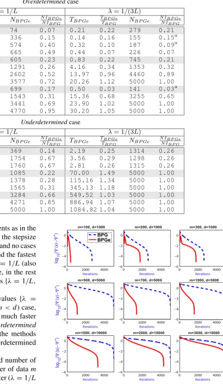
FIGURE 2. Poisson Linear Inverse Problems tests (overdeterminedcase m>d): evolution of the objective function9(xk) vs. iteration number, using the parameter values{λ=1/L, ρ=0.99}and for several problem sizes (measurementsm) with fixed vector dimensiond=100.
In Figure 2, now with the fixed parameter values{λ =
1/L, ρ = 0.99}and for theoverdetermined (m > d) case,
FIGURE 3. Poisson Linear Inverse Problems tests (overdeterminedcase m>d): evolution of the differencek9(xk)−9(x∗)kvs. iteration number,
using the parameter values{λ=1/L, ρ=0.99}and for several problem sizes (measurementsmand vector dimensionsd).
we show the evolution of the objective function9(xk) vs.
iter-ation number and for several problem sizes (measurementsm) with fixed vector dimensiond =100. We observe that always the BPGe algorithm is much faster than the BPG one. In order to observe more clearly the faster convergence, we present in Figure 3 much more simulations but now showing the evolution ofk9(xk)−9(x∗)k. We note that the differences
of both methods are bigger for low dimensiond problems, in fact for the most overdetermined problemsmd.
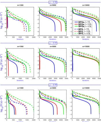
FIGURE 4. Poisson Linear Inverse Problems tests (underdeterminedcase m<d): evolution of the differencek9(xk)−9(x∗)kvs. iteration number,
changing the parameters{λ, ρ}and for several problem sizes (measurementsm) with fixed vector dimensiond=5000.
In theunderdeterminedcase we also analyze the influence of both parameters {λ, ρ} in Figure 4 with respect to the size of the problem (measurementsm) with fixed dimension d =5000. Now, we observe that the value of the parameter ρseems to not affect too much on the global performance of the method, so we will take the valueρ=0.99 when we fix
TABLE 1. Poisson Linear Inverse Problems tests: CPU-time and number of iterations for different cases ofm(number of data) andd(dimension) for two different values of theλparameter foroverdetermined(top) andunderdetermined(bottom) cases.TBPGeandTBPGdenote the CPU-time of BPGe and BPG algorithms, andNBPGeandNBPGthe number of iterations to reach theEXITcriteria. Superscript –a– points out discordant cases related with a fast linear convergence.
the parameter. On the other hand, similar comments as in the overdetermined case can be said with respect to the stepsize parameterλ. Now the behaviour is quite regular, and no cases of very fast convergence have been observed, and the fastest convergence is obtained for the highest valueλ=1/L(also for both algorithms BPGe and BPG). Therefore, in the rest of tests on this paper we fix the parameter values{λ=1/L,
ρ=0.99}.
In Figure 5, now with the fixed parameter values{λ =
1/L, ρ =0.99}and for theunderdetermined(m<d) case, we observe that always the BPGe algorithm is much faster than the BPG one. But, similarly as in the overdetermined case, the differences are bigger when we use the methods for larger ratiosd/m, that is, for the most underdetermined problemsmd.
Finally, in Table1 we give the CPU-time and number of iterations for different sizes of problems (number of datam and dimensiond) for two values of theλparameter (λ=1/L and 1/(3L)) foroverdetermined (top) andunderdetermined (bottom) cases. From the simulations we observe that when the problem has not a very big size (probably because in these other cases longer simulations are needed) the ratios among both methods provide an interesting speed-up, and in most cases theEXITstrategy stops the BPGe algorithm before the maximum number of iterations is reached. On the other hand, we observe that the CPU-time and iteration number ratios are
FIGURE 5. Poisson Linear Inverse Problems tests (underdeterminedcase m<d): evolution of the differencek9(xk)−9(x∗)kvs. iteration number,
using the parameter values{λ=1/L, ρ=0.99}and for several problem sizes (measurementsmand vector dimensionsd).
quite similar, and so there are little differences between them. Note that the BPGe algorithm has an extra step, the line search method of Algorithm 2, but it increments quite a few the final
CPU-time. On the table we have remarked three discordant cases (superscript –a–) related with a fast linear convergence, instead of sublinear. This is illustrated, for example, on the left bottom plot of Figure1(ρ=0.99,m=1000) where the green curve, corresponding toλ = 1/(3L) converges faster than the other colours (as it also occurs in other plots of the same figure). Note that for anoverdetermined problem with random data some initial conditions and data may be led to a faster convergence. For theunderdeterminedproblem there is a regular behaviour in all the simulations.
Therefore, in the Poisson Linear Inverse Problems tests the BPGe algorithm presents a faster performance compared with the BPG algorithm, giving an interesting option for real problems.
B. APPLICATION TO QUADRATIC INVERSE PROBLEMS
In the second test (taken from [8]) we show that BPGe algorithm can deal with a nonconvex Quadratic Inverse Prob-lem (QIP) in which the differentiable term has no globally gradient Lipschitz continuous property. This problem is a natural extension of the linear inverse problem, but now using quadratic measurements. It appears in many popular applica-tions, such as signal recovery [3] and phase retrieve [25] from the knowledge of the amplitude of complex signals.
A general description of the Quadratic Inverse Problem is to find the vectorx∈Rd that solves the system
xTAix'bi, i=1, . . . ,m
being{Ai∈Rd×d|i=1, . . . ,m}a set of symmetric matrices that describes the model, andb=(b1, . . . ,bm)∈Rma vector
of usually noisy measurements.
Following the formalism given in [8, section 5.1], this problem can be formulated as a nonconvex minimization problem as: min ( 9(x):=1 4 m X i=1 (xTAix−bi)2+θg(x):x∈Rd ) , (QIP) whereθ >0 is used to weigh matching the data fidelity crite-ria and its regularizerg. In our experiments, we take a convex l1-norm regularization functiong(x) = kxk1. Note that the
first functionf(x) is a nonconvex differentiable function but that does not admit a global Lipschitz continuous gradient.
The main quality of the BPG and BPGe algorithms (as noted to the BPG in [8]) is that these methods can solve the broad class of problems (QIP). To apply BPG and BPGe on the QIP model properly, we first need to identify a suitable function h (Definition 1). In [8], a proper choice has been given as: h(x)= 1 4kxk 4 2+ 1 2kxk 2 2,
and so now the Bregman distance is given by
Dh(x,y)= {h(x)−h(y)−(kyk2y+y)T(x−y)}.
WhenLis chosen such thatL≥Pm
i=1 3kAik2+ kAik|bi|
then by [8, Lemma 5.1],L-smad condition (Definition 2) holds for the selected functions f(x), g(x) and h(x). Besides, according to the same analysis in [8, Lemma 5.1], we could derive the relative weakly convex parameter as
µ≥Pm
i=1kAik|bi|. In conclusion, we have that:
(i) (f,h) isL-smad,f isµ-relative weakly convex toh. (ii) Assumptions1and2are easily verified.
(iii) f,g,Dh are all semi-algebraic, (see for example [7]).
One can show inductively that HM(x,y) = 9(x) +
MDh(x,y) is semi-algebraic, thus it has KL property
(Definition 4) at any point (x,x). Besides, we could verify that Assumption3holds.
It means, from the convergence SectionIV, that the sequences generated by BPGe algorithm converge to a critical point of the objective function9.
Here, we perform several numerical tests to compare the behaviour of the BPGe and BPG algorithms. As we did with the previous problem (PLIP), we have designed two main families of experiments, considering overdetermined (m> d) andunderdetermined(m < d) cases. To that goal we set different values ofmandd, and we generatemrandom rank-1 matrices Ai = aiaTi in Rd
×d, where the entries of
the vectorsaiare generated following independent Gaussian
distributions with zero mean and unit variance. The accurate x∗ :=arg min{9(x) : x ∈ Rd}is chosen as a sparse vector (the sparsity is 5%) andbi =xTAix∗,i=1, . . . ,m. We set
the weight parameterθ=1 as default.
As a first performance comparison, in Table 2 we give the CPU-time and number of iterations for different sizes of problems (number of datam and dimensiond) for two values of theλ parameter (λ = 1/L and 1/(3L)) for the overdeterminedcase. The valuesTBPGeandTBPGdenote the
CPU-time of BPGe and BPG algorithms, and NBPGe and
NBPG the number of iterations to reach the EXITcriteria,
respectively. From the simulations we observe that the ratios among both methods provide an interesting speed-up, and the EXIT strategy stops the BPGe algorithm before the max-imum number of iterations (kmax = 5000 in this case) is
reached. On the other hand, we observe that the CPU-time and iteration number ratios are quite similar, and so there are little differences between them. Therefore, we note again that although the BPGe algorithm has an extra step (the line search method of Algorithm 2), it increments quite a few the final CPU-time. Also, from the data we observe that although the ratio for the BPGe and BPG algorithms forλ = 1/(3L) is quite good, the option BPGe withλ = 1/L performs many fewer iterations, and so it is the recommended option.
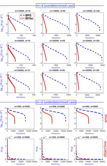
In Figure 6, with the fixed parameter values {λ =
1/L, ρ = 0.99} and for the overdetermined (m > d) andunderdetermined (m < d) cases, we show the evolu-tion ofk9(xk)−9(x∗)k. In this problem we observe that
the performance of the accelerated BPGe algorithm for the overdetermined case is quite good, giving a linear conver-gence. In theunderdetermined case the behaviour seems to
TABLE 2. Quadratic Inverse Problems tests: CPU-time and number of iterations for different cases ofm(number of data) andd(dimension) for two different values of theλparameter for theoverdeterminedcase.TBPGeandTBPGdenote the CPU-time of BPGe and BPG algorithms, andNBPGeand NBPGthe number of iterations to reach theEXITcriteria.
FIGURE 6. Quadratic Inverse Problems tests (overdeterminedcase m>d) and (underdeterminedcasem<d): evolution of the difference k9(xk)−9(x∗)kvs. iteration number, using the parameter values
{λ=1/L, ρ=0.99}and for several problem sizes (measurementsmand vector dimensionsd) and evolution of the objective function9(xk).
be sublinear, and it needs more iterations to reach the desired value (in this simulationskmax = 20000). In both cases the
BPGe algorithms performs much better than the BPG one.
For theunderdetermined case we also show the evolution of the objective function9(xk) vs. iteration number to see
that in this case the objective function takes large values, and therefore, when applying theEXITstrategy the required precision is obtained (a relative error<10−6) giving not too small absolute values.
Therefore, again in the Quadratic Inverse Problems tests the BPGe algorithm presents a faster performance compared with the BPG algorithm, giving an interesting option for real problems.
VI. CONCLUSION
We have introduced a new accelerated Bregman proximal gradient algorithm (BPGe) useful for nonconvex and nons-mooth minimization problems. This algorithm combines two powerful methods to solve large-scale minimization prob-lems. On one hand, we have taken the BPG algorithm [2] able to deal with non-globally Lipschitz continuous gradi-ent problems (firstly defined for the convex case [2] and later extended to the nonconvex case by [8]). And on the other hand, the accelerated extrapolation algorithm (used for instance in the PG algorithm [39]). The use of the Bregman distance paradigm permits to enlarge the number of prob-lems to work with, because we do not need the assump-tion of global Lipschitz gradient continuity. And with the extrapolation technique the convergence of the method is accelerated.
The convergence of the new method is studied, and we have proven that any limit point of the sequence generated by BPGe algorithm is a stationary point of the problem by choosing parameters properly. Besides, assuming Kurdyka-Łojasiewicz property, we have proven the whole sequences generated by BPGe converges to a stationary point.
Finally, we have applied it to two important practical prob-lems that arise in many fundamental applications (and that not satisfy global Lipschitz gradient continuity assumption): Poisson linear inverse problems and quadratic inverse prob-lems, for both,overdetermined andunderdeterminedcases.