Exploring the latent space between brain and behaviour using eigen-decomposition methods

(1)

Exploring the latent space between

brain and behaviour using

eigen-decomposition methods

João André de Matos Monteiro

A dissertation submitted in partial fulfillment of the requirements for the degree of

Doctor of Philosophy

of

University College London.

Department of Computer Science University College London

(2)

(3)

I, João André de Matos Monteiro, confirm that the work presented in this thesis is my own. Where information has been derived from other sources, I confirm that this has been indicated in the work.

(4)

(5)

Abstract

Machine learning methods have been successfully used to analyse neuroimaging data for a variety of applications, including the classification of subjects with different brain disorders. However, most studies still rely on the labelling of the subjects, constraining the study of several brain diseases within a paradigm of pre-defined clinical labels, which have shown to be unreliable in some cases. The lack of understanding regarding the association between brain and behaviour presents itself as an interesting challenge for more exploratory machine learning approaches, which could potentially help in the study of diseases whose clinical labels have shown limitations. The aim of this project is to explore the possibility of using eigen-decomposition approaches to find multivariate associative effects between brain structure and behaviour in an exploratory way.

This thesis addresses a number of issues associated with eigen-decomposition methods, in order to enable their application to investigate brain/behaviour re-lationships in a reliable way. The first contribution was showing the advantages of an alternative matrix deflation approach to be used with Sparse Partial Least Squares (SPLS). The modified SPLS method was later used to model the associations between clinical/demographic data and brain structure, without relying ona priori

assumptions on the sparsity of each data source. A novel multiple hold-out SPLS framework was then proposed, which allowed for the detection of robust multivariate associative effects between brain structure and individual questionnaire items.

The linearity assumption of most machine learning methods used in neuroimag-ing might be a limitation, since these methods will not have enough flexibility to detect non-linear associations. In order to address this issue, a novel Sparse Canon-ical Correlation Analysis (SCCA) method was proposed, which allows one to use sparsity constraints in one data source (e.g. neuroimaging data), with non-linear transformations of the data in the other source (e.g. clinical data).

(6)

(7)

Acknowledgements

Reaching the end of a PhD project is a very long and arduous process, which is only possible with the help of numerous people. In my case, they were far too many to thank them all.

I would like to start by acknowledging my supervisors, Prof. John Shawe-Taylor and Prof. Janaina Mourão-Miranda, whose support and advice were absolutely essential. Without them, this thesis would have never been written.

I would also like to thank my collaborators and colleagues, which helped me throughout the various stages of my PhD: Prof. John Ashburner, Dr. Jessica Schrouff, Dr. Michele Donini, Dr. Dimitrios Athanasakis, Dr. Liana Portugal, Viivi Uurtio, Dr. Jaz Kandola, Dr. Delmiro Fernandez-Reyes, Prof. Juho Rousu, Dr. Gita Prabhu, Dr. Michael Moutoussis, Dr. Gabriel Ziegler, and Martin Axelsen. With a special thank you to Dr. Anil Rao and Dr. Maria João Rosa, who not only were very patient to sit down and answer my questions, but also gave me valuable feedback on the first complete draft of this thesis.

Although not included in this thesis, my work was also comprised of some contributions to the PRoNTo toolbox1. Therefore, I would like to thank the PRoNTo development team for the very insightful discussions: Prof. John Ashburner, Dr. Carlton Chu, Dr. Andre Marquand, Dr. Janaina Mourão-Miranda, Dr. Christophe Phillips, Dr. Jonas Richiardi, Dr. Maria João Rosa, and Dr. Jessica Schrouff.

Working with machine learning methods involves spending a lot of time dealing with all sorts of IT problems, which could not have been solved without the help of the UCL computer science department technical support group. I would like to thank Neil Daeche for handling most of my IT-related issues, and Tristan Clark for keeping the cluster running (probably the most important tool in my project).

1

(8)

I would like to acknowledge the people responsible for collecting and organising the data used in this thesis: the OASIS dataset, and the ADNI dataset. Furthermore, I would like to thank the NSPN consortium for providing their data, even though the results did not make the final version of this thesis.

This project was funded a PhD scholarship awarded by theFundação para a

Ciência e a Tecnologia (SFRH/BD/88345/2012). I would also like to thank the

Wellcome Trust and the Guarantors of Brain, for the extra funding provided to attend several conferences during my project.

On non-work related acknowledgements, I would like to thank all my friends in London, which helped me throughout the years of my PhD. Living in London is definitely not a walk in the park, but it is definitely easier among friends, thus, I would like to specially thank my flatmates Débora Salvado and Florin Rothwell.

Last, but definitely not least, I would like to thank my family for all their continued love and support.

(9)

C.1.1 p-values . . . 181 C.1.2 Distance to constraint . . . 181 C.1.3 ROI variables . . . 183 C.2 SCCA vs. SPLS . . . 184 C.2.1 p-values . . . 184 C.2.2 Hyper-parameter optimisation . . . 185 D Chapter 8 189 D.1 p-values . . . 189 D.2 Hyper-parameter optimisation . . . 190 D.3 Projections . . . 199 Bibliography 200 Glossary 215 13

(14)

(15)

Impact Statement

With the increase in data collection that has been observed in recent years, several datasets are no longer comprised of a single data type coming from a single source, but of different types of data collected from multiple sources. In some situations, one may be interested in modeling the underlying relationships in a dataset containing information coming from two different sources (i.e. views), e.g. neuroimaging data and clinical/demographic data, in order to gain insights into the unobserved latent process which generated the data. This type of modeling has been undertaken in many applications, including: language [Hardoon and Shawe-Taylor, 2011], genetics [Witten et al., 2009, Parkhomenko et al., 2009], neuroimaging [Hardoon et al., 2007], and facial expression recognition [Zheng et al., 2006].

Although, this type of model has applications which span many different fields, the potential medical applications may have a paradigm-shifting impact, by helping redefine the way in which diagnosis is currently carried out, particularly in the psychiatric field. Current diagnostic labels in psychiatry are not very reliable, indeed, they have failed to predict treatment response, which suggests that the labels may not accurately reflect the underlying disease process [Insel et al., 2010]. In order to gain insights into these processes, one has to look at brain diseases from different angles simultaneously, which can be achieved by using eigen-decomposition methods. By making use of more exploratory modeling approaches, one may be able to combine large amounts of heterogeneous data to find patterns which allow for its stratification.

This thesis has provided several contributions to the neuroimaging field, by providing novel ways to model the relationships between brain and behaviour. The first contribution (Chapter 4) showed the advantages of using an alternative matrix deflation approach with sparse eigen-decomposition methods. This approach was then used with a sparse eigen-decomposition method to model the association

(16)

between clinical/demographic features and brain structure without relying ona priori

assumptions regarding the sparsity of each view (Chapter 5). A multiple hold-out framework was then proposed (Chapter 6), which allowed for the detection of robust multivariate associative effects between brain structure and individual questionnaire items. Chapter 7 proposed an adaptation of the Alternating Least Squares (ALS) algorithm, which is a commonly used approach to solve eigen-decomposition problems, this adaptation allowed the ALS to converge more often, while providing comparable results. The ALS was finally adapted to solve a novel eigen-decomposition method (Chapter 8), which allowed one to enforce sparsity in views where the dimensionality is high, while simultaneously exploring non-linear relationships in views where the dimensionality is lower.

The benefits provided by a better understanding of brain disorders goes beyond the realm of academia, it is an essential step to refine current diagnostic tools. This is indeed a very important issue, but a very challenging problem as well, which is why it is unlikely that it will be solved by the work of a single research group. Nevertheless, this thesis has made some contributions which will hopefully enable other researchers to better understand the relationships between brain and behaviour, helping to pave the way for future work which may lead to the improvement of psychiatric diagnosis.

(17)

Publications

Software

• Pattern Recognition for Neuroimaging Toolbox (PRoNTo): http://www.mlnl.

cs.ucl.ac.uk/pronto/

• Sparse Partial Least Squares (SPLS):https://github.com/jmmonteiro/spls

Papers

Submitted / under revision

• J. Schrouff, J. M. Monteiro, L. Portugal, M. J. Rosa, C. Phillips, and J.

Mourão-Miranda. Embedding anatomical or functional knowledge in whole-brain

multiple kernel learning models. Neuroinformatics, (accepted)2

• V. Uurtio, J. M. Monteiro, J. Kandola, J. Shawe-Taylor, D. Fernandez-Reyes, and J. Rousu. A tutorial on canonical correlation methods. ACM Computing

Surveys, (accepted)

• M. J. Rosa, M. Moutoussis, G. Ziegler, J. M. Monteiro, L. Portugal, F. S. Ferreira, E. T. Bullmore, P. Fonagy, I. M. Goodyer, P. B. Jones, the NSPN Con-sortium, R. Dolan, and J. Mourao-Miranda. Brain-behavior modes of covaria-tion in healthy and clinically depressed young people. Scientific Reports, (in preparation)

• M. Donini, J. M. Monteiro, M. Pontil, T. Hahn, A. J. Fallgatter, J. Shawe-Taylor, and J. Mourão-Miranda. Combining heterogeneous data sources for prediction: re-weighting and selecting what is important. NeuroImage, (submitted)

2

(18)

2017

• A. Rao, J. M. Monteiro, and J. Mourão-Miranda. Predictive modelling using neuroimaging data in the presence of confounds. NeuroImage, 2017

2016

• J. M. Monteiro, A. Rao, J. Shawe-Taylor, and J. Mourão-Miranda. A multiple hold-out framework for sparse partial least squares. Journal of Neuroscience

Methods, 271:182–194, 2016

• M. Donini, J. M. Monteiro, M. Pontil, J. Shawe-Taylor, and J. Mourao-Miranda. A multimodal multiple kernel learning approach to Alzheimer’s disease

detec-tion. In Machine Learning for Signal Processing (MLSP), 2016 IEEE 26th

International Workshop on, pages 1–6. IEEE, 2016

• A. Rao, J. Monteiro, and J. Mourao-Miranda. Prediction of clinical scores from neuroimaging data with censored likelihood Gaussian processes. In Pattern

Recognition in Neuroimaging (PRNI), 2016 International Workshop on, pages

1–4. IEEE, 2016

2015

• J. M. Monteiro, A. Rao, J. Ashburner, J. Shawe-Taylor, and J. Mourão Miranda. Multivariate effect ranking via adaptive sparse PLS. InPattern Recognition in

NeuroImaging (PRNI), 2015 International Workshop on, pages 25–28. IEEE,

2015

• A. Rao, J. M. Monteiro, J. Ashburner, L. Portugal, O. Fernandes, L. De Oliveira, M. Pereira, and J. Mourão-Miranda. A comparison of strategies for incorpo-rating nuisance variables into predictive neuroimaging models. In Pattern

Recognition in NeuroImaging (PRNI), 2015 International Workshop on, pages

61–64. IEEE, 2015

2014

• J. M. Monteiro, A. Rao, J. Ashburner, J. Shawe-Taylor, and J. Mourão-Miranda. Leveraging clinical data to enhance localization of brain atrophy. In

Interna-tional Workshop on Machine Learning and Interpretation in Neuroimaging,

pages 60–68. Springer, 2014

(19)

List of Figures

2.1 Example of a linear regression. . . 37

2.2 Mapping a dataset into a higher dimensional feature space. . . 39

2.3 Single train/test data split scheme. . . 45

2.4 k-fold cross-validation scheme. . . 46

2.5 Three-way split validation scheme. . . 47

2.6 Nested cross-validation scheme. . . 48

3.1 Principal Component Analysis (PCA) . . . 55

4.2 First three image weight vectors computed using each deflation step. 81 4.3 First three clinical weight vectors computed using each deflation step. 82 4.4 Projections of the data matrices onto the weight vectors computed using both deflation strategies. . . 83

5.1 Clinical weight vectors. . . 90

5.2 Image weight vectors. . . 90

6.1 Hyper-parameter optimisation framework. . . 98

6.2 Permutation framework. . . 100

6.3 Average absolute correlation on the hold-out datasets. . . 106

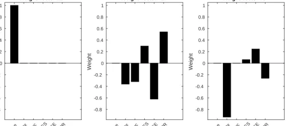
6.4 SPLS clinical weight vectors. . . 107

6.5 SPLS image weight vectors. . . 108

6.6 Projection of the data onto the SPLS weight vector pairs. . . 110

7.1 Average correlations for both datasets. . . 126

7.2 Average test correlations for each hyper-parameter optimisation step. Original dataset ({X,Y}). . . 128

(20)

7.3 Average test correlations for each hyper-parameter optimisation step.

Noisy dataset ({X0,Y0}). . . 129

7.4 Mean ROI weight vectors across the 10 hold-out splits. . . 130

7.5 Mean clinical weight vectors across the 10 hold-out splits. . . 131

7.6 Comparison of ALS algorithms using original dataset{X,Y}. . . 132

7.7 Comparison of ALS algorithms using dataset with added noise{X0,Y0}.133 7.8 Average of the optimal test correlations for all the seven methods tested.140 7.9 Average test correlations for each hyper-parameter optimisation step, using SPLS-PM. . . 141

7.10 Average test correlations for each hyper-parameter optimisation step, using SPLS-ALS-EN. . . 142

7.11 Properties of features selected inX by each one of the methods tested.144 7.12 Correlation matrices between the variables selected by the averageu and v for the non-sparse methods. . . 145

7.13 Correlation matrices between the variables selected by the averageu and v for the SCCA methods. . . 146

7.14 Correlation matrices between the variables selected by the averageu and v for the SPLS methods. . . 147

7.15 Data projected onto the best weight vector pair for each one of the non-sparse methods tested. . . 148

7.16 Data projected onto the best weight vector pair for each one of the SCCA methods tested. . . 149

7.17 Data projected onto the best weight vector pair for each one of the SPLS methods tested. . . 150

8.1 Average optimal test correlation across the 10 different data splits. . 159

8.2 Projections of the subjects onto the weight vectors computed using non-sparse methods. . . 160

8.3 Projections of the subjects onto the primal-dual SCCA weight vectors. 161 8.4 Subject conversion from MCI to AD after 6 months. . . 162

(21)

B.1 Mean absolute correlation value computed for each split of the data for the first weight vector pair during the hyper-parameter optimisation step. . . 173 B.2 Mean absolute correlation value computed for each split of the data for

the second weight vector pair during the hyper-parameter optimisation step, using projection deflation. . . 174 B.3 Mean absolute correlation value computed for each split of the data for

the second weight vector pair during the hyper-parameter optimisation step, using PLS Mode-A deflation. . . 175 B.4 Mean of clinical weight vector using PLS. . . 176 B.5 Mean of image weight vectors using PLS. . . 176 B.6 Mean of second SPLS clinical weight vectors using projection deflation

and PLS Mode-A deflation. . . 177 B.7 Mean of second SPLS image weight vectors using projection deflation

and PLS Mode-A deflation. . . 178 B.8 Projection of the data onto the SPLS weight vector pairs. . . 179

C.1 Relative distances to the constraints. . . 182 C.2 Average test correlations for each hyper-parameter optimisation step,

using SPLS-ALS-L1. . . 185 C.3 Average test correlations for each hyper-parameter optimisation step,

using SCCA-ALS-L1. . . 186 C.4 Average test correlations for each hyper-parameter optimisation step,

using SCCA-ALS-EN. . . 187

D.1 Average test correlations for each hyper-parameter optimisation step, using SCCA-LK-LK. . . 190 D.2 Average test correlations for each hyper-parameter optimisation step,

using SCCA-PK-PK. . . 191 D.3 Average test correlations for each hyper-parameter optimisation step,

using SCCA-GK-GK. . . 192 D.4 Average test correlations for each hyper-parameter optimisation step,

using SCCA-L1-LK. . . 193 21

(22)

D.5 Average test correlations for each hyper-parameter optimisation step, using SCCA-L1-PK. . . 194 D.6 Average test correlations for each hyper-parameter optimisation step,

using SCCA-L1-GK. . . 195 D.7 Average test correlations for each hyper-parameter optimisation step,

using SCCA-LK-L1. . . 196 D.8 Average test correlations for each hyper-parameter optimisation step,

using SCCA-PK-L1. . . 197 D.9 Average test correlations for each hyper-parameter optimisation step,

using SCCA-GK-L1. . . 198 D.10 Subject conversion from MCI to AD after 6 months, using non-sparse

methods. . . 199

(23)

List of Tables

5.1 Optimal sparsity hyper-parameters per weight vector pair. . . 89 6.1 Demographic information of the dataset. . . 103 6.2 PLS p-values computed with 10 000 permutations. . . 105 6.3 SPLSp-values computed with 10 000 permutations. . . 105 6.4 Top 10 atlas regions for the first image weight vector. . . 109 6.5 Top 10 atlas regions for the second image weight vector. . . 109 7.1 Demographic information of the dataset. . . 124 B.1 MMSE questions/tasks. . . 171 B.2 Atlas regions for the first image weight map. . . 178 B.3 Atlas regions for the second image weight map. . . 179 C.1 Correlations on the 10 hold-out sets, with the corresponding p-values. 181 C.2 Complete list of ROI volumes used as features in X. . . 183 C.3 Correlations on the 10 hold-out sets for the non-sparse methods, with

the correspondingp-values. . . 184 C.4 Correlations on the 10 hold-out sets for the sparse methods, with the

correspondingp-values. . . 184

D.1 Correlations on the 10 hold-out sets using the KCCA methods, with the correspondingp-values in parenthesis. . . 189 D.2 Correlations on the 10 hold-out sets using the primal-dual SCCA

(24)

(25)

Nomenclature

Greek Symbols

δ Step size of SCCA-ALS (Chapter 8)

γ Regularisation hyper-parameter

λ Eigenvalue

ω Projection ofY onto v, i.e. ω=Y v

ξ Projection ofX onto u, i.e. ξ=Xu

Matrices and vectors

Cxx Covariance matrix of X

Cxy Covariance matrix of X and Y

Cyy Covariance matrix of Y

Kx Kernel ofX

Ky Kernel ofY

w(i) Vector wat the ith iteration.

X(:, j) jth column of X, wherej∈ {1, . . . , p} X(i,:) ith row ofX, wherei∈ {1, . . . , n}

X| Transpose of matrixX

X Data matrix withn rows andp columns

(26)

Other variables

cu andcv SPLS hyper-parameters

d Singular value

n Number of samples

p and q Number of features

(27)

Abbreviations

AD Alzheimer’s Disease

ADAS Alzheimer’s Disease Assessment Scale

ALS Alternating Least Squares

CCA Canonical Correlation Analysis

CDR Clinical Dementia Rating

CSF Cerebrospinal Fluid

CV Cross-Validation

DTI Diffusion Tensor Imaging

FAQ Functional Assessment Questionnaire

fMRI Functional Magnetic Resonance Imaging

FTD Frontotemporal Dementia

FWHM Full Width at Half Maximum

GM Grey Matter

KCCA Kernel Canonical Correlation Analysis

KRR Kernel Ridge Regression

LASSO Least Absolute Shrinkage and Selection Operator

(28)

MMSE Mini-Mental State Examination

MRI Magnetic Resonance Imaging

MSE Mean Squared Error

PCA Principal Component Analysis

PLS Partial Least Squares

PLSR Partial Least Squares Regression

RAVALT Rey Auditory Verbal Learning Test

ROI Region Of Interest

SCCA Sparse Canonical Correlation Analysis

SES Socioeconomic Status

SNP Single Nucleotide Polymorphism

SPLS Sparse Partial Least Squares

SPLS-DA Sparse Partial Least Squares Discrimination Analysis

SPM Statistical Parametric Map

SVD Singular Value Decomposition

VBM Voxel-Based Morphometry

WM White Matter

(29)

Chapter 1 Introduction

1.1 Neuroimaging and machine learning

For many years, one of the main limitations when studying the human brain was the fact that acquiringin vivo data was only possible using very invasive procedures (e.g. electro-physiological recordings). The introduction of neuroimaging techniques, such as Magnetic Resonance Imaging (MRI), drastically changed the field, by making it possible to acquirein vivo brain images in a non-invasive way.

MRI allows the acquisition of 3D brain images by using the magnetic properties of the atoms in the body, more specifically, the hydrogen nuclei in the water molecules. These images are comprised of many voxels, where each voxel can be seen as a pixel in a 3D space, i.e. whereas a pixel is a 2D square containing information about a small region of a 2D image, a voxel is a 3D cube containing information about the signal in a small region of a magnetic resonance (MR) image. Depending on the particular MRI acquisition sequence, different types of images can be obtained. One of the most commonly used types of structural MR images is the T1-weighted image, due to the fact that it provides a reasonable contrast between the different brain tissues, more specifically, between Grey Matter (GM) and White Matter (WM), and between GM and Cerebrospinal Fluid (CSF) [Chu, 2009].

The raw images provided by the MRI scanners cannot be directly used to perform a statistical analysis, as the MR signal intensities and brain shapes will be different between the images coming from different subjects. Therefore, structural MR images are subjected to a pre-processing pipeline before they are analysed, which is usually comprised of three main steps: segmentation, normalisation, and smoothing [Ashburner and Friston, 2005]. The segmentation step is applied to identify

(30)

30 Chapter 1. Introduction

the different types of tissue in the brain and create separate images based on the probability of each voxel corresponding to a particular tissue (e.g. GM, WM, CSF), this is done in order to normalise the values of each pixel to a range between 0 and 1 [Chu, 2009], enabling comparisons across different MR images. These probability maps are then normalised to a standard brain template, so that brains from different subjects, which have different shapes, can be analysed together. Finally, the images are usually subjected to a final spatial smoothing step, in order to remove some of the higher spatial frequency signal, which is usually associated with noise [Chu, 2009]. This smoothing is performed by performing a convolution between the images and a Gaussian kernel with a pre-determined Full Width at Half Maximum (FWHM), essentially “blurring” the images.

One of the most common ways to analyse structural differences in the pre-processed MR images is by using Voxel-Based Morphometry (VBM) [Ashburner and Friston, 2000], which allows one to determine which specific voxels in the brain are significantly correlated with the variable that is being tested, by performing a statistical test on each individual voxel. Although VBM is still very popular in neuroscience, it is an univariate approach, which means that each voxel is tested individually, without taking into account the interaction between all the voxels. In order to model this interaction, one has to use multivariate approaches, such as

machine learning methods. These methods change the question that VBM tries to

answer; instead of estimating which voxels are individually correlated with the effect, machine learning methods look for general patterns in the data which allow one to perform several tasks, including: classifying the subjects as belonging to a particular class (e.g. diseased subjects vs. healthy subjects), predicting a clinical/demographic score (e.g. age), gaining novel insights by finding associations between different types of data (MRI scans and clinical/demographic scores), etc.

Machine learning methods have been successfully used to analyse neuroimaging data for a variety of applications, including the study of neurological and psychiatric diseases. So far, however, most of these studies have focused on supervised binary classification problems, i.e. they attempt to summarise clinical assessment into a single measure (e.g. diagnostic classification) and the output of the models is limited to a probability value and, in most cases, a binary decision (e.g. healthy

(31)

1.2. Outline and contributions 31

vs. patient) [Ecker et al., 2010, Mourão-Miranda et al., 2005, Nouretdinov et al., 2011, Orrù et al., 2012, Rao et al., 2011, Klöppel et al., 2008]. This paradigm may present itself as a limitation when studying brain diseases whose underlying disease process is not yet completely understood and, therefore, might have an unreliable categorical classification. Indeed, this is a well known problem in psychiatry [Insel et al., 2010], where insights regarding the associations between brain and behaviour are still limited.

The lack of understanding regarding the associations between brain and be-haviour presents itself as an interesting challenge for more exploratory machine learning approaches, such as eigen-decomposition methods, including several variants of Canonical Correlation Analysis (CCA) and Partial Least Squares (PLS). These methods can model the associations between brain and behaviour, by finding a latent subspace where these associations are the strongest.

1.2 Outline and contributions

The aim of this thesis is to explore the possibility of using eigen-decomposition approaches to find multivariate associative effects between brain structure and behaviour. Several variants of these methods will be tested, including versions that allow for sparse and non-linear solutions. As a proof of concept, all the methods explored in this thesis used dementia datasets, as the relationships between brain regions and behaviour are better understood in dementia, allowing for more reliable comparisons with previous studies.

The thesis is laid out as follows:

• Chapter 2 will introduce some basic machine learning concepts, with an em-phasis on supervised learning. It will conclude with some remarks regarding the limitations of these methods, and the motivation for exploring the use of eigen-decomposition methods in this thesis.

• Chapter 3 will describe some of the most relevant eigen-decomposition methods used in this thesis. It will serve as a general introduction and review of these methods, before presenting the main contributions of this thesis in the following chapters.

(32)

32 Chapter 1. Introduction

Partial Least Squares (SPLS), which tries to address a limitation of the deflation approach originally proposed by Witten et al. [2009]. Publication associated with the chapter: Monteiro et al. [2014].

• Chapter 5 describes an alternative permutation based framework to optimise the SPLS hyper-parameters, along with an earlier application of SPLS to dementia using different levels of sparsity for both neuroimaging and clinical/demographic data. Publication associated with the chapter: Monteiro et al. [2015].

• Chapter 6 takes the type of analysis performed in Chapter 5 a step further. In this chapter, a multiple-holdout framework is proposed, which is able to find robust multivariate associations between brain and behaviour. The framework was applied to a novel experimental setup, using whole-brain structural MRI data and individual items from a clinical questionnaire. This experimental setup allowed us to find multivariate associations between a subset of brain voxels, and a subset of the individual questionnaire items, which was not previously shown in the literature. Addition comparisons regarding the influence of the sparsity constraints and the influence of the matrix deflation step were also made. Publication associated with the chapter: Monteiro et al. [2016]. • Chapter 7 presents the background for Chapter 8. It proposes an adaptation

of the Alternating Least Squares (ALS) algorithm to solve several Sparse CCA (SCCA) and SPLS optimisation problems. It also compares seven different eigen-decomposition methods, some of these comparisons have not been previously made in the literature.

• Chapter 8 proposes a novel primal-dual SCCA method. This method allows one to model the multivariate associations between brain and behaviour by using both sparsity constraints, and non-linear transformations of the data. • Chapter 9 provides a general summary of the conclusions of this thesis, along

(33)

Chapter 2 Pattern analysis

The automatic detection of patterns in a dataset is an essential part of solving machine learning problems. These patterns are defined as any relations, regularities or structure that can be used to extract any meaningful information from the data [Shawe-Taylor and Cristianini, 2004]. In order to detect these patterns, a number of examples must be provided to a machine learning method. These examples are calledsamples, which can be represented as vectors with a certaindimension.

To illustrate these concepts, consider a dataset of whole-brain structural MRI scans from 100 patients which will be used as input to a machine learning method. The number of samples is equal to the number of subjects (n= 100) and the dimension of each sample is equal to the number offeatures. In this case, each feature corresponds to a voxel in the image, i.e. if the number of voxels is 100 000, then each sample lies on a 100 000 dimensional space: xi∈R1×100000, i∈ {1, . . . , n}. The dataset can be organised in adata matrix X ∈Rn×p, where n is the number of samples, p is the number of features, and each row ofX corresponds to a samplexi.

The information contained in the data matrixX can be used for many different tasks. The type of machine learning method used depends on the task at hand. In neuroimaging, the most popular machine learning methods belong to two main types: supervised learning and unsupervised learning.

Supervised learning methods are used when one is trying to predict a value

yi associated with an example xi, i.e. these methods try to answer the following

question: “Given an example xi, what is its associatedyi?”. The type of supervised

learning method used to answer this question will depend on the nature of what one is trying to predict (yi), thus, supervised learning problems are sub-divided into

(34)

34 Chapter 2. Pattern analysis

two main categories: classification and regression. The former deals with cases in which the aim is to predict whether an example belongs to a certain pre-defined class (e.g. healthy vs. diseased), while the latter deals with cases in which the aim is to predict a continuous score (e.g. age). Therefore, in a classification setting, yi will

be an integer number which denotes the label of xi (e.g. yi= 0: healthy vs.yi= 1:

diseased), whereas in a regression settingyi will be a continuous value which denotes

thetarget that one is trying to predict (e.g. age).

Unsupervised learning focuses on trying to find patterns in the data without any concern for labels or targets. These are normally used as exploratory approaches to find structure in the data which can then be used for several tasks, including data compression, data visualisation, clustering, or even as a step for further analysis using supervised learning.

The aim of this chapter is to make an overview of some of the general machine learning concepts, with an emphasis on supervised learning (Sections 2.1 to 2.2.3). The chapter will conclude with a few examples of applications of supervised learning methods in the neuroimaging literature, and some considerations regarding their general limitations when applied to clinical problems in neuroimaging (Section 2.3). In an attempt to address some of these limitations, this project has used more exploratory machine learning approaches, which shall be presented in Chapter 3.

2.1 Model training

Some of the concepts presented in this chapter are applicable in both supervised and unsupervised learning settings. However, in order to keep the introduction to a reasonable size, the examples will be given in a supervised learning setting. More specifically, in a regression setting, as some of the concepts associated with regression problems will be important for Chapters 7 and 8.

Let X ∈_Rn×p _{be a data matrix containing} _n _{samples with} _p _{features (with}

n > p), and y∈Rn×1 be a vector with the targets associated with each sample. In a supervised learning setting, the aim is to find a function f that maps each input

xi∈X to each output yi ∈y. The trivial solution to this problem would be to

make an exact map of each input to its corresponding target (f(xi) =yi∀ {1, . . . , n}).

However, one also wishes to makef a general function that can handle samples x0

(35)

2.1. Model training 35

f which, given a new example x0, makes a reasonable prediction of its target y0:

f : X →y

f : x0→y0

The distance between the values given byf(X) and the actual targetsyis given by theloss function L. The optimal functionf will be the one which minimises the loss:

f = arg min

f

L(f,y) (2.1)

In some settings, one may train a modelf which perfectly fits the data (f(xi) =

yi∀i∈ {1, . . . , n}) while providing poor predictions for new examples x0. In these

cases, it is said that the model f is too complex and itoverfits the data. One of the ways to avoid these scenarios, is by penalising solutions of f which are too complex, thus, an extra penalty function P is added to Equation 2.1. The loss function (L) plus the penalty function (P) will constitute theobjective function J that one tries to minimise: f = arg min f J(f,y) ⇔ f = arg min f L(f,y) +γP(f) (2.2)

where γ is thehyper-parameter of the model, which controls the trade-off between the loss and the penalty.

In general, more complex functionsf lead to lower losses L, which decrease the cost J (Equation 2.2). However, the penalty termP increases with the complexity of f, which results in the increase of J. Therefore, in order to minimise J, there must be a compromise between the loss and the complexity. Note that if the penalty hyper-parameterγ is too small, the complexity of f will be too high, and the model will overfit. However, if γ is too large, then f will not have enough complexity to properly model the data, and the model f will underfit.

There have been several loss functions (L) and penalty functions (P) proposed in the literature, which contain different properties, leading to different solutions. In order to better illustrate these concepts, a regression example is provided below.

(36)

2.1.1 Linear regression

Consider a case in which one wishes to find a functionf that uses the information from a sample vector xi∈X to predict a continuous target variableyi. One of the

ways to solve this problem is by using a model called linear regression. This model uses a loss function known as the squared loss:

L=

n

X

i=1

(yi−f(xi))2 (2.3)

Since the model is linear, this implies that f is a linear function, thus, the predictions provided by f consist of a weighted linear combination of the input features: f(x) = p X j=1 (xjwj) +b (2.4)

where wj are known as theweights, and b is known as thebias term.

If the targetsy and the features ofX are mean-centered, i.e. the mean of the targetsy is equal to zero and the mean of each column ofX is equal to zero, then

b= 0 and Equation 2.4 can be re-written as:

f(x) =xw

where w∈_Rp×1 _{is known as the}_{weight vector}_{. By writing the problem using matrix}

notation, the squared loss (Equation 2.3) can be re-written as:

L(X,y,w) =ky−Xwk2₂

where k · k2 denotes thel2-norm (also known as the Euclidean norm).

In its simplest version, linear regression does not contain a penalty term, therefore, the objective function will be equal to the loss function, i.e.J =L. In order to find the minimum of the objective functionJ, one has to find the weight vectorw which makes the function f model the data with the smallest possible loss. The problem can thus be written as the following optimisation problem:

w= arg min

w J

(X,y,w) ⇔ w= arg min

w

(37)

The optimisation problem expressed in Equation 2.5 can be re-written as:

J(X,y,w) = (y−Xw)|(y−Xw) (2.6)

which can then be differentiated to calculate its minimum [Shawe-Taylor and Cris-tianini, 2004]: ∂J ∂w=0 −2X|y+ 2X|Xw=0 X|Xw=X|y w= (X|X)−1X|y (2.7)

Ifp= 1, then the solution will be a line whose fit minimises the squared distance betweenyi andf(xi), an example can be seen in Figure 2.1. For higher dimensional

problems (p >1), the solution given bywwill correspond to a hyperplane.

-1.5 -1 -0.5 0 0.5 1 1.5 x -1.5 -1 -0.5 0 0.5 1 1.5 2 y Data Linear fit

Figure 2.1: Example of a linear regression.

The solution to the optimisation problem expressed in Equation 2.5 may overfit the data, thus, it is often desirable to add a penalty term. This is especially true if

p > n, which is known as an ill-conditioned problem, where the optimisation problem will not have an unique solution.

There are several types of penalties that can be chosen, which will result in different solutions for w. One of these is thel2-norm penalty (P(w) =kwk22), also

(38)

known as theridge penalty. By using this penalty, one has to re-write the problem expressed in Equation 2.5 as:

w= arg min

w

ky−Xwk2₂+γkwk2₂ (2.8)

Following the same procedure used to derive Equation 2.7, one obtains the following solution:

w= (X|X+γI)−1X|y

where I∈_Rp×p _{is an identity matrix.}

The ridge penalty provides solutions forwin which all the features are included in the model, and the ones that are not informative are down-weighted. However, in some cases, it might be desirable to obtain asparsesolution, i.e. a solution where the contribution of certain features is set to zero (wj = 0). These approaches perform

feature selection, which is a desirable property to have if only a subset of the features

contains relevant information, since non-informative features are excluded from the model.

One of the most popular sparse penalty functions is the l1-norm penalty. When

used in a regression setting, it gives rise to the popular method known as Least Absolute Shrinkage and Selection Operator (LASSO) [Tibshirani, 1996]:

w= arg min

w

ky−Xwk2₂+γkwk1 (2.9)

Despite the popularity of the LASSO, one of its disadvantages is that it tends to exclude variables which are correlated with other variables already included in the model, e.g. if featurex1 is correlated with feature x2, the tendency is for only

one of the features to be included: w16= 0, w2= 0; or w1= 0, w26= 0. This may lead

to informative features being excluded from the model, based solely on the fact they are correlated with other informative features. In order to address this issue, Zou and Hastie [2005] proposed an approach known as theelastic net, which consists in adding an extral2-norm penalty to the LASSO optimisation problem, resulting in a

(39)

method that provides sparse solutions while maintain a grouping effect:

w= arg min

w

ky−Xwk2₂+γ1kwk1+γ2kwk22

whereγ1andγ2denote the hyper-parameters that control the influence of thel1-norm

and l2-norm penalties, respectively.

The description of the algorithms available to solve the LASSO and elastic net optimisation problems is beyond of the scope of this thesis, for more details, please refer to the papers by Efron et al. [2004] and Friedman et al. [2010].

2.1.2 Kernel methods

So far, all the methods presented were linear methods, i.e. the solution consists of a linear combination of the features, which is expressed by the weight vector. However, sometimes the patterns of interest in the data are non-linear. This means that linear methods may not be able to estimate a model f which is able to predict well the labels/targetsy0 for new data points x0. One of the ways to address these situations is by mapping the data in the original input space into a higher dimensional space, where the problem is linearly solvable.

Consider the classification example on the left hand side of Figure 2.2. In this case, the aim is to classify the two groups of data points (red and blue) by finding a function f which defines a boundary separating the two groups. As one can see, it is impossible to do this with a linear function, i.e. there is no straight line which is able to separate the two groups (Figure 2.2 - left). However, if a new variable is introduced

x3=x21+x22, then the groups are linearly separable using a plane (Figure 2.2 - right).

Figure 2.2: Mapping a dataset into a higher dimensional feature space. A new feature

(40)

Performing this mapping can be done explicitly, by introducing new features (Figure 2.2), or done implicitly, by using a kernel.

This section will give a brief overview of some of the properties of kernels, and how they can be used in machine learning methods.

2.1.2.1 Kernels

In order to understand how kernels are constructed, consider an hypothetical input vectorx∈_Rp_{, and a function} _φ_{that maps this vector into a feature space} _F_⊆

RP, where P>p:

φ:x∈_Rp7→φ(x)∈F ⊆_RP

A kernel function takes two input vectorsxi,xj∈X, maps them into a higher

dimensional feature space and performs the dot product between the two:

κ(xi,xj) =hφ(xi), φ(xj)i

The results are then stored in akernel matrix (also known as a kernel):

K=       κ(x1,x1) · · · κ(x1,xn) .. . . .. ... κ(xn,x1) · · · κ(xn,xn)      

Thus, the kernel can be seen as a matrix containing information about how closexi

is toxj in the feature spaceF.

The type of kernel depends on the transformation φ(·) that the samples are subjected to. If a linear kernel is used, then no transformation is performed on the input vectors prior to the dot product (φ(x) =x). Thus, the kernel function will simply be the dot product of the arguments:

κ(xi,xj) =hxi,xji

In this case, the results will be equivalent to running the machine learning method in the original input space [Shawe-Taylor and Cristianini, 2004]. The kernel can be

(41)

computed by multiplying the input data matrix with its transpose:

K=XX| (2.10)

This will provide some computational advantages for cases in whichpn, due to the fact that one will work with the kernel matrix K∈_Rn×n_{, instead of the larger}

data matrixX ∈_Rn×p_{. However, this is not the main strength of kernel methods.}

The main reason why these methods are popular, is due to a property known as

the kernel trick, which allows one to obtain a mapping into a higher dimensional

feature spaceF without explicitly performing the mapping φ(·) in the original input space. This can be done by computing the kernelK using (2.10) and then applying a transformation on K.

Some of the more popular types of non-linear kernels include the polynomial kernel (κd) and the Gaussian kernel (κG):

κd(xi,xj) = (hxi,xji+R)d and κG(xi,xj) = exp _hx i,xji σ2 − hxi,xii 2σ2 − hxj,xji 2σ2 (2.11)

where d is the degree of the polynomial kernel, R is a hyper-parameter which

controls the influence of the linear terms for the polynomial kernel, and σ is an hyper-parameter which controls the flexibility of the Gaussian kernel [Shawe-Taylor and Cristianini, 2004].

Note that the kernel matrixKcontains all the information necessary to compute the distance between two vectors. However, some information is lost when the input matrixX is converted to K, namely, the orientation of the dataset with respect to the origin [Shawe-Taylor and Cristianini, 2004]. In order to make the concept of the kernel trick clearer, an example is provided below.

Example: Non-linear mapping using a polynomial kernel

Let X ∈Rn×p denote a data matrix with n samples and p features. For a low dimensional problem (e.g. p= 2), if one would want to include all the possible

(42)

combinations of polynomials of degree 2, one could perform the following mapping:

φ(x) = [x2₁, x₂2,√2x1x2,

√

2Rx1,

√

2Rx2, R] (2.12)

As mentioned previously (Equation 2.11), the term R controls the contribution of the linear terms, i.e. the larger it is, the stronger the influence of the linear terms is, which should help prevent overfitting.

As one can see in Equation 2.12, this mapping increased the number of variables. However, one could use a kernel instead, which avoids performing this explicit mapping.

Let x and z be two row vectors from matrix X (i.e. two samples from the

dataset). The dot product betweenhφ(x), φ(z)i is equivalent to:

hφ(x), φ(z)i= (hx,zi+R)d

The proof for this equivalence is done by expanding the polynomial kernel κd

(Equation 2.11) using the binomial theorem [Shawe-Taylor and Cristianini, 2004]:

κd(x,z) = (hx,zi+R)d= d X s=0 d s ! Rd−shx,zis= = 2 0 ! R2hx,zi0+ 2 1 ! R1hx,zi1+ 2 2 ! R0hx,zi2 =R2+ 2Rhx,zi+hx,zi2 =R2+ 2R(x1z1+x2z2) + (x1z1+x2z2)2 =R2+ 2Rx1z1+ 2Rx2z2+x21z12+ 2x1z1x2z2+x22z22 (2.13)

Note that performing the explicit mapping ofxand z using Equation 2.12, and then performing the dot product (hφ(x), φ(z)i) will lead to the same expression in the last line of Equation 2.13, therefore, both operations are equivalent. However, using the kernel trick is much more efficient, as the number of non-linear features will grow very large with the number of features in X and the degree of the polynomial.

A kernel method is essentially a machine learning method which takes kernels

K as inputs, instead of the original data matrices X. The algorithms used in kernel methods work with different types of kernels, making the methods more

(43)

modular [Shawe-Taylor and Cristianini, 2004], i.e. one can use different types of linear and non-linear models simply by swapping the kernel that is used. In order to illustrate some of the concepts associated with kernel methods, the adaptation of ridge regression (Equation 2.8) into its kernel formulation is presented below.

2.1.2.2 Kernel Ridge Regression (KRR)

The ridge regression problem expressed in Equation 2.8 can be adapted to be solved using kernels. The first step is to write the objective function in matrix notation (similar to Equation 2.6):

J(X,y,w) = (y−Xw)|(y−Xw) +γw|w

Then, the problem is transformed from its primal representation, into its dual

representation, by representing the weight vectorswas a combination of the training

samples,w=X|α:

J(X,y,α) = (y−XX|α)|(y−XX|α) +γα|XX|α (2.14)

By using Equation 2.10, one can re-write Equation 2.14 as:

J(K,y,α) =y|y−y|Kα−α|Ky+α|K2α+γα|Kα (2.15) This in turn can be differentiated with respect to α and set to0, in order to find its minimum: ∂J ∂α =0 0−Ky−Ky+ 2K2α+ 2γKα=0 −2Ky+ 2K(K+γI)α=0 α= (K+γI)−1y

where I∈_Rn×n _{is an identity matrix.}

This method is known as the Kernel Ridge Regression (KRR), it has adual

solution, given by α, which is referred to as a dual variable [Shawe-Taylor and

(44)

(as described in Section 2.1.1) ifK corresponds to a linear kernel. In this case, the

primal variable wcan be recovered using the dual variableα, i.e.w=X|α.

As previously mentioned, one of the advantages of kernel methods is thatK

can be non-linear, which means that the optimisation problem will be equivalent to solving a ridge regression problem in a non-linear, higher dimensional feature spaceF. This may provide better results, if the patterns that one is trying to detect are non-linear. However, it may lead to overfitting, and moreover, it will not be straightforward to recover the weights win the original input space.

2.2 Model validation

As mentioned in Section 2.1, when training a supervised machine learning model, the main goal is to find a functionf which, given a new samplex0, is able to make a reasonable prediction of its corresponding label/targety0. In order to check if the training was successful, the ability of the model to generalise for new data should be assessed, i.e. one should validate the model. For a classification problem, this can be formulated as the following question: “Given a new set of data {X0,y0}with N new samples, how many samples does the modelf correctly classify?”. More specifically, one wants to determine the fraction of timesf(x0_i) =y_i0. This metric is known as the

accuracy of the model.

In the case of a regression problem, the question one is trying to answer is: “Given a new set of data {X0,y0} with N new samples, how large is the distance

between the predictions f(x0_i) and the true targets y_i0?”. More specifically, one is interested in quantifying the error that the model f makes when predicting the targets y0. One of the most commonly used metrics to quantify this error is the Mean Squared Error (MSE):

MSE = 1 N N X i=1 (y_i0−f(x0_i))2

The strategies used for validation will depend not only on the research question, but also on the model itself and the amount of data available. One of the main factors which influences the choice in validation strategy is the existence of hyper-parameters that have to be optimised.

(45)

2.2. Model validation 45

without hyper-parameter optimisation) will be made in the following sections.

2.2.1 Validation without hyper-parameter optimisation

A hyper-parameter will be defined as any term which controls the complexity of a model. For example, this could be the penalty hyper-parameter γ (as defined in Equation 2.2), or an hyper-parameter which controls the complexity of a kernel, i.e. thedhyper-parameter for polynomial kernels, or theσhyper-parameter for Gaussian kernels (as described in Equation 2.11).

Letf be a model without hyper-parameters (or with hyper-parameter values fixeda priori) that one wishes to validate, the simplest ways to validate a model, is simply to take all the available data and split it into a train set and a test set (Figure 2.3). The modelf is then trained using the train data, and the test data is

used to compute the performance metric (e.g. accuracy, MSE, etc.).

Test

Train

Figure 2.3: Single train/test data split scheme.

This approach will usually work well if the dataset has a large number of samples. However, if this is not the case, then the estimated model may not be able to achieve a good performance, since it will be trained using a very small dataset. Moreover, the estimation of the model’s performance may be very different from the “true” performance, since a very small dataset is used to estimate it.

The datasets available in neuroimaging usually do not contain enough samples to justify using the approach described in Figure 2.3. One of the most common ways to address this issue is to use an approach known as k-fold Cross-Validation (k-fold CV). The process is illustrated in Figure 2.4, which starts by splitting the data intoknon-overlapping sets with the same size. For the first fold (k= 1) the set

kis left out of the dataset ({Xk,yk}) and the model is trained with the remaining

data ({X₍₋_k₎,y₍−k)}). Then, the set of data that was left out is used to compute

the performance metric. The process is repeated for each fold, and the performance is estimated based on the average of the performances across all the test folds.

Due to the scarce amount of data available in neuroimaging, it is very common to use an extreme case of CV where k=n, i.e. the number of folds is equal to the

(46)

X

{

...

1 K

Test

2

Test Test Train Train Train Train

Figure 2.4: k-fold cross-validation scheme.

number of subjects. This is known as the leave-one-out CV. From all the classical CV approaches, this provides the greatest amount of data available for training at each fold. However, due to the large similarity between the train sets, the estimation of the model’s performance will have a very high variance [Hastie et al., 2009]. Although this approach is still very popular in neuroimaging, it has recently received some criticism in the literature, e.g. Varoquaux et al. [2017] have shown that it leads to biased and unstable results. One of the alternatives to k-fold CV is to use several random splits of the data, instead of non-overlapping folds. This idea is further explored in Chapter 6.

2.2.2 Validation with hyper-parameter optimisation

Sometimes, it is necessary to add penalty terms to a machine learning model in order to prevent overfitting (Section 2.1). The penalties are controlled by one or more hyper-parameters, whose values will affect the solutions provided by the model. Therefore, it is usually desirable to optimise these hyper-parameters, in order to obtain the best performance.

Let f be a model with one hyper-parameter to optimise. In this setting, the aim is usually to select the value of this hyper-parameter from a set of pre-defined candidates (e.g. γ∈ {10−3,10−2, . . . ,103}), such that f achieves the best possible performance for new data. Although this may seem like a trivial task, it has to be performed carefully. If one were to perform a single train/test split (Figure 2.3) to

(47)

2.2. Model validation 47

train several models using each one of the candidates (e.g. {f_γ₌₁₀−3, . . . , f_γ₌₁₀3}),

and then select the one with the best performance on the test data, one would probably be over-estimating the performance of the model. This is due to the fact that the hyper-parameter was optimised based on the performance of modelf for this particular test set, and not for an independent test set which was not used before. Therefore, the validation schemes described in the previous section (Figures 2.3 and 2.4) should be modified to accommodate for the hyper-parameter optimisation step.

The train/test split validation scheme (Figure 2.3) can be adapted to the three-way split validation scheme (Figure 2.5). In this validation scheme, the data are split in three sets (Figure 2.5): train, test, and hold-out. The first, is used to train the model with the different candidates for the hyper-parameter values. The performance of each hyper-parameter value is assessed on the test set. Finally, the model performance is estimated on the hold-out dataset.

Test

Train

Hold-out

Figure 2.5: Three-way split validation scheme.

By using this splitting approach, one guarantees that the data which were used to evaluate the different hyper-parameter values (test data), are not the same as the data that were used to evaluate the final model (hold-out data). However, the three-way split validation suffers from the same problem as the single train/test split (Figure 2.3): it will not work well when the amount of available data is small.

One of the ways to validate a model with hyper-parameter optimisation for small datasets, is to adapt the CV procedure to accommodate for the hyper-parameter optimisation step. This type of CV is known as nested cross-validation (nested-CV), and is summarised in Figure 2.6. The procedure starts by splitting the dataset in a train set and in a test set, these are known as the outer folds. Then, for each candidate value of γ, the train set{X₍₋_k₎,y₍−k)}is subjected to an inner CV with Kin inner folds. The value ofγ that leads to the best performance on the inner CV

is fixed and used to train the modelf using the outer train fold {X₍₋_k₎,y₍−k)}, and

the performance is estimated on the outer test fold{Xk,Yk}. The process is then

(48)

average performance on all the outer test folds.

...

1 K

out

K

in

1 ...

Select�best hyper-parameter� Test�with�best hyper-parameter Train Train

Train Test Train

Test

Figure 2.6: Nested cross-validation scheme. Sets represented with lighter shades of blue

and green correspond to the sets used for hyper-parameter selection in each inner CV fold.

This procedure can be quite computationally expensive, since several inner CVs have to be performed for each fold of the outer CV. Some strategies to decrease the computational time include using a smaller number of inner folds (Kin< Kout) and a

small number of candidates for the hyper-parameter values. However, it can still be quite computationally expensive, especially if there is more than one hyper-parameter that has to be optimised. This will be further discussed in Chapter 6.

2.2.3 Permutation tests

After one estimates a model’s performance, it is often desirable to assess if that performance could have been achieved by chance alone. One of the ways to assess this is by performing apermutation test.

The test consists of randomly permuting the order of the samples while main-taining the order of the targets unchanged, i.e. generating a new data matrix X∗ in which the order of the rows no longer corresponds to the order of the elements on y. Then, the validation scheme is repeated B times, permuting the order of the rows of X each time, and the performancecb for each permutation is saved. Finally, the

p-value associated with the permutation test is computed based on the number of times the models trained using the permuted datasets performed at least as well as the model trained using the non-permuted data:

p= 1 +

PB

b=11cb>c