Likelihood-free inference and approximate Bayesian computation for stochastic modelling

(1)

Likelihood-free inference and approximate Bayesian computation

for stochastic modelling

Master Thesis April of 2013 – September of 2013 Written by

Oskar Nilsson

Supervised by

Umberto Picchini

Centre for Mathematical Sciences

Lund University

2013

(2)

Abstract

With increasing model complexity, sampling from the posterior distribution in a Bayesian context becomes challenging. The reason might be that the likelihood function is analytically unavailable or computationally costly to evaluate. In this thesis a fairly new scheme called approximate Bayesian computation is studied which, through simulations from the likelihood function, approximately simulates from the posterior. This is done mainly in a likelihood-free Markov chain Monte Carlo framework and several issues concerning the performance are addressed. Semi-automatic ABC, producing near-sufficient summary statistics, is applied to a hidden Markov model and the same scheme is then used, together with a varying bandwidth, to make inference on a real data study under a stochastic Lotka-Volterra model.

(3)

Introduction

Inferential problems come in different complexities. For the easier ones methods have been around for a long time, while for the more complex ones new methods are still on the rise. In this thesis, one of the new methods tackling the inference of complex models will be studied. Initially, a Markov model will be considered and for this there are several inference alternatives, one is likelihood maximisation. When this model later is advanced to a hidden Markov model (HMM), it turns out to be extremely difficult to write the likelihood function in closed form or to efficiently simulate an approximation thereof. The standard inferential way has been the EM algorithm but e.g. [1] introduces a method for direct maximisation of the likelihood. The final study will be on the interaction between Lynx and Hares in North Canada in the early 20th century. As a model, a Lotka-Volterra stochastic differential equation (SDE) subjected to an error model will be introduced. The likelihood in this case is impossible to find in closed form but there are still ways of tackling the inference. One way is the very interestingpseudo-marginal MCMC proposed by [2]. By using a bootstrap particle filter to obtain an unbiased estimate of the likelihood function, the algorithm gives exact inference. For a survey on methods for SDE inference, see [3].

In Bayesian statistics, one needs to evaluate the likelihood function in order to obtain the posterior. Sometimes though, e.g. for complex models like the ones mentioned above, the likelihood function might be analytically unobtainable or computationally costly to evaluate. Therefore, one might want to turn to Approximate Bayesian Computation (ABC), a.k.a. Likelihood-free Computation. The underlying idea is to obtain the posterior by evaluating the likelihood using simulations thereof. Hence, its analytical expression does not need not to be known. As standard Bayesian theory, ABC is based on Bayes’ theorem as described in eq. (1.1), where y is the observed dataset, π(θ|y) the posterior distribution, π(y|θ) the likelihood, π(θ) the prior distribution, π(y) the evidence and θ the set of parameters.

π(θ|y) = π(θ)π(y|θ)

π(y) (1.1)

In this case, only the relative frequencies of the posterior are searched for and the evidence is a normalising constant. This will lead us to only study the Bayes’ theorem of the form in eq. (1.2).

π(θ|y)∝π(θ)π(y|θ) (1.2) The first computationally likelihood-free algorithm on the ABC course (Algorithm 1) was proposed by [4]. Instead of computing the likelihood function it simulates a dataset from the corresponding

(5)

distributionπ(y|θ), using a parameter draw from the priorπ(θ), and accepts or rejects the parameter value if the simulated dataset equals the observed dataset. Thus, it is a special case of the rejection method [5]. This algorithm was later advanced to, what is often seen as, the first true ABC algorithm by [6] in Algorithm 2. It includes the tolerance on the difference between the observed and the simulated dataset in the acceptance stage, which is typical of ABC. This difference is defined in terms of low-dimensional summary statistics of the datasets which aims at enhancing sampling efficiency. A third, very important step, in the ABC history is the one made by [7] where the ABC was put into the Markov chain Monte Carlo (MCMC) framework, later modified to Algorithm 3 by [8]. In common for all ABC algorithms that incorporate a non-zero tolerance is that the simplification comes with a bias and therefore, in general, the algorithms target the posterior approximately. However, computational efficiency is gained since more draws are accepted. One of the big challenges lies in choosing this tolerance sufficiently low to keep statistical accuracy, while allowing it to be high enough to make use of the improved sampling efficiency. Another challenge is to define summary statistics that represent the dataset well. For a thorough historical review of ABC, see [5].

In chapter 2 the algorithm introduced by [6] will be applied to both a Markov model and an HMM, whereas the first will be compared to the analytical posterior. Then, the same HMM will be studied under the MCMC algorithm described by [8]. In order to obtain well-describing summary statistics, a scheme called semi-automatic ABC will be treated in chapter 4. Finally, inference on the Lynx-Hares data will be done under the SDE model in chapter 5, where a varying tolerance is introduced to take advantage of both sides of the trade off concerning the same.

(6)

Chapter 2

Approximate Bayesian Computation

2.1 A first algorithm

In Bayesian statistics, inference is based on the posterior. Thus, one often wants samples thereof for Monte Carlo approximations. The most basic algorithm used to simulate from the posterior is the so calledlikelihood-free rejection sampling algorithm, as can be seen in Algorithm 1 and formulated as follows: After the candidateθ0 is drawn from the prior, one simulates a dataset x, on the same space as y, from the model π(x|θ0) (i.e. the likelihood function of θ0). The parameter θ0 is then accepted and considered likely to have generated the observed datasety∈ Y ifx≈yand therewith considered to be an approximate draw from the posterior [8].

Algorithm 1: The likelihood-free rejection sampling algorithm, as described in [8]. 1. Generateθ0∼π(θ) from the prior.

2. Generate dataset x from the modelπ(x|θ0). 3. Accept θ0 ifx≈y.

The accepted parameter θ0 is then regarded as an approximate draw from the posterior π(θ|y).

For those not used to Bayesian statistics, the prior is a distribution function that recaps ones prior believes on the parameter θ∈Θ. If one is studying e.g. the height of Swedish women, one might expect them to be somewhere around 165 cm and put a Gaussian prior centred at the specific height. If this is completely unknown, a uniform prior can be used.

If one was to use Algorithm 1 under the criterionx=ythe acceptedθ0would be an exact draw from the posterior. In practice it is often extremely unlikely to obtain a simulated dataset,x, identical to yand therefore the relaxation is necessary in order to achieve an efficient execution. For continuous data, the probability of this happening is zero. That is,θ0 is accepted with a tolerance ≥0 if

ρ(x, y)≤,

where ρ(·,·) is a distance measure of choice. In general, the probability of generating a dataset x with a small distance to y decreases as the dimension of the dataset increases. This would lead to

(7)

a frequent rejection in Algorithm 1 and a highly inefficient execution [9]. Therefore, this relaxation is instead often represented by a vector, T (typically low-dimensional), of summary statistics of the simulated datasetx and the observed dataset y[8]. These are chosen to capture the important information onθ iny and are ideally sufficient with respect toθ, meaning that they contain all the information on θ in the dataset. If T is sufficient no extra bias is added if the x ≈ y criterion is represented by [9]

ρ(T(x), T(y))≤. (2.1)

Outside the exponential family though, it is often impossible to find a finite set of sufficient summary statistics, thus explanatory but non-sufficient summary statistics are often used in practice [9]. We now arrive to the likelihood-free rejection sampling algorithm using summary statistics, as can be seen in Algorithm 2.

Algorithm 2: The likelihood-free rejection sampling algorithm using summary statistics. 1. Generateθ0∼π(θ) from the prior.

2. Generate dataset x from the modelπ(x|θ0).

3. Accept θ0 ifρ(T(x), T(y))≤, whereT is a finite set of summary statistics and ρ(·,·) is a distance measure of choice.

The accepted parameter θ0 is then regarded as an approximate draw from the posterior π(θ|y).

This way of simulating yields sampling from π(θ|ρ(T(x), T(y)) ≤ ) and not the true posterior π(θ|y), unless the summary statistics are sufficient with respect toθand the tolerance is set to zero [8]. Though, using a moderateand a sane-minded distance measure, it is assumed to approximate the true posterior [9]. Note that if goes to infinity, the samples will be distributed according to the prior.

2.2 Basic example

The example considered in this chapter is presented in [9]. It treats a sequence of A’s and B’s generated by Markov models. First, a simple Markov model (Figure 2.2) is considered, which is thereupon advanced to a hidden Markov model (Figure 2.4). The aim is to approximate the posteriors of the parameters in these models. In both cases, the summary statisticT is the number of switches fromA toB and vice versa, while the distance measure is the euclidean distance. For example, if the observed datasety = (A, A, B, A, B) and the simulated datasetx= (B, A, A, B, B) then T(y) = 3, T(x) = 2 and ρ(T(x), T(y)) = 1. This choice of summary statistic is sufficient with respect to λfor the model in Figure 2.2 and will therefore make exact recovery of the target posterior possible if = 0. However, for the model in Figure 2.4 this is not the case and we do not try to find a sufficient statistic. Since the event x=y is extremely unlikely for large datasets, the ABC will not be used without a summary statistic. This setup can be seen as a toy example which could be advanced to a model grasping the complex nature of DNA sequences. The state space of

(8)

the Markov model would then, at a minimum, include the four nucleotides adenosine (A), cytidine (C), guanosine (G) and thymidine (T) (see [10] for an example of HMM’s for DNA analysis). During the analysis of these two examples, three different prior distributions will appear. These are Beta(α, β)1 for (α, β) = (8,1), (α, β) = (38,2) and (α, β) = (1,1), all shown in Figure 2.1. Note that the latter is the uniformU(0,1) distribution.

Figure 2.1: Prior distributions that will be used in the study of the basic example. These areU(0,1) (dotted), Beta(8,1) (dashed) andBeta(38,2) (solid).

2.2.1 Example of Markov model

The Markov model studied is presented in Figure 2.2, from which a dataset is generated, with given probability of transition λ and dataset size n. This will be done for three different sizes, namely n= 20, 200 and 2000; chosen to illustrate the influence on the method, while the observed dataset is generated using λ = 0.25. For this Markov model, the exact posterior can, and will, be found for comparison with the one obtained using Algorithm 2. Furthermore, the acquired posteriors will be studied under the tolerances = 0, 2 and 20. The starting character will be randomly chosen between A and B, with π(A) = π(B) = 1/2, and since no knowledge of λ is assumed, a U(0,1) prior is suitable.

Figure 2.2: The Markov model considered, where λ is the probability of switching from A to B and vice versa.

(9)

Analytical posterior

Let the observed dataset y = (y1, y2, . . . , yn) be an observation of Y = (Y1, Y2, . . . , Yn). Then, by

considering the model and Bayes’ theorem (1.2) it is evident that

π(λ|y)∝π(λ)π(y|λ) =π(λ)·π(y1) n Y k=2 π(yk|yk−1, λ), where π(yk|yk−1, λ) =      λ, ifyk6=yk−1 1−λ, ifyk=yk−1 .

Since π(λ) = 1 forλ∈[0,1] andπ(y1) = 1/2,

π(λ|y)∝ 1 2 n Y k=2 π(yk|yk−1, λ), whereλ∈[0,1]. Hence, π(λ|y) =Beta n X k=2 1(yk6=yk−1) + 1, n− n X k=2 1(yk6=yk−1) ! , (2.2)

where1(yk6=yk−1) is the indicator function returning one if yk6=yk−1 and zero otherwise.

Results

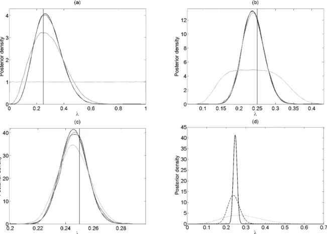
The estimated posterior distributions obtained according to Algorithm 2 using 1,000,000 simula-tions, together with the analytical posterior as in (2.2), are shown in Figure 2.3 for the dataset sizesn= 20, 200 and 2,000 respectively. The mean, the median and the 95 % credible interval 2 of the posteriors are presented in Table 2.1, as well as the number of accepted simulations.

When bothand the dataset size are 20, allλ’s generated from the prior will be accepted, i.e. the resulting posterior equals the prior. This can be viewed as the extreme of the fundamental property in ABC; when goes to infinity, the posterior distribution will take the form of the prior. One can see that the choice of clearly affects the outcome of the algorithm, even though the median and mean of the posteriors in all cases but the one just mentioned are estimated very well (Table 2.1). As an example; when the dataset sizen= 20, only a zero tolerance will result in a fully satisfactory posterior (Figure 2.3a), even though the one obtained by= 2 might be usable too, depending on preferences. For comparison, the analytical posterior distributions for all three datasets are shown in Figure 2.3d. So, why would one want to use a non-zero tolerance? Because of the same reason as one is using a tolerance in the first place, to improve sampling efficiency. For example, when the dataset size n= 2,000, a zero tolerance and = 20 give similar posteriors (Figure 2.3c and Table 2.1), but the latter consists of 20,718 acceptedλ’s and the former of only 518.

2

(10)

Figure 2.3: Markov model example using ABC. The analytical posterior (black) together with the estimated posteriors of λfor= 0 (dark-grey), = 2 (medium-grey) and = 20 (light-grey) for dataset sizes n= 20 (a), 200 (b) and 2000 (c). These are obtained by Algorithm 2 and 1,000,000 simulations each and shown are the estimated kernel densities of the posteriors using Matlab’s ksdensity. In (d), the analytical posteriors for dataset sizes n = 20 (dotted), 200 (dashed) and 2,000 (solid) are shown. The observed datasets are generated usingλ= 0.25, indicated by the vertical lines.

(11)

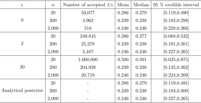
n Number of accepted λ’s Mean Median 95 % credible interval 0 20 50,077 0.286 0.279 [0.119,0.490] 200 4,962 0.239 0.238 [0.182,0.298] 2,000 518 0.246 0.246 [0.228,0.266] 2 20 249,845 0.286 0.277 [0.088,0.532] 200 25,278 0.239 0.238 [0.181,0.301] 2,000 2,487 0.246 0.246 [0.227,0.265] 20 20 1,000,000 0.500 0.501 [0.025,0.975] 200 204,928 0.239 0.238 [0.125,0.362] 2,000 20,718 0.246 0.246 [0.224,0.269] Analytical posterior 20 - 0.286 0.279 [0.119,0.491] 200 - 0.239 0.238 [0.183,0.300] 2,000 - 0.246 0.246 [0.227,0.265]

Table 2.1: Markov model example using ABC. The mean, median and 95 % credible interval of the posteriors ofλin Figure 2.2 when using ABC as well as of the exact posterior. For the ABC, the number of accepted λ’s is also reported, out of 1,000,000 simulations each. The datasets are generated usingλ= 0.25.

(12)

2.2.2 Example of hidden Markov model

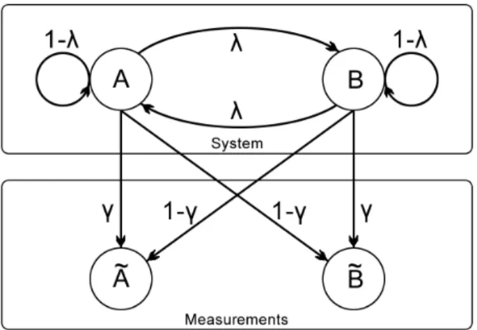
The second model to be studied is the hidden Markov model in Figure 2.4, a model where mea-surement error is accounted for. It uses a Markov model for an unseen (hidden) Markov chain, as in Figure 2.2, with transition probabilityλ. This chain is hidden since there is also a measurement procedure, where the probability of correct measurement isγ.

Figure 2.4: The hidden Markov model considered, whereλis the probability of switching from A to B and vice versa, whileγis the probability of making a correct measurement.

Data of this type is referred to as noisy data and is typically non-Markovian. As in the previous example, a dataset is generated from this model with given λand γ, namely 0.25 and 0.90. Once again, the posteriors are estimated using Algorithm 2 for dataset sizes n= 20, 200 and 2000 and tolerances = 0, 2 and 20. The starting character is again chosen from a discrete uniform density on A and B. This time the exact posterior will not be found analytically, instead the result will be compared to the one obtained by likelihood-free MCMC in chapter 3. Still, no knowledge ofλ is assumed, and thus a U(0,1) prior is used for this parameter. Since in the HMM a measurement process is considered, it is reasonable to assume that the measuring instrument is decent, and thus aBeta(α, β) prior is chosen forγ. Too see how the choice of the prior affects the obtained posterior, this will also be estimated using two different sets of (α, β) for all three datasets and tolerances.

Results

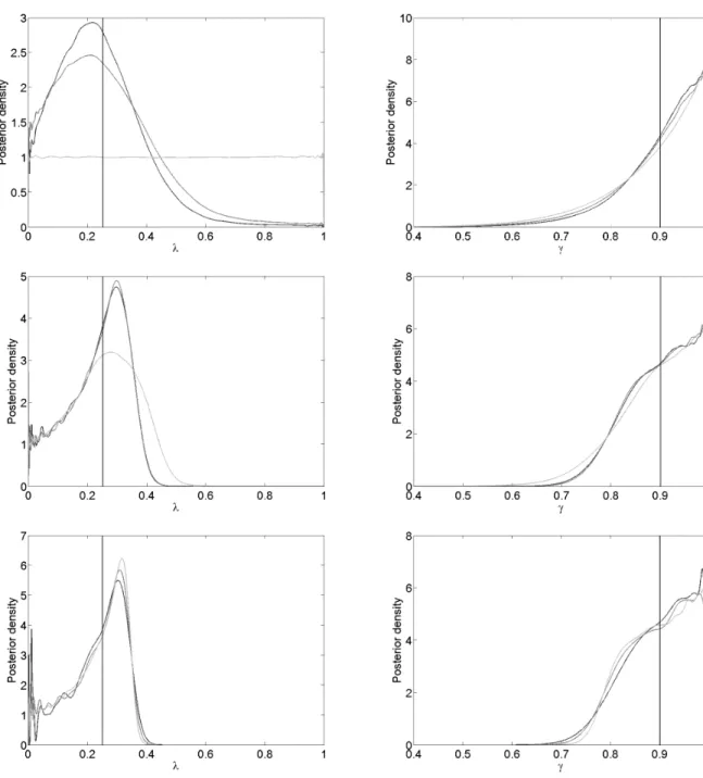
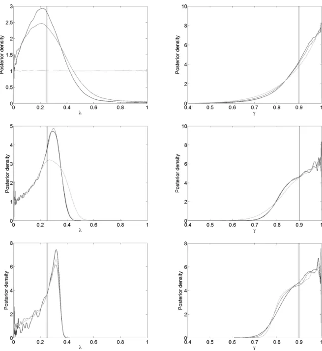
The estimated posterior distributions ofλand γ, using Algorithm 2 and 1,000,000 simulations and dataset sizes n = 20, 200 and 2,000 are shown in Figure 2.5, for tolerances = 0, 2 and 20 and hyperparameters for γ as (α, β) = (8,1). These hyperparameters yield a prior distribution with a high probability mass of exact measurement. The mean, the median and the 95 % credible interval of the posteriors are presented in Table 2.2, together with the number of accepted simulations. Now, assume that there are reasons to believe that the measuring instrument is good, but really not perfect (say the package states it measures correctly 95 % of the times), and put another prior with parameters (α, β) = (38,2), i.e. with mean 0.95. The estimated posterior distributions using the latter prior, and their corresponding data, are shown in Figure 2.6 and Table 2.3.

Again, one can see that the effect to the estimated posterior of the tolerance decreases as the dataset size increases for both choices of prior, as would intuitively be the case. When both the dataset size

(13)

Figure 2.5: Hidden Markov model example using ABC. The estimated posteriors ofλandγfor= 0 (dark-grey), = 2 (medium-grey) and = 20 (light-grey) for dataset sizes n= 20 (top), 200 (middle) and 2000 (bottom). These are obtained by Algorithm 2 and 1,000,000 simulations each and shown are the estimated kernel densities of the posteriors using Matlab’sksdensity. Here the hyperparameters forγare (α, β) = (8,1) and the true parameter values are (λ, γ) = (0.25,0.90), indicated by the vertical lines.

and the tolerance are 20, the samples are distributed according to the prior distributions. In this case, all the posteriors ofγ are very similar to the prior in both cases. A fundamental property of Bayesian analysis is that the impact of the prior decreases as more data is collected [11]. This can be noted for both sets of hyperparameters in Figure 2.5 and Figure 2.6. For the second choice of

(14)

hyperparameters, (α, β) = (38,2), this effect is not as clear as when using (α, β) = (8,1), indicating either astronger or a more posterior-resemblant prior. Stronger in the sense of a more concentrated probability mass.

Parameter n Number of acceptedλ’s Mean Median 95 % credible interval

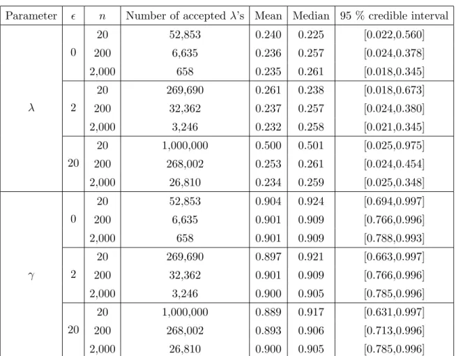
λ 0 20 52,853 0.240 0.225 [0.022,0.560] 200 6,635 0.236 0.257 [0.024,0.378] 2,000 658 0.235 0.261 [0.018,0.345] 2 20 269,690 0.261 0.238 [0.018,0.673] 200 32,362 0.237 0.257 [0.024,0.380] 2,000 3,246 0.232 0.258 [0.021,0.345] 20 20 1,000,000 0.500 0.501 [0.025,0.975] 200 268,002 0.253 0.261 [0.024,0.454] 2,000 26,810 0.234 0.259 [0.025,0.348] γ 0 20 52,853 0.904 0.924 [0.694,0.997] 200 6,635 0.901 0.909 [0.766,0.996] 2,000 658 0.901 0.909 [0.788,0.993] 2 20 269,690 0.897 0.921 [0.663,0.997] 200 32,362 0.901 0.909 [0.766,0.996] 2,000 3,246 0.900 0.905 [0.785,0.996] 20 20 1,000,000 0.889 0.917 [0.631,0.997] 200 268,002 0.893 0.906 [0.713,0.996] 2,000 26,810 0.900 0.905 [0.785,0.996]

Table 2.2: Hidden Markov model example using ABC. The mean, median and 95 % credible interval of the posteriors of λand γ in Figure 2.4 when using Algorithm 2 with hyperparameters for γ as (α, β) = (8,1). The number of acceptedλ’s andγ’s is also reported, out of 1,000,000 simulations each. The true parameter values are (λ, γ) = (0.25,0.90).

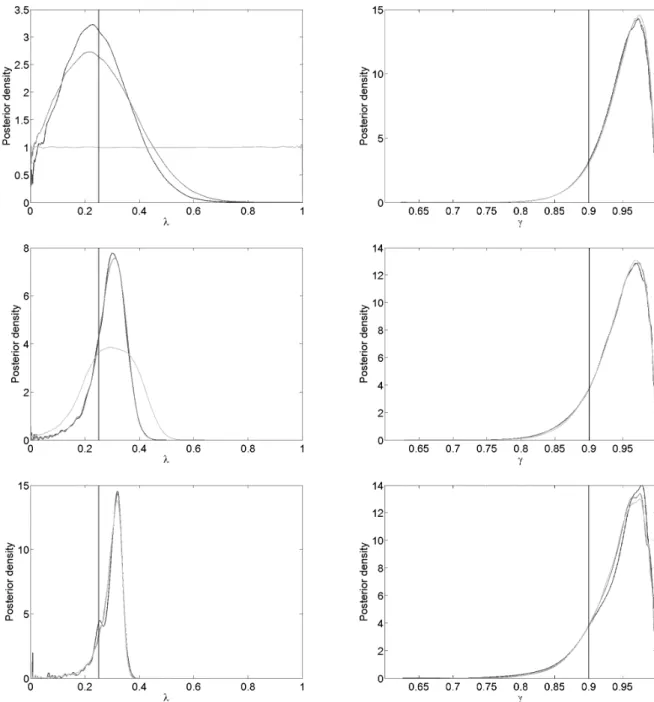
When comparing the posteriors obtained by using the two priors onγ, the modes are very similar, but the second (Beta(38,2)) have induced less mass in the lower region ofλ. This has led to a clear overestimation of both λ and γ, while the first prior (Beta(8,1)) seems to give better estimates (cf. Table 2.2 and Table 2.3). Due to this sensitivity to the choice of prior, it is important to do a problem and model specific sensitivity analysis on the posterior with respect to the prior. It is evident that the value of the tolerance might have great effect on the resulting posterior, and the same type of analysis needs to be done also for the tolerance. Since zero tolerance gives the most accurate posterior, given the summary statistics, model and priors, e.g. the quadratic loss in comparison to this posterior as a function of the tolerance can be studied.

(15)

Figure 2.6: Hidden Markov model example using ABC. The estimated posteriors ofλandγfor= 0 (dark-grey), = 2 (medium-grey) and = 20 (light-grey) for dataset sizes n= 20 (top), 200 (middle) and 2000 (bottom). These are obtained by Algorithm 2 and 1,000,000 simulations each and shown are the estimated kernel densities of the posteriors using Matlab’s ksdensity. Here hyperparameters forγ are (α, β) = (38,2) and the true parameter values are (λ, γ) = (0.25,0.90), indicated by the vertical lines.

(16)

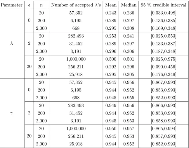
Parameter n Number of acceptedλ’s Mean Median 95 % credible interval λ 0 20 57,352 0.243 0.236 [0.033,0.498] 200 6,195 0.289 0.297 [0.136,0.385] 2,000 668 0.295 0.308 [0.169,0.348] 2 20 282,493 0.253 0.241 [0.025,0.553] 200 31,452 0.289 0.297 [0.133,0.387] 2,000 3,191 0.296 0.306 [0.187,0.348] 20 20 1,000,000 0.500 0.501 [0.025,0.975] 200 256,211 0.292 0.296 [0.090,0.456] 2,000 25,918 0.295 0.305 [0.176,0.349] γ 0 20 57,352 0.945 0.956 [0.867,0.993] 200 6,195 0.944 0.952 [0.853,0.993] 2,000 668 0.945 0.955 [0.852,0.993] 2 20 282,493 0.949 0.956 [0.866,0.993] 200 31,452 0.944 0.952 [0.853,0.993] 2,000 3,191 0.945 0.953 [0.858,0.993] 20 20 1,000,000 0.950 0.957 [0.865,0.994] 200 256,211 0.945 0.953 [0.857,0.993] 2,000 25,918 0.944 0.952 [0.852,0.993]

Table 2.3: Hidden Markov model example using ABC. The mean, median and 95 % credible interval of the posteriors ofλandγ in Figure 2.4 when using Algorithm 2 with hyperparameters forγ as (α, β) = (38,2). The number of acceptedλ’s andγ’s is also reported, out of 1,000,000 simulations each. The true parameter values are (λ, γ) = (0.25,0.90).

(17)

Chapter 3

Likelihood-free MCMC

3.1 Using ABC

Likelihood-free inference, including the ABC previously considered, can be seen in the way that it replaces the posterior in eq. (1.2) (called target posterior) by the augmented posterior

π(θ, x|y)∝π(y|x, θ)π(x|θ)π(θ), (3.1) where x is considered an auxiliary parameter, simulated from π(x|θ) as before. The function π(y|x, θ) is called weight function, since it induces high values for the posterior whenx and y are similar. For the case when x = y, π(y|x, θ) is assumed to have a maximum with respect to θ. Furthermore, the marginal posterior π(θ|y) is

π(θ|y)∝π(θ) Z

Y

π(y|x, θ)π(x|θ)dx. (3.2) Practically, one often targets the posterior π(θ, x|y) whereafter the x’s are ignored.

The augmented posterior π(θ, x|y) will be targeted as the stationary distribution of a generated Markov chain of{θt, xt}t≥0, using a Metropolis-Hastings (MH) MCMC algorithm. This is

theoret-ically done by using Algorithm 3, wherer((θ0, x0)|(θ, x)) is the proposal distribution. Algorithm 3: The Metropolis-Hastings algorithm withπ(θ, x|y) as stationary distribution.

1. Initialise (θ0, x0). Sett= 0.

At step t:

2. Generate (θ0, x0)∼r((θ, x)|(θt, xt)) from a proposal distribution.

3. Set (θt+1, xt+1) =      (θ0, x0), with probability 1∧ π(θ0,x0|y)r((θt,xt)|(θ0,x0)) π(θt,xt|y)r((θ0,x0)|(θt,xt)) (θt, xt), otherwise 4. Increment t=t+ 1 and go to 2.

(18)

The acceptance rate in this MH algorithm can be rewritten into a likelihood-free expression if a trick proposed by [8] is used. That is, by only consider proposal distributions of the form

r (θ0, x0)|(θ, x)

=r(θ0|θ)π(x0|θ0).

By using a proposal distribution of this form and by using the proportional expression for the augmented posterior in eq. (3.1), the acceptance rate in Algorithm 3 can be reformulated according to π(θ0_,x0_|_y₎_r₍₍_θ,x₎_|₍_θ0_,x0₎₎ π(θ,x|y)r((θ0_,x0₎_|₍_θ,x₎₎ = π(y|x0_,θ0₎_π₍_x0_|_θ0₎_π₍_θ0₎_r₍_θ_|_θ0₎_π₍_x_|_θ₎ π(y|x,θ)π(x|θ)π(θ)r(θ0_|_θ₎_π₍_x0_|_θ0₎ = π_π(y₍|_yx_|_x,θ0,θ0₎)_ππ₍(_θθ₎0_r)₍r_θ(0θ_||_θθ₎0).

The likelihood-free Metropolis-Hastings algorithm invoking this acceptance rate and type of pro-posal distribution is shown in Algorithm 4, where π(y|x, θ) is the weight function based on

some tolerance (named likelihood-free MCMC algorithm (LF-MCMC) in [8]). This algorithm will not have the exact augmented posterior π(θ, x|y) as stationary distribution, but instead π(θ, x|y) ∝π(y|x, θ)π(x|θ)π(θ) where suggests it is based on ABC and a tolerance . However,

just as in section 2.1, we let this be an approximation of the true augmented posterior π(θ, x|y). Once again, the target posterior will not be recovered exactly unless the set of summary statistics is sufficient and the toleranceis zero [8].

Algorithm 4: The likelihood-free MCMC algorithm, originating from [8]. 1. Initialise (θ0, x0) and . Sett= 0.

At step t:

2. Generateθ0∼r(θ|θt) from a proposal distribution.

The distribution π(θ, x|y) beeing the stationary distribution of the Markov chain generated by

Algorithm 4 means that the produced sequence of {θt, xt}t≥0 will be of the desired distribution

asymptotically, i.e. whent goes to infinity. Therefore, one defines aburn-in {θt, xt}t=0,...,B

where-after the distribution of the generated sequence is considered to be sufficiently close to the stationary distribution. However, choosing B is not elementary and will be done by studying the trajectory of the sampled sequence, i.e. by choosing B to the point whereafter the sampled sequence seems to have reached its stationary distribution. In Algorithm 4 and in algorithms originating from the same, x0 needs to be consistent with y. That is, ify is assumed to be noisy so is x0 and if y is not

(19)

nor isx0. In words of the previous examples: x0 is generated from the model in Figure 2.2 or Figure 2.4 ify is considered noise-free or noisy, respectively.

Typically, the samples should be uncorrelated for Monte Carlo integration to hold. For MCMC integration though, the ergodic theorem is often called for, implying that the integration is still valid if the number of samples goes to infinity, even though the samples in MCMC are correlated. Clearly, there is a trade-off between these two effects. If the number of samples is large enough, the effect of the samples beeing correlated might be averaged out in the inference [12]. Since the number of samples is finite, fewer and less correlated samples might give better inference. One way of constructing less correlated samples is bythinning, i.e. keeping everynth sample and and choose nsuch that the autocorrelation function reaches a sufficiently low value desirably fast. The latter will be done, aiming for the autocorrelation to be negligible at lag 30–50.

3.1.1 The HMM example

Once again, the hidden Markov model in Figure 2.4 will be considered, but this time using the likelihood-free MCMC algorithm described in Algorithm 4. The same datasets of lengths 20, 200 and 2,000 as well as priors forλandγ as in section 3.1 are used, while the proposal distributions of λand γ are chosen to be independent truncated Gaussian distributions, to the intervalI= [a, b] = [0,1], according to r_θi(z|θi_t) =              0, ifz≤a f_θi(z|θi t) F_θi(b|θi t)−Fθi(a|θ i t) , ifa < z < b 0, ifz≥b ,

wherei= 1,2, (θ1, θ2) = (λ, γ), θi∈ I,f_θi(z|θi_t) is the pdf of the Gaussian distribution with mean

θi_tandFθi(z|θi_t) is its cdf, with inverseF−1

θi (z|θti). Pseudorandom numbers distributed according to

this distribution are drawn using the inverse transform sampling. That is, by using the fact that Z =R−_θi1(U|θti)∼rθi(z|θi_t) ifU ∼ U(0,1), where R−1

θi is the inverse cdf ofrθi according to

Since the proposal distributions ofλand γ are independent, it holds that rθ(z|θt) =rλ(z|λt)·rγ(z|γt)

and because of the independence of the priors, π(θ) = π(λ)π(γ). Therefore, Algorithm 4 can be reformulated to Algorithm 5 in the HMM example. Proposals generated in this way are said to

(20)

follow a Metropolis-Hastings random walk.

Algorithm 5: The likelihood-free MCMC algorithm adapted for the HMM example. 1. Initialise (θ0, x0) and . Sett= 0.

At step t:

2. Generateλ0 ∼rλ(z|λt) from a proposal distribution.

3. Generateγ0 ∼rγ(z|γt) from a proposal distribution.

4. Setθ0= (λ0, γ0).

As a weight function, theuniform kernel density as described in [8] is chosen, i.e.

π(y|x, θ)∝      1, ifρ(T(x), T(y))≤ 0, otherwise , (3.3)

where the summary statistic and the distance measure are the same as previously. Remember that since the observed datasetyis noisy, so is the generated x0 in Algorithm 5. That is,x0 is generated from the HMM in Figure 2.4, given both the proposedλ0 andγ0.

3.1.2 Results

Now, only the Beta(8,1)-prior will be used for γ while the one for λ is still U(0,1), and the posterior will be estimated through Algorithm 5. The datasets are the same used in section 2.2.2. The standard deviations of the proposal densities are chosen according to Table 3.2 to make the mean acceptance rates and chain mixing reasonable. An initial 1,000,000 steps were carried out according to Algorithm 5 for each dataset size n = 20,200 and 2,000 and tolerance = 0, 2 and 20. The mean acceptance rates, chosen burn-ins and thinning rates are declared in Table 3.2. The resulting trajectories are in Figure 3.2 – 3.4 and the estimated marginal posteriors of λand γ in Figure 3.1. Note that the trajectories are shown for illustrative purposes and will not be included later in the report. The number of resulting draws, the mean and the median of the estimated posteriors and their 95 % credible intervals are shown in Table 3.1. Note that thinning rates and burn-ins are accounted for in all results.

(21)

Figure 3.1: Hidden Markov model example using MCMC ABC. The estimated posteriors of λ and γ for = 0 (dark-grey),= 2 (medium-grey) and= 20 (light-grey) for dataset sizesn= 20 (top), 200 (middle) and 2,000 (bottom). These are obtained by Algorithm 5 and consist of draws according to the trajectories in Figure 3.2 – 3.4. Shown are the estimated kernel densities of the posteriors using Matlab’sksdensity. Here hyperparameters forγ are (α, β) = (8,1) and the true parameter values are (λ, γ) = (0.25,0.90), indicated by the vertical lines.

(22)

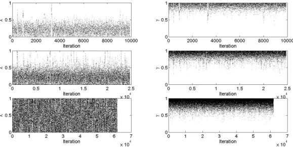
Figure 3.2: Hidden Markov model example using MCMC ABC. Trajectories of λ and γ for dataset size n= 20 and tolerances= 0 (top), 2 (middle) and 20 (bottom), obtained by Algorithm 5 according to Table 3.2. The hyperparameters forγare (α, β) = (8,1).

Figure 3.3: Hidden Markov model example using MCMC ABC. Trajectories of λ and γ for dataset size n= 200 and tolerances= 0 (top), 2 (middle) and 20 (bottom), obtained by Algorithm 5 according to Table 3.2. The hyperparameters forγare (α, β) = (8,1).

(23)

Figure 3.4: Hidden Markov model example using MCMC ABC. Trajectories of λ and γ for dataset size n= 2,000 and tolerances = 0 (top), 2 (middle) and 20 (bottom), obtained by Algorithm 5 according to Table 3.2. The hyperparameters forγare (α, β) = (8,1).

The posteriors estimated using MCMC are very similar to the ones usingraw ABC in section 2.2.2 (cf. Table 2.2 and 3.1). The most evident differences, still small, are in the estimated posteriors with zero tolerance at the dataset sizen= 2,000. This is probably explained by the fewer samples in raw ABC (658) than in MCMC (7,657); hence, the former posteriors might not have converged, with respect to Monte Carlo error. The more numerous samples in MCMC comes with the price of beeing correlated, in contrary to the ones in raw ABC, but since the two methods give very similar results otherwise this does not seem to be a valid cause for the observed difference.

3.2 Exact Bayesian inference

The exact Bayesian inference can be carried out by following the procedure in section 3.1 and Algorithm 5 with the exception that the weight function is not based on ABC, but instead its analytical expression. This will enable exact recovery of the target posterior. Once again, let y = (y1, y2, . . . , yn) be an observation of Y = (Y1, Y2, . . . , Yn), where all Yi’s are conditionally

independent given the hidden state X. Also, let x = (x1, x2, . . . , xn) be the generated dataset in

Algorithm 5, this time the hidden state of the HMM, i.e. generated according to Figure 2.2. By studying the HMM in Figure 2.4 one can conclude that

π(y|x, θ) = n Y i=1 π(yi|xi), (3.4) where π(yi|xi) =      γ, ifyi =xi 1−γ, ifyi 6=xi . (3.5)

(24)

Parameter n Number of drawn parameters Mean Median 95 % credible interval λ 0 20 9,900 0.239 0.224 [0.022,0.573] 200 30,625 0.237 0.258 [0.024,0.381] 2,000 7,657 0.249 0.274 [0.035,0.345] 2 20 24,750 0.267 0.242 [0.018,0.696] 200 122,500 0.237 0.257 [0.025,0.381] 2,000 15,000 0.233 0.260 [0.025,0.344] 20 20 61,875 0.499 0.497 [0.025,0.975] 200 122,500 0.253 0.260 [0.025,0.452] 2,000 122,500 0.235 0.261 [0.025,0.348] γ 0 20 9,900 0.904 0.925 [0.691,0.996] 200 30,625 0.902 0.910 [0.768,0.996] 2,000 7,657 0.910 0.917 [0.790,0.995] 2 20 24,750 0.894 0.920 [0.642,0.997] 200 122,500 0.901 0.910 [0.767,0.996] 2,000 15,000 0.900 0.906 [0.786,0.995] 20 20 61,875 0.889 0.917 [0.633,0.997] 200 122,500 0.893 0.907 [0.716,0.996] 2,000 122,500 0.901 0.907 [0.786,0.996]

Table 3.1: Hidden Markov model example using MCMC ABC. The mean, median and 95 % credible interval of the posteriors ofλandγin Figure 2.4 when using Algorithm 5 with hyperparameters forγas (α, β) = (8,1). The number of drawn λ’s andγ’s is also reported. An initial 1,000,000 step MCMC was made, the above shown result is after the burn-in and thinning is accounted for. Further execution information in Table 3.2. The true parameter values are (λ, γ) = (0.25,0.90).

That is, the weight function in the algorithm is calculated by first simulating a hidden datasetx0 from the Markov model, given the proposed λ0, whereafter π(y|x0, θ0) is evaluated by eq. (3.4), given the proposed γ0.

3.2.1 Results

By applying this theory to our HMM for the given dataset sizesn= 20, 200 and 2,000 one quickly realises one of the big advantages of ABC – the acceptance rate in the MCMC algorithm gets so low that the method is computationally in-feasible, already for n= 20. For comparison purposes, we apply both exact Bayesian inference and ABC to an observed dataset of sizen= 5. It is generated according to the HMM in Figure 2.4, given (λ, γ) = (0.25,0.90) and is y = (A, B, B, B, B). Of course, a dataset this short will typically not be best represented by the parameter set (λ, γ) = (0.25,0.90) and hence, it is not very likely that these parameter values are recovered from the inference. Anyhow, it should give insight in whether the ABC with the chosen summary statistic

(25)

n λ0 γ0 λstd γ std Tolerance () Burn-in Mean acceptance rate Thinning 20 0.5 0.9 0.05 0.05 0 10,000 9.7 % 100th 2 10,000 41.1 % 40th 20 10,000 79.9 % 16th 200 0.3 0.9 0.1 0.1 0 20,000 1.4 % 32nd 2 20,000 6.8 % 8th 20 20,000 43.5 % 8th 2000 0.25 0.9 0.1 0.1 0 20,000 0.2 % 128th 2 40,000 0.8 % 64th 20 20,000 6.5 % 8th

Table 3.2: Hidden Markov model example using MCMC ABC. Choices of initial parameter values, (λ₀, γ₀), and standard deviations (std) of the proposal densities for each dataset size n. For each tolerance and dataset sizen, the chosen burn-in and thinning rate are shown, together with the mean acceptance rate in Algorithm 5.

gives reasonable results, and in that case motivate our previous study on the HMM. For both the exact inference, i.e. when using a weight function in Algorithm 5 as in eq. (3.5), and for the ABC with weight function according to eq. (3.3), standard deviations for the proposal densities for both λand γ are chosen as 0.02. The initial parameter values are set to (λ0, γ0) = (0.5,0.9). As before,

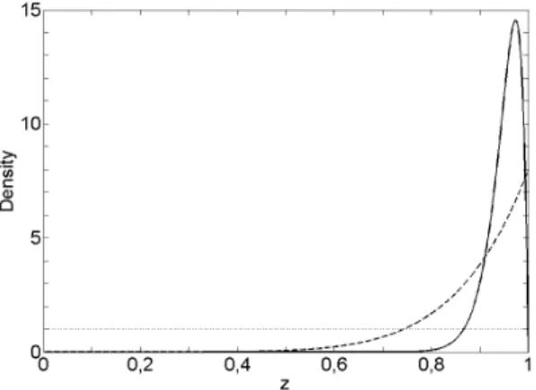
the prior for λ is U(0,1) while the one for γ is Beta(8,1). After a burn-in of 50,000 steps and a thinning rate of every 128th value for both runs the estimated posteriors, based on the 7,422 remaining samples, are seen in Figure 3.5. The posterior means and corresponding 95 % credible intervals for the exact Bayesian inference are, forλ, 0.372[0.022,0.903] and, forγ, 0.880[0.617,0.996], while they for the ABC are 0.360[0.028,0.854] and 0.889[0.635,0.997] respectively.

Figure 3.5: Hidden Markov model example using exact Bayesian inference. Estimated posteriors forλand γ using exact Bayesian inference (solid line) and MCMC ABC (dashed line). The observed dataset was generated using (λ, γ) = (0.25,0.90), indicated by the vertical lines.

(26)

Given the large sample size (7,422) it seems reasonable to assume that the observed difference between the estimated posteriors of the exact inference and the ABC is not due to Monte Carlo error but instead statistical bias. However, this is fairly small given the very simple summary statistic. Note that the estimated posteriors of γ are very similar to the prior, which is expected for such a short sequence. This small bias might not be a problem, depending on ones demand. However, as a try for decreasing the introduced bias we will in the next chapter consider a semi-automatic way of constructing summary statistics.

(27)

Chapter 4

Semi-automatic ABC

4.1 Theory

Choosing summary statistics is not always straightforward and, as mentioned before, these will most often be non-sufficient in practice; leading to an introduced bias. A procedure, called semi-automatic ABC (SA-ABC), is proposed by [13] and aims at high accuracy of specific estimates of θ instead of trying to minimise the error of the full posterior. This accuracy is defined in terms of the quadratic loss function of θ which, in the limit of → 0, is minimised if the summary statistics are the true posterior means, i.e. if T(y) = E(θ|y). The minimum loss in ABC occurs when ˆθ = E(θ|T(y)). That is, by using the quadratic loss function one tries to match the ABC posterior mean with the mean of the true posterior.

The true posterior means, to be used as summary statistics, are obviously unknown; otherwise the inference would be done. The idea is to model how the posterior means depend on the dataset, by Algorithm 6.

Algorithm 6: Semi-automatic ABC, as presented in [13].

1. Use a pilot run of ABC to determine a region, calledtraining region, of non-negligible posterior mass.

2. Simulate M sets of parameter values,θ1

i, . . . , θMi fori= 1, . . . , pwhere p= dim(θ) from the

priors truncated to the training region and simulate corresponding datasets y1_sim, . . . , y_simM . 3. Use the simulated sets of parameter values and simulated datasets to estimate the summary

statistics.

4. Run ABC with this choice of summary statistics.

The first step of the algorithm is not necessary in general, but important if the priors are uninfor-mative, and has the purpose of defining the training region from which the M parameter values are drawn in the second step. These are drawn from the priors, truncated to this training region, whereafter corresponding datasets are simulated from the model, given the parameter values. The motivation of this training region is that we want to base the the estimation ofE(θi|ysim) in

(28)

instead based on draws from other regions the risk is that the obtained summary statistics are not working satisfactorily. If the priors are informative, and based on some knowledge, the first step is however optional since then there is knowledge of where most of the posterior mass is located. In the third step of the algorithm, [13] suggests using linear regression with a vector-valued function f(·) of the dataset as predictors. This constitutes the ”semi” part of semi-automatic ABC, since f(·) needs to be chosen in the way thatf(ysim) is a vector of dataset transformations, which might

be non-linear. The linear regression will give one summary statistic for each parameter, using the drawn parameter valuesθ1_i, . . . , θ_iM from the second step as the responses andf(y_sim1 ), . . . , f(y_simM ) as explanatory variables. The model

θi=E(θi|ysim) +i =β0i +βif(ysim) +i, (4.1)

with mean-zero noise i, is fitted using least squares and hence ˆβi0 + ˆβif(ysim) is an estimate of

E(θi|ysim). These summary statistics are only estimates of the marginal posterior means, and as

such there is no mathematical result that guarantees that the scheme in Algorithm 6 produces a posterior distribution with minimised quadratic loss ofθ at the mean. Since one uses the distance between the summary statistics of the simulated and the observed dataset in ABC, the intercepts will cancel out and the summary statistic for theith parameter is chosen to beTi(ysim) = ˆβif(ysim)

[13].

Finally, in the fourth step, the ABC is run using these summary statistics. In [13] it is suggested to truncate the priors to the training region also for this step. However, here, the priors are used without truncation and the summary statistics are assumed to hold extrapolatively also outside the training region.

4.2 The HMM example

In the previous sections, the summary statistic has been chosen arbitrarily as the number of switches between the two characters A and B. This summary statistic will still be used in the first step of Algorithm 6, i.e. in the pilot run, to define the training region. Since the aim is to improve the result found in section 3.1.2, the tolerance used for the pilot run will be zero. That is, the pilot run is executed according to Algorithm 5 with pilot = 0 and the number of switches betweenA and B

as summary statistic. The training region used is the 98% credible interval and the prior for λis once again U(0,1) while the one for γ is Beta(8,1). This time, only the dataset of size n = 200 will be considered. For the linear regression in the third step of Algorithm 6, the function f(·) is chosen to capture reasonable characteristics of the dataset such that

f(ysim) = (Number of switches betweenA and B in ysim, Number of A’s inysim,

Max. number of subsequentA’s in ysim, Min. number of subsequentA’s inysim).

(4.2) For the semi-automatic ABC, i.e. the fourth step in Algorithm 6 and run according to Algorithm 5, the distance measure ρ(·,·) is once again the euclidean distance.

(29)

4.2.1 Results

The pilot run (first step of Algorithm 6), i.e. when using the tolerance = 0 and the number of switches as summary statistics in Algorithm 5 was executed for 1,000,000 steps using a burn-in of 20,000, a thinning rate of every 32nd value, initial values (λ0, γ0) = (0.30,0.90) and proposal

density standard deviations for both λ and γ as 0.1. This resulted in 30,625 drawn parameter values, a mean acceptance rate of the algorithm as 1.4 % and training regions [0.012,0.395] and [0.745,0.999] forλand γ respectively.

In the second step of Algorithm 6,M = 100,000 parameter values and corresponding datasets were simulated from the priors truncated to these training regions and the HMM in Figure 2.4. Applying the linear regression, eq. (4.1), in the algorithm’s third step with the functionf(·) chosen as in eq. (4.2), yielded regression coefficients as

ˆ

βλ = (0.00327, 0.00030, -0.00156, 0.00198)

ˆ

βγ = (-0.00226, 0.00029, -0.00141, 0.00097).

(4.3)

The fourth step of Algorithm 6 consists of Algorithm 5 with summary statistics as ˆβif(·) with

ˆ

βi according to eq. (4.3). With initial parameter values (λ0, γ0) = (0.30,0.90), proposal density

standard deviations 0.1 for both λ and γ and a tolerance = 0.001, an initial 5,000,000 steps of Algorithm 5 were run, resulting in a mean acceptance rate of 1.9 %. After a burn-in of 50,000 and a thinning rate of every 256th value, 19,336 draws remained giving the marginal posteriors estimates ofλand γ in Figure 4.1. Their means and 95 % credible intervals are 0.259[0.061,0.387] forλand 0.915[0.774,0.997] for γ while their medians are 0.276 and 0.926 respectively.

Figure 4.1: Hidden Markov model using SA-ABC. The estimated posteriors ofλandγ for the dataset size n = 200. These are obtained by Algorithm 6 with the final step according to Algorithm 5 with tolerance = 0.001. Shown are the estimated kernel densities of the posteriors using Matlab’sksdensity. The true parameter values are (λ, γ) = (0.25,0.90), indicated by the vertical lines.

The observed dataset, this time only the size n= 200 is considered, is once again identical to the one of the same size used in previous chapters. Therefore, the results found by semi-automatic ABC will be compared to what was found by Algorithm 5 for the same observed dataset when the number of switches betweenA and B was used as summary statistic (Figure 3.1 and Table 3.1 for

(30)

= 0; which is the same run used as the pilot). As previously stated, this semi-automatic ABC aims at matching the approximated posterior mean with the true posterior mean. The estimated posterior means were (ˆλSA,γˆSA) = (0.259,0.915) and (ˆλ,γˆ) = (0.237,0.902) in the semi-automatic

ABC and the pilot respectively. By the first look, one might be led to conclude that the semi-automatic ABC did a better job at estimating λ while the pilot did better for γ. Though, this conclusion is somewhat rushed. Indeed, the observed dataset is generated using (λ, γ) = (0.25,0.9), but since the dataset is relatively short (200) and the generation is stochastic, we can not be sure that this dataset is perfectly representative of this set of parameters. For this example, the effect of using semi-automatic ABC is probably not so large since the number of switches betweenA and B seems to be a relatively good summary statistic. To really see the effect, one could study the mean quadratic loss for a set of different observed datasets, all generated using (λ, γ) = (0.25,0.90) (see [13] where this is done). In this way, the above mentioned uncertainty in whether the observed dataset is representative of (λ, γ) would cancel out, as well as other variations. This would show if the semi-automatic ABC in general improves the mean of the estimated posterior in this example. The 95 % credible intervals ofλandγ decreased by 9 % and 2 % respectively, using semi-automatic ABC (cf. Table 3.1). The reason could be that the summary statistics of the semi-automatic ABC are closer to sufficient than the one used in the pilot. It could also be due to the obtained possibility to choose the tolerance arbitrarily low since the summary statistics have a continuous state space; in contrary to the discrete state space of the summary statistic in the pilot where a zero tolerance was the best possible. Logically for non-sufficient summary statistics, there should be a lowest under which no extra precision is gained, whereas the acceptance rate is reduced. Our choice of tolerance, = 0.001, might be below this limit since this has not been studied. An idea for this is to study the previously mentioned mean quadratic loss, for different choices of. This time, we settle at observing that the semi-automatic ABC seems to work satisfactorily.

(31)

Chapter 5

ABC in a Stochastic Lotka-Volterra

model

5.1 Varying bandwidth

Now, we aim at improving the likelihood-free MCMC algorithm in Algorithm 4, as is done in [14]. As before, an approximation to the weight function π(y|x, θ) is needed. A commonly used approximation is π(y|x, θ) = 1 K ρ(T(x), T(y)) , (5.1)

whereK(·) is a standard smoothing kernel centred atT(x) =T(y) and >0 now takes the role as bandwidth. As in [8], we defineK(·) as the uniform kernel density, why eq. (5.1) equals eq. (3.3). As previously mentioned, there is a trade-off in choosing in the sense that a low gives high statistical accuracy and low acceptance rate while a highinduces a higher probability of acceptance and a poorer statistical accuracy. The first idea of improvement tries to exploit both sides of this trade-off by considering the bandwidthan unknown parameter with its own Markov chain [15]. Let π() be the prior distribution of, and let the euclidean distance be the distance measure of choice and denote itρ(T(x), T(y)) =|T(x)−T(y)|. As in [14] we will always use the Metropolis random walk with Gaussian increments. Since the Gaussian increments are symmetric, the acceptance rate can be simplified according to

K(|T(x0)−T(y)|/0)π(θ0)π(0)r(θt, t|θ0, 0)

K(|T(xt)−T(y)|/t)π(θt)π(t)r(θ0, 0|θt, t)

= K(|T(x

0₎₋_T₍_y₎_|_/0₎_π₍_θ0₎_π₍0₎

K(|T(xt)−T(y)|/t)π(θt)π(t)

Using this, Algorithm 4 can be extended to Algorithm 7. Once again, the simulated dataset x0 needs to be consistent with the observed dataset y, in the sense that they are both subject to measurement error or both are not. After the simulations, the Markov chain {θt}t≥0 is filtered by

discarding all {θt|t≤∗}, where the threshold ∗ is chosen case specifically. This threshold is set

by studying how the posterior distribution mean and 95 % credible interval of {θt}t≥0 vary with

respect to by plotting these of {θt|t≤∗}against the all possible ∗ [15]. To keep the bias low,

a small ∗ is desirable. Though, this might result in few remaining parameter values and a large Monte Carlo error, why a larger∗ might be favourable. Therefore, we select the smallest∗ giving a reasonably accurate posterior and a satisfactory long sequence of θ. For example, if one wants

(32)

to approximate the mean of the posterior, [14] suggests to choose ∗ such that the posterior mean in the bandwidth plot is approximately constant but still high enough to result in a long enough sequence ofθ.

For a very interesting way of accelerating the computation, see [14] where a so calledEarly-Rejection can allow for occasional rejection of a proposal without the need of simulating x(the paper states an acceleration of 40-50 % in its applications).

Algorithm 7: The likelihood-free MCMC algorithm, with a Markov chain also for the bandwidth. 1. Initialise (θ0, x0, 0). Sett= 0.

At step t:

2. Generate (θ0, 0)∼r(θ, |θt, t) from a proposal distribution.

3. Generatex0 ∼π(x|θ0) from the model givenθ0 and save T(x0). 4. Set (θt+1, t+1, T(xt+1)) =      (θ0, 0, T(x0)), with probability 1∧_KK₍(_||_TT₍(_xx0)−T(y)|/0)π(θ0)π(0) t)−T(y)|/t)π(θt)π(t) (θt, t, T(xt)), otherwise 5. Increment t=t+ 1 and go to 2.

5.2 Stochastic Lotka-Volterra real data study

As a real life example we will study the data of the yearly number of trapped Lynx and Snowshoe Hares in North Canada in [16] during the years 1900-1920, see Figure 5.1. In the mean, this is likely to give a good view of the true relative populations.

(33)

A famous model that incorporates this type of behaviour, the interaction between a predator and a prey, is the Lotka-Volterra predator-prey model in eq. (5.2), where x1 is the number of prey

(Snowshoe Hares), x2 the number of predators (Lynx), k∗1 the prey growth rate, k3∗ the predator

death rate andk2 the encounter rate of predator and prey [17].

dx1 = (k∗1x1−k2x1x2)dt

dx2 = (−k∗3x2+k2x1x2)dt

(5.2)

In this ordinary differential equation (ODE) all parameters k₁∗,k2 and k3∗ are considered constant.

However, it does seem more reasonable to assume that the prey growth rate k₁∗ and the predator death ratek₃∗ depend on numerous states, e.g. precipitation, temperature and hunting. These are assumed to vary stochastically such thatk₁∗ is substituted byk1+σ1ξ1,t andk∗3 =k3+σ2ξ2,t where

{ξ1,t}t≥0and{ξ2,t}t≥0are Gaussian white noise processes andk1,k3,σ1andσ2are parameters. The

parametersσ1 andσ2 represent the randomness ”intensities” of{ξ1,t}t≥0 and{ξ2,t}t≥0 respectively

[18]. Following this, the ODE in eq. (5.2) can be written as the stochastic differential equation in eq. (5.3). Capital X1 and X2 suggests that the model is stochastic while dW1 and dW2 are

independent increments of standard Brownian motions.

dX1 = (k1X1−k2X1X2)dt+σ1X1dW1

dX2 = (−k3X2+k2X1X2)dt+σ2X2dW2

(5.3)

As stated before, the data of the trapped animals should ”in the mean” reflect the true relative populations. Therefore, it is reasonable to assume some sort of an error model. Since not all Lynx and Hares of North Canada were trapped (or rather tracked in that case) there is an error between the true relative population and the observed. Other possible errors are ”miswriting” or failing of reporting the trapped animals. In any of these cases, it seems sensible to assume that the variability of the error increases with the population sizes. Therefore, we suggest an error model as in eq. (5.4), where Y is the trapped quantity andX its ”true” correspondence1.

Y1 =X1+ε1, ε1 ∼ N(0,(σεX1)2)

Y2 =X2+ε2, ε2 ∼ N(0,(σεX2)2)

(5.4)

The model in eq. (5.3), given the error model in eq. (5.4), is assumed to describe the data in Figure 5.1 and the parameters k1, k2, k3, σ1, σ2 and σε will be inferred using the semi-automatic ABC

scheme described in chapter 4, i.e. by Algorithm 6.

In [17] the same data is studied under the ODE model in eq. (5.2), except for that they separate the parameterk2into two parameters. However, their result and MLE of the parametersk1,k2andk3in

the ODE will be used to put informative priors on the same in the SDE. They found ˆk₁ODE = 0.556, ˆ

kODE₂ = 0.0275 (mean of the two new parameters) and ˆkODE₃ = 0.828. Since we have no knowledge of reasonable values of σ1 and σ2, eq. (5.3) was simulated using the MLE ofk1,k2 and k3 and the

SDE Toolbox [19] with the aim to find a reasonable interval forσ1 andσ2. Note that in the coming

analysis, the natural logarithm of the parameters will be studied, to enforce the parameter values

1

(34)

to stay positive. We found that reasonable priors for logσ1 and logσ2 are logσ1,logσ2 ∼ N(−2,1)

and by an educated guess, we put log(σε) ∼ N(−5.5,0.82). Priors for the other parameters are

chosen to be centred around the MLEs according to log(k1) ∼ N(log(ˆk1ODE),0.052), log(k2) ∼

N(log(ˆk₂ODE),0.22) and log(k3)∼ N(log(ˆk3ODE),0.052). We consider these priors informative and

as such, a pilot run and corresponding truncation in Algorithm 6 is not needed.

In the second step of Algorithm 6M = 840, since [14] suggests 10-20 timesd×nsimulated sets of parameters wheredis the dimension of the SDE (2), andy_sim1 , . . . , y_simM are full realisations of the SDE and consistent with the observed dataset, i.e. with added measurement error. Note that no truncation will be carried out since the priors are now considered informative. Using the function f(·) as the time ordered dataset, the summary statistics are determined in the third step according to the linear regression in eq. (4.1) using regression method Lasso.

The fourth step consists of Algorithm 7 where x0 is a full realisation of the SDE with added measurement error, the parameters of the SDE are considered mutually independent and the prior for the bandwidth is exponential with mean 0.05, i.e. ∼Exp(0.05). As starting values for the states we choose the initial observations X1,0 = 30 and X2,0 = 4 while the initial bandwidth is

set to 0 = 0.1. The SDE parameters’ initial values are the prior means. The inference is run

for 1,200,000 steps using the package abc-sde with numerical integration stepsize 0.02, a thinning of every 400th value, initial stepsizes for the Metropolis random walk as 0.01 for all parameters and a maximum value of the random walk for the bandwidthas max = 0.1. This package takes

advantage of the Early-Rejection mentioned previously, see [14] and [20]. After a burn-in of 120,000 steps, the bandwidth plots as described in section 5.1 with the solid line as the posterior mean and the 95 % credible interval illustrated by the dashed lines are seen in Figure 5.2. Following the theory in section 5.1 we choose∗= 0.07 in order to keep the posterior mean in the bandwidth plot approximately constant for all smaller bandwidths while still allowing for a long enough sequence. Note that there is a somewhat erratic behaviour for small bandwidths in Figure 5.2. This is what we want to cancel out by choosing a large enough to let the posterior be smooth, i.e. the erratic behaviour seen is a sign of the Monte Carlo error while the increased credible interval and added bias (hard to identify) for increasing bandwidth is the loss of statistical accuracy. This choice of ∗ leaves 902 samples of the marginal posterior of all parameters, whose priors and estimated marginal posteriors are seen in Figure 5.3. Using Bayes’ estimator, i.e. the mean of the posterior as an estimate for the parameters, estimates of the parameters in the SDE and corresponding 95 % credible intervals are ˆk1 = 0.550[0.511,0.597], ˆk2 = 0.0259[0.0238,0.0281], ˆk3 = 0.846[0.777,0.926],

ˆ

σ1 = 0.099[0.026,0.264], ˆσ2 = 0.080[0.023,0.323] and ˆσε = 0.0033[0.0009,0.0152]. The empirical

mean, 50 % and 95 % confidence intervals of 10,000 realisations of the SDE in eq. (5.3) in comparison to the observed dataset, using these estimates, are shown in Figure 5.4. A single, well-performing, realisation is visualised in Figure 5.5.

Given the model, the realisations in Figure 5.4 seem reasonable since the mean roughly follows the observed dataset. The confidence intervals of the ”peaks” clearly increase, which is intuitive since a small change in the prey growth rate (k1) or predator death rate (k3), especially at low numbers,

might give extremely different outcomes. To the writer this is known from the interaction between rodents and birds or Arctic Foxes in Scandinavia. Therefore, the results seem reasonable under the Lotka-Volterra model.

By looking at the marginal posteriors in Figure 5.3 one can see that they, for log(k1) and log(k3),

are similar to the priors. This is not surprising since the realisation of the SDE marginally changes with respect to these two parameters in the interval. However, these have physical meanings and

(35)

reasonable values. These priors have still been somewhat updated by the model and the data to the posteriors, why we consider the run computationally successful. The marginal posterior of σε

is also close to the prior. The reason could be that the observed dataset under the error model in eq. (5.4) is not well represented by the SDE model in eq. (5.3). Of course, a bad model is a possible cause of any unclear results. Another possibility is summary statistics which are far from sufficient. Therefore, it would have been interesting to compare the result to what is found by an exact inference, e.g. the one suggested by [2].

It is also unknown to what extent the discretisation of the SDE affects the inference in this case. The integration stepsize was chosen to the smallest value giving a reasonable execution time (around 6 hours on a well-performing laptop). It is possible that this discretisation is still too rough, resulting in a bias and hence might affect the inference heavily. A possible way of evaluating this impact is to run the inference for different stepsizes and compare the estimated marginal posteriors. The largest stepsize under which the marginal posteriors are negligibly altered would then be a small enough stepsize, kept as high as possible to maintain computational efficiency.

(36)

Figure 5.2: Lotka-Volterra study. Posterior means (solid lines) and 95 % credible intervals (dashed) for varying∗.

(37)

(38)

Figure 5.4: Lotka-Volterra study. Empirical mean (solid line), 50 % confidence interval (dotted line) and 95 % confidence interval (dashed line) for 10,000 realisations of the SDE in eq. (5.3) and observed dataset (rings), using the found parameter estimates.

(39)

(40)

Chapter 6

Closing comments

ABC offers a very interesting way of attacking complex models and their parameter estimations in cases when the likelihood function (model) is easily simulated from. It has proved to be easily implemented, even for complex models such as SDEs subjected to error models, while the execution parameters such as the standard deviation of the proposal density in the MH algorithm can be difficult to choose. For this, there is an interesting scheme called adaptive Metropolis algorithm proposed by [21]. It uses a zero-mean multivariate Gaussian distribution with covariance matrix Σ as proposal density, where Σ is continuously updated using the previous values of the simulation. There are several suggestions on how to treat the bandwidth in the MCMC algorithm. One proposal is the varying bandwidth introduced in section 5.1. Most challenging was to make sure the accep-tance rate did not turn too low, possibly affecting other parts of the algorithm negatively, while keeping the mean acceptance rate at a reasonable level. Of course, to prevent this, the bandwidth prior could have been truncated to exclude the lower regions. Another is by [8] which for eq. (3.3), if the parameter proposal is accepted, suggests to set a new tolerance t = max{,min{0, t−1}},

where0 =ρ(T(x0), T(y)) andis a lower limit. Otherwise,t=t−1. This way,tis asymptotically

the smallest value resulting in a non-zero weight function [8].

Throughout the thesis we have used thinning as a self-evident way of decreasing the correlation between the draws. There is an interesting article on this matter ([12]) which states that thinning is usually unsuitable if precision of parameter estimates is of highest concern.

These three suggestions would be interesting to evaluate or study if this work was to be extended. As a final suggestion, I would recommend [8] and [5] to you who want a great starting point for ABC.

Acknowledgements: I would like to thank Umberto Picchini for showing great interest in my learning and understanding.

(41)

Bibliography

[1] R. Turner (2008),Direct maximization of the likelihood of a hidden Markov model. Computa-tional Statistics and Data Analysis 52 (2008) pp. 4147-4160.

[2] D. J. Wilkinson (2011),Stochastic Modelling for Systems Biology. Chapman & Hall/CRC. [3] H. Sørensen (2004),’Parametric inference for diffusion processes observed at discrete points in

time: a survey. International Statistical Review, vol 72, no. 3, pp. 337-354.

[4] Tavar´e S, Balding D, Griffith R, Donnelly P (1997), Inferring coalescence times from DNA sequence data. Genetics 145(2):505-518.

[5] Marin, J. M., Pudlo, P., Robert, C. P., & Ryder, R. J. (2012), Approximate Bayesian compu-tational methods. Statistics and Computing, 22(6), 1167-1180.

[6] Pritchard J, Seielstad M, Perez-Lezaun A, Feldman M (1999), Population growth of human Y chromosomes: a study of Y chromosome microsatellites. Molecular Biology and Evolution 16:1791-1798.

[7] Marjoram P, Molitor J, Plagnol V, Tavar´e S (2003),Markov chain Monte Carlo without like-lihoods. Proceedings of the National Academy of Sciences 100(26):15,324-15,328.

[8] Scott A. Sisson and Yanan Fan (2010),Likelihood-free Markov chain Monte Carlo. In Handbook of Markov Chain Monte Carlo, Eds. S. P. Brooks, A. Gelman, G. Jones and X.-L. Meng. Chapman and Hall/CRC Press.

[9] Mikael Sunn˚aker, Alberto Giovanni Busetto, Elina Numminen, Jukka Corander, Matthieu Foll and Christophe Dessimoz (2013), Approximate Bayesian Computation. PLOS Computational Biology, Volume 9, Jan 2013.

[10] Christopher Nemeth, Hidden Markov Models with Applications to DNA Sequence Analysis. STOR-i, Lancaster University.

[11] Sk¨old, Martin (2006),Computer Intensive Statistical Methods. Lecture notes. Centre for Math-ematical Sciences, Lund University.

[12] Link, W. A. and Eaton, M. J. (2012), On thinning of chains in MCMC. Methods in Ecology and Evolution, 3. 112-115.

[13] Fearnhead P. and D. Prangle (2012), Constructing summary statistics for approximate Bayesian computation: Semi-automatic approximate Bayesian computation. J. Roy. Statist. Soc. B, 74 (3), 1-28.

(42)

[14] U. Picchini (2013), Inference for SDE models via approximate Bayesian computation. arXiv:1204.5459.

[15] P. Bortot, S.G. Coles and S.A. Sisson (2007), Inference for stereological extremes. Journal of the American Statistical Association, 477(102):84-92.

[16] E. P. Odum (1953),Fundamentals of Ecology. Philadelphia, W. B. Saunders. Data from http://www-rohan.sdsu.edu/∼_{jmahaffy/courses/f00/math122/labs/labj/q3v1.htm.}

[17] M. Gesmann (2012),Dynamical systems in R with simecol. K¨olner R User Group.

[18] B. Øksendal (2010), Stochastic Differential Equations: An Introduction with Applications. Springer.

[19] U. Picchini (2007),SDE Toolbox: Simulation and Estimation of Stochastic Differential Equa-tions with Matlab. http://sdetoolbox.sourceforge.net.

[20] U. Picchini (2013), abc-sde: a Matlab toolbox for approximate Bayesian computation (ABC) in stochastic differential equation models. https://sourceforge.net/projects/abc-sde/.

[21] H. Haario, E. Saksman, and J. Tamminen (2001),An adaptive Metropolis algorithm. Bernoulli, 7(2):223-242.