Note on Neural Network Sampling for
Bayesian Inference of Mixture Processes
Lennart F. Hoogerheide
∗& Herman K. van Dijk
†April 2007
Econometric Institute report EI 2007-15
Abstract
In this paper we show some further experiments with neural network sampling, a class of sampling methods that make use of neural network approximations to (posterior) densi-ties, introduced by Hoogerheide et al. (2007). We consider a method where a mixture of Student’s t densities, which can be interpreted as a neural network function, is used as a candidate density in importance sampling or the Metropolis-Hastings algorithm. It is ap-plied to an illustrative 2-regime mixture model for the US real GNP growth rate. We explain the non-elliptical shapes of the posterior distribution, and show that the proposed method outperforms Gibbs sampling with data augmentation and the griddy Gibbs sampler.
1
Introduction
Indirect simulation methods have made it possible to perform Bayesian analyses in many classes of models. The most well-known indirect simulation techniques are importance sampling [IS], introduced by Hammersley and Handscomb (1964) and introduced in econometrics and statistics by Kloek and Van Dijk (1978), and Markov chain Monte Carlo [MCMC] methods, such as the algorithms of Metropolis et al. (1953) and Hastings (1970) and the enormously popular Gibbs sampler, due to Geman and Geman (1984). However, there is, in practice, often doubt about the convergence behaviour of these methods. In some cases, the special features of the sampling method, the complex structure of the model, or the nature of the data may the reason that convergence would not even be reached for an infinite number of draws. In other cases, convergence would be reached in the limiting case of an infinite amount of draws; however, in practice, for any ‘reasonable’ amount of computing time the simulation results are unreliable. Examples of complex models are mixture models, in which a multimodal target density may occur. With the Gibbs sampler, reducibility of the chain may occur in this case: one of the modes may be missed completely. For the Metropolis-Hastings [MH] algorithm, if the candidate density is unimodal, with low probability of drawing candidate values in one of the modes, this mode may be missed completely, even when many draws are generated. In other cases, the acceptance probability may be very low, as many candidate values lying between the modes
have to be rejected. Using a unimodal normal or Student’stcandidate function, the method of
∗Center for Operations Research and Econometrics (CORE), Universit´e catholique de Louvain, Belgium †Econometric and Tinbergen Institutes, Erasmus University Rotterdam, The Netherlands
importance sampling ends up with many draws having only negligible weights. So, a common difficulty for the MH algorithm and IS is the choice of a candidate or importance density when (a priori) little is known about the shape of the target density.
For Bayesian inference in mixture models Fr¨uhwirth-Schnatter (2001) proposes the method
of permutation sampling. Geweke and Keane (2007) propose an MCMC method, using a Metropolis-Hastings step within the data augmentation approach, for smoothly mixing regres-sions, extending the conventional Bayesian mixture of normals model by permitting state prob-abilities to depend on observed covariates. MCMC methods with data augmentation are also considered by Geweke (2007). Bauwens et al. (2004) introduce the class of adaptive radial-based direction sampling [ARDS] methods to sample from target (posterior) distributions that are possibly highly non-ellliptical, for example multi-modal or extremely skew distributions. For this purpose, they make use of a transformation to radial coordinates. Hoogerheide et al. (2007) suggest a different approach. They introduce the class of neural network sampling methods, where a neural network approximation to the posterior density is used as a candidate density in IS or the MH algorithm. They propose three types of neural network functions that are easy
to sample from, when considered as density functions. One type is the adaptive mixture of t
densities [AdMit]. Among the neural network sampling methods, this approach appears to be the most efficient and reliable in several examples.
In this paper we consider the AdMit method of Hoogerheide and Van Dijk (2007), which is especially useful for models in which (some of) the parameters are restricted to a bounded domain, and where much posterior probability mass is located near boundaries. It is applied to an illustrative 2-regime mixture model for the US real GNP growth rate. We explain the non-elliptical shapes of the posterior distribution, and show that the proposed method outperforms several competing simulation methods including Gibbs sampling with data augmentation.
In Section 2 we present a summary of our method for constructing a proper candidate
distribution by iteratively adding Student’s t distributions to a mixture. For more details we
refer to Hoogerheide and Van Dijk (2007). In Section 3 we apply this method to the posterior distribution in an illustrative 2-regime mixture model for the US real GNP growth rate. Section 4 concludes with possibilities for future research.
2
Constructing approximations to posterior densities:
adaptive mixtures of t distributions
Suppose we have a data set y for which we assume a model with parameter vector θ ∈ Rk.
Suppose the aim is to investigate some of the characteristics of the posterior with density kernel
p(θ|y), for example the posterior mean and covariance matrix. Hoogerheide and Van Dijk (2007) suggest the following procedure:
1. Find a mixture of t densities q(θ) that approximates the posterior density with kernel
p(θ|y).
2. Obtain a sample of draws from the density q(θ).
3. Perform importance sampling or the (independence chain) Metropolis-Hastings algorithm using this sample in order to estimate characteristics of the posterior distribution ofθ.
There are two reasons for using mixtures of Student’s t densities. First, the class of mixtures
of Student’s tdensities possesses a certain ‘universal approximation property’. Zeevi and Meir
(1997) show that under certain conditions any density function may be approximated to
falls within their framework. This means that a wide variety of posterior distributions, for ex-ample multi-modal or highly skew distributions, can be approximated by mixtures of Student’s
tdensities. Second, a mixtures of Student’st densities is easily and quickly sampled from. The
Student’s t distribution is chosen instead of the normal, because it has fatter tails, so that the approach can more easily deal with fat-tailed posterior distributions.
We follow the three steps of Hoogerheide and Van Dijk (2007), where the first step consists
of the following iterative procedure to obtain an adaptive mixture of t densities [AdMit] that
approximates the posterior density p(θ|y). First, compute the mode µh and scale matrix Σh
of the first Student’s t density t(θ|µ1,Σ1, ν) in the mixture as the posterior mode, and minus
the inverse Hessian of logp(θ|y) evaluated at the posterior mode, respectively. We choose a
small degree of freedom parameter ν to allow for fat tails. Then draw a large set of points θi
(i= 1, . . . , N) from the ‘first stage candidate density’t(θ|µ1,Σ1, ν). After that, add components
to the mixture, iteratively, by performing the following steps:
Step 1: Check if the distribution of the importance sampling weights corresponding to the current candidate mixture distribution is ‘good enough’. If this is the case, then stop. Otherwise, go to step 2.
Step 2: Add another Student’st densityt(θ|µh,Σh, ν) to the mixture candidate density;
t(θ|µh,Σh, ν) covers a region of the parameter space where the current candidate density is much too small (as compared with the posterior density kernel p(θ|y)).
Step 3: Choose the probabilitiesP ph (h= 1, . . . , H) in the mixture candidate density H
h=1ph t(θ|µh,Σh, ν) by minimizing the (squared) coefficient of variation of the impor-tance sampling weights.
Step 4: Draw a sample ofN points θi (i= 1, . . . , N) from our new mixture of Student’s t distri-butions, PHh=1ph t(θ|µh,Σh, ν), and go to step 1.
For more details on the steps of this algorithm, we refer to Hoogerheide and Van Dijk (2007).
3
Example: 2-regime mixture model for real US GNP growth
In this section the AdMit approach that is discussed in Section 2, is applied to a highly non-elliptical, 4-dimensional posterior density in an illustrative model for the growth rate of the US real gross national product (GNP). The data that are used are the quarterly growth rates of the real US GNP in the period 1959-2001. The data are shown in Figure 1. In models for the GNP growth rate one often allows for separate regimes for periods of recession and expansion. In this section we consider a static 2-regime mixture model. In this model the (percentage) growth rate
yt, defined as 100 times the first difference of the logarithm of real GNP, has two different mean levels:
yt=
½
β1+εt with probabilityp
β2+εt with probability 1−p , t= 1,2, . . . , T, (1)
where εt ∼ N(0, σ2). For identification we assume that β1 < β2, so that β1 and β2 can be
interpreted as the mean growth rates during recessions and expansions, respectively. For the parameter vector θ = (β1, β2, σ, p)0 the prior kernel is specified as p(θ) ∝ 1/σ for β1 < β2,
0 ≤p≤1, and 0 elsewhere. Furthermore, β1 and β2 are restricted to the intervals [−3,2] and
[0,3], respectively.
It should be noted that this model is merely used as an example to illustrate the AdMit method in the case of a non-elliptical posterior distribution on a bounded domain, and to com-pare these with (Gibbs sampling with) data augmentation and the griddy Gibbs sampler. The
assumption that the ‘state’ (recession/expansion) is independent over (quarterly) observations is obviously unrealistic.
We use the AdMit approach (with N = 100000, M = 1000) to construct a mixture of
Student’st distributions that approximates the posterior distribution. Figure 2 shows the
non-elliptical shapes of a highest posterior density (HPD) credible set of (β1, β2, p) conditional
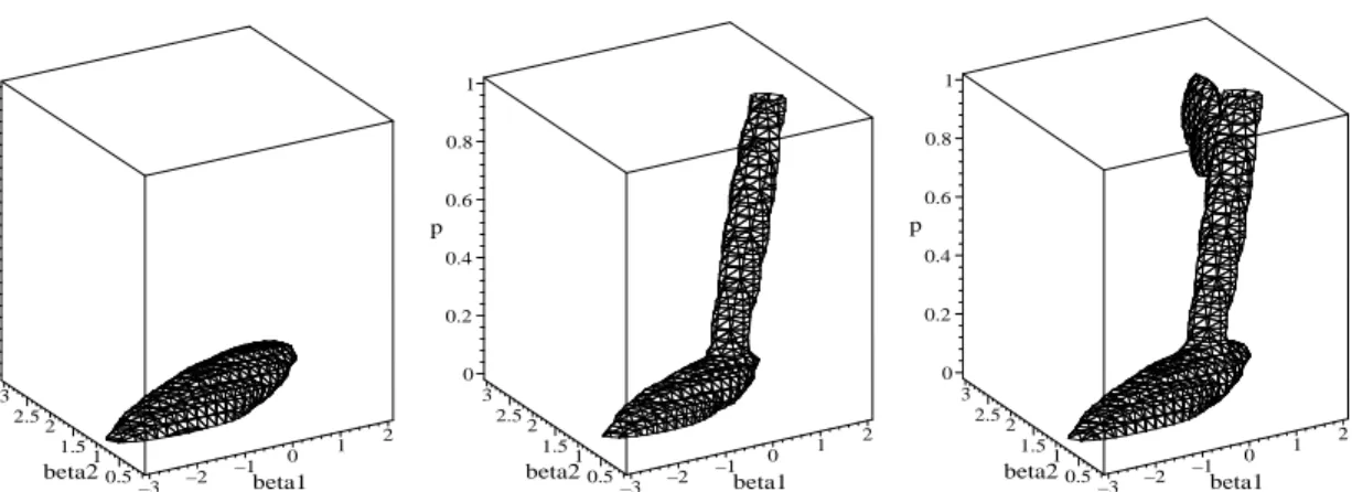
on σ = 0.79, the value of σ at the posterior mode (β1, β2, σ, p). Figure 3 illustrates the
iterative AdMit procedure by which a (mixture oft) candidate distribution is constructed: one
starts with a t distribution around the posterior mode, and iteratively adds t distributions
in areas where the previous candidate is too low, as compared with the posterior. It shows
that a mixture of 3 Student’s tdistribution can already provide a reasonable approximation to
the shape of the posterior distribution, reflecting that mixtures of t distributions can provide
reasonable approximations to a wide variety of posterior distributions. The AdMit method stops at a mixture of 5tdistributions, for which the ‘highest candidate density region’ is almost identical to the third panel of Figure 3.1 We use the mixture of 5t distributions as a candidate
distribution in IS and the MH algorithm; our aim is to obtain estimates of the posterior mean
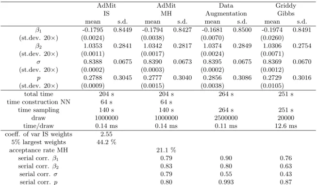
and standard deviation of β1, β2, σ and p. Table 1 shows the sampling results of AdMit-IS
and AdMit-MH. For AdMit-MH the posterior mean and standard deviation of each parameter are estimated as the average and standard deviation of the draws; for AdMit-IS the weighted analogues are reported.
Figure 4 shows histograms, scaled so that these can be interpreted as estimates of marginal
densities, of draws of β1,β2,σ,p obtained by the AdMit-MH method. Note the bimodality in
the marginal posteriors of β1 and p. The modes at β1 ≈ −1 and p ≈0.05 correspond with the
probability mass at the bottom of Figure 2, whereas the modes atβ1 ≈0.7 andp≈1 correspond
with the probability mass at the top of Figure 2. At the first region of the parameter spaceβ1
has the interpretation of the mean GNP growth rate during recessions which take place with low probabilityp. At the latter region of the parameter spaceβ1 has the interpretation of the mean
GNP growth rate during periods of low or medium growth which occur with large probabilityp,
whileβ2has the meaning of the mean GNP growth rate during ‘exceptional expansions’ (periods
of very high growth rates) occuring with low probability 1−p. Notice that forp= 0 (orp= 1)
the parameter β1 (or β2) is not identified. This local identification causes the highly
non-elliptical shapes in Figure 2: for low values of p a wide spectrum of β1 values is contained in
the HPD credible set, whereas for high values ofpthe HPD region contains wide intervals ofβ2
values.
In this model we can perform the method of Gibbs sampling with data augmentation of Tan-ner and Wong (1987). Data augmentation is used in order to sample from models with latent
variables Z, in which directly sampling the parameters θ seems very difficult, but sampling θ
given Z is straightforward. In this algorithm, the parameters θare drawn conditionally on the
latent variables Z, and the latent variables Z are drawn conditionally on θ. In our model we
define the latent 0/1 variables Zt (t = 1, . . . , T) as Zt = 1 (Zt = 0) if period t is a recession
(expansion) period. Conditionally on Z (and each other), β1 and β2 are normally distributed,
while σ2 and p have an inverted gamma and beta distribution, respectively. Conditionally on
the values of the parameters, the latent variablesZt (t= 1, . . . , T) have Bernoulli distributions. Another Gibbs sampling approach that can be applied in this example is the griddy Gibbs sampling approach of Ritter and Tanner (1992). In this approach, draws from the conditional distributions are obtained by applying the inversion method to a piecewise linear approxima-tion to the condiapproxima-tional cumulative distribuapproxima-tion funcapproxima-tion (CDF) that is computed using density
1Note that the approximation is certainly not perfect; however, a better approximation requires (possibly
much) more computing time in both the construction and sampling phase: there is a trade-off between the quality of the candidate mixture density and the speed of the construction and sampling.
1960 1965 1970 1975 1980 1985 1990 1995 2000 4000 6000 8000 real US GNP (level) 1960 1965 1970 1975 1980 1985 1990 1995 2000 −2 0 2 real US GNP (growth)
Figure 1: Real US GNP: quarterly growth rate in %. Source: Economagic.
–3 –2 –1 0 1 2 beta1 0.5 1 1.5 2 2.5 3 beta2 0 0.2 0.4 0.6 0.8 1 p
Figure 2: Highest posterior density (HPD) credible set for parameters (β1, β2, p) in a 2-regime mixture model for US real GNP growth rate (conditional on σ = 0.79, the value of σ at the posterior mode) –3 –2 –1 0 1 2 beta1 0.5 1 1.5 2 2.5 3 beta2 0 0.2 0.4 0.6 0.8 1 p –3 –2 –1 0 1 2 beta1 0.5 1 1.5 2 2.5 3 beta2 0 0.2 0.4 0.6 0.8 1 p –3 –2 –1 0 1 2 beta1 0.5 1 1.5 2 2.5 3 beta2 0 0.2 0.4 0.6 0.8 1 p
Figure 3: ‘Highest candidate density’ sets for a candidate Student’s t distribution around the posterior mode (left), a candidate mixture of 2 Student’stdistributions (middle), and a candidate mixture of 3 Student’s t distributions (right) for parameters (β1, β2, p) in a 2-regime mixture model for US real GNP growth rate (conditional on σ = 0.79, the value of σ at the posterior mode)
Table 1: Sampling results for the 2-regime mixture model for US real GNP growth
AdMit AdMit Data Griddy IS MH Augmentation Gibbs mean s.d. mean s.d. mean s.d. mean s.d.
β1 -0.1795 0.8449 -0.1794 0.8427 -0.1681 0.8500 -0.1974 0.8491 (st.dev. 20×) (0.0024) (0.0038) (0.0070) (0.0260) β2 1.0353 0.2841 1.0342 0.2817 1.0374 0.2849 1.0306 0.2754 (st.dev. 20×) (0.0011) (0.0017) (0.0024) (0.0071) σ 0.8388 0.0675 0.8390 0.0673 0.8395 0.0675 0.8369 0.0670 (st.dev. 20×) (0.0002) (0.0003) (0.0002) (0.0012) p 0.2788 0.3045 0.2777 0.3040 0.2856 0.3086 0.2729 0.3016 (st.dev. 20×) (0.0009) (0.0015) (0.0038) (0.0105) total time 204 s 204 s 264 s 251 s time construction NN 64 s 64 s time sampling 140 s 140 s 264 s 251 s draw 1000000 1000000 2500000 20000 time/draw 0.14 ms 0.14 ms 0.11 ms 12.6 ms coeff. of var IS weights 2.55
5% largest weights 44.2 % acceptance rate MH 21.1 % serial corr. β1 0.79 0.90 0.76 serial corr. β2 0.83 0.80 0.63 serial corr. σ 0.79 0.55 0.43 serial corr. p 0.80 0.993 0.87 0 0.2 0.4 0.6 0.8 1 –3 –2 –1 0 1 2 beta1 0 0.5 1 1.5 2 2.5 3 3.5 0 0.5 1 1.5 2 2.5 3 beta2 0 1 2 3 4 5 0 0.5 1 1.5 2 sigma 0 1 2 3 4 5 0 0.2 0.4 0.6 0.8 1 p
Figure 4: Histograms of draws of β1, β2, σ, p in AdMit-MH, scaled so that these can be inter-preted as estimates of marginal densities
(kernel) evaluations for a grid of input values.
Table 1 shows sampling results for data augmentation and the griddy Gibbs sampler (that uses grids of 50 points for all four parameters). Again, the posterior mean and standard deviation of each parameter are estimated as the average and standard deviation of the draws. The AdMit procedures beat the Gibbs samplers in the sense of yielding estimates with less variation in the same (or actually even somewhat less) computing time, where IS outperforms
AdMit-MH. Notice the huge serial correlation (especially the serial correlation of 0.993 for p) in the
Gibbs sequence of the data augmentation method, which is even much higher than for the griddy Gibbs sampler: the extra elementsZt (t= 1,2, . . . , T) in the Gibbs sequence introduced by the data augmentation cause a large increase of the serial correlation. This huge serial correlation implies that the data augmentation estimates of the posterior means have a higher standard deviation (estimated by repeating the simulation 20 times) than the AdMit methods, even though AdMit-IS and AdMit-MH require the construction of a candidate mixture and the sampling takes somewhat more time per draw (0.14 ms versus 0.11 ms). Further notice that the evaluation of the target density over grids of points causes the griddy Gibbs sampler to be relatively very slow as compared to the AdMit methods and data augmentation: the griddy Gibbs sampler takes much more time per draw.
Finally, note that the data augmentation method requires more knowledge about the model in the sense of the specification of latent variables and derivation of conditional distributions, whereas the AdMit methods (and the griddy Gibbs sampler) only require the evaluation of the posterior density kernel.
4
Concluding remarks
Hoogerheide et al. (2007) showed the possible usefullness of the AdMit sampling method, which
makes use of an adaptive mixture of Student’s tdistributions that approximates the posterior,
in an IV model with weak instruments. In this paper we have shown the capabilities of the AdMit method of Hoogerheide and Van Dijk (2007), that is especially useful for models in which (some of) the parameters are restricted to a bounded domain, and where much posterior probability mass is located near boundaries, in an illustrative 2-regime mixture model. The proposed method can be extended in several manners. The method can be combined with the ARDS approach of Bauwens et al. (2004). The AdMit approach can also be extended to models with latent variables such as Markov switching models, or to models with time varying parameters. We intend to report on these extensions in the near future.
Acknowledgements
This paper presents research results of the Belgian Program on Interuniversity Poles of Attrac-tion initiated by the Belgian State, Prime Minister’s Office, Science Policy Programming. The scientific responsibility is assumed by the authors.
References
Bauwens L., C.S. Bos, H.K. van Dijk and R.D. van Oest (2004), “Adaptive radial-based
di-rection sampling: some flexible and robust Monte Carlo integration methods”, Journal of
Econometrics 123, 201–225.
Fr¨uhwirth-Schnatter, S. (2001), “Markov chain Monte Carlo Estimation of Classical and
Dy-namic Switching and Mixture Models”, Journal of the American Statistical Association 96,
194–209.
Geman S. and D. Geman (1984), “Stochastic relaxation, Gibbs distributions and the Bayesian
restoration of images”, IEEE Transactions on Pattern Analysis and Machine Intelligence 6,
721–741.
Geweke J. (2007), “Interpretation and inference in mixture models: Simple MCMC works”,
Computational Statistics & Data Analysis 51(7), 3529–3550.
Geweke J. and M. Keane (2007), “Smoothly mixing regressions”, Journal of Econometrics
138(1), 252–290.
Hammersley J. and D. Handscomb (1964),Monte Carlo Methods, Chapman and Hall, London.
Hastings W.K. (1970), “Monte Carlo sampling methods using Markov chains and their
applica-tions”, Biometrika 57, 97–109.
Hoogerheide L.F, J.F. Kaashoek and H.K. van Dijk (2007), “On the shape of posterior densities and credible sets in instrumental variable regression models with reduced rank: an application
of flexible sampling methods using neural networks”, Journal of Econometrics, forthcoming.
Hoogerheide L.F and H.K. van Dijk (2007), “On Reliable and Efficient Simulation for Bayesian Near-Boundary Analysis: Some Experiments with Neural Network Sampling”, Econometric Institute report, forthcoming.
Kloek T. and H.K. van Dijk (1978), “Bayesian estimates of equation system parameters: an
application of integration by Monte Carlo”, Econometrica 46, 1–19.
Metropolis N., A.W. Rosenbluth, M.N. Rosenbluth, A.H. Teller and E. Teller (1953), “Equations
of state calculations by fast computing machines”,Journal of Chemical Physics21, 1087–1091.
Tanner M.A. and W.H. Wong (1987), “The calculation of posterior distributions by data
aug-mentation”, Journal of the American Statistical Association 82, 528–550.
Zeevi A.J. and R. Meir (1997), “Density estimation through convex combinations of densities;