Chapman University Chapman University
Chapman University Digital Commons
Chapman University Digital Commons
Computational and Data Sciences Theses 5-2017
Optimized Forecasting of Dominant U.S. Stock Market Equities
Optimized Forecasting of Dominant U.S. Stock Market Equities
Using Univariate and Multivariate Time Series Analysis Methods
Using Univariate and Multivariate Time Series Analysis Methods
Michael SchwartzChapman University, [email protected]
Follow this and additional works at: https://digitalcommons.chapman.edu/comp_science_theses
Part of the Numerical Analysis and Scientific Computing Commons, Other Computer Sciences Commons, Other Economics Commons, and the Theory and Algorithms Commons
Recommended Citation Recommended Citation
M. Schwartz, "Optimized forecasting of dominant U.S. stock market equities using univariate and multivariate time series analysis methods," Ph.D. dissertation), Chapman University, Orange, CA, 2017.
https://doi.org/10.36837/chapman.000027
This Dissertation is brought to you for free and open access by Chapman University Digital Commons. It has been accepted for inclusion in Computational and Data Sciences Theses by an authorized administrator of Chapman University Digital Commons. For more information, please contact [email protected].
Optimized Forecasting of Dominant U.S. Stock Market Equities Using Univariate and Multivariate Time Series Analysis Methods
A Dissertation by Michael D. Schwartz
Chapman University Orange, California
Schmid College of Science and Technology
Submitted in partial fulfilment of the requirements for the degree of Doctor of Philosophy in Computational and Data Sciences
May 2017
Committee in charge:
Cyril Rakovski, Ph.D., Committee Chair Mark DeSantis, Ph.D.
Optimized Forecasting of Dominant U.S. Stock Market Equities Using Univariate and Multivariate Time Series Analysis Methods
Copyright © 2017 by Michael D. Schwartz
ACKNOWLEDGEMENTS
This research was motivated by the desire to better predict movements of assets in tradable economic markets. Finding a more rigorous, reliable, mathematically-based approach, was the driving impulse. After completing graduate courses in data mining, machine learning, multivariate statistics, computational economics, and time series analysis, among many others, I converged on a path to this research.
I am grateful to my advisor, Cyril Rakovski, Ph.D., for his technical guidance and encouragement throughout the process. Inclusion of his recommendations was crucial to forming a complete research description and contributed to the success of the test for economic significance. Cyril exudes enthusiasm for understanding the complex, and for life; his excitement is contagious and I will miss our regular encounters. I also greatly appreciate the advice and thought-provoking questions from Mark DeSantis, Ph.D., for his perspective and expertise in the field of economics. I owe thanks to two fellow graduate students, Daniel Tran for generating a small VBScript program to automatically download the stock historical data required for my investigation, and to Alex Barrett for helping develop some R code snippets to improve the efficiency of a multivariate screening operation. I thank Nikolay Gospodinov, Ph.D., for his recommendations on bivariate alternative-component analyses. A huge thank you is given to my son, Mark Schwartz, for enabling the timely completion of my project by his quick response times for supplying a dedicated computer on which I could execute 100%-CPU intensive computations on a 24/7
basis and for keeping our Schwartz network running smoothly. I also wish to convey my sincere thanks to Robin Pendergraft for her affability and outstanding support in the administrative domain, as we paved a path previously untraversed.
I want to thank my children, Juliet, Mark, and Jason, for their encouragement and interest in my research project, as well as my entire Chapman experience. (At one point, we were all in college simultaneously, including my wife, the professor.) Besides the joking and laughing, our conversations around the table, and elsewhere, typically include intellectual topics spanning an extensive range of subjects, technical and otherwise. All three are skilled and resourceful colleagues. I treasure the relationships we have and I am proud of each of them.
I am indebted to my wife, Elaine Benaksas Schwartz, Ph.D., on so many levels, including her constant support, invaluable suggestions, reassurances, and prodding to initiate my research effort. My culmination of this circuitous route would be incomplete without her in my life. All that know her would agree that she inspires and illuminates. In a spectrum filled with signals and noise, Elaine is best described as a radiant beacon.
DEDICATION
To Elaine, Juliet, Mark, and Jason
“Intellectual growth should commence at birth and cease only at death” – Attributed to Albert Einstein (1879-1955)
ABSTRACT
Optimized Forecasting of Dominant U.S. Stock Market Equities Using Univariate and Multivariate Time Series Analysis Methods
by Michael D. Schwartz
This dissertation documents an investigation into forecasting U.S. stock market equites via two very different time series analysis techniques: 1) autoregressive integrated moving average (ARIMA), and 2) singular spectrum analysis (SSA). Approximately 40% of the S&P 500 stocks are analyzed. Forecasts are generated for one and five days ahead using daily closing prices. Univariate and multivariate structures are applied and results are compared. One objective is to explore the hypothesis that a multivariate model produces superior performance over a univariate configuration. Another objective is to compare the forecasting performance of ARIMA to SSA, as SSA is a relatively recent development and has shown much potential.
Stochastic characteristics of stock market data are analyzed and found to be definitely not Gaussian, but instead better fit to a generalized t-distribution. Probability distribution models are validated with goodness-of-fit tests. For analysis, stock data is segmented into non-overlapping time “windows” to support unconditional statistical evaluation. Univariate and multivariate ARIMA and SSA time series models are evaluated for independence. ARIMA models are found to be independent, but SSA models are not able to reach independence. Statistics for out-of-sample forecasts are computed for every stock
in every window, and multivariate-univariate confidence interval shrinkages are examined. Results are compared for univariate, bivariate, and trivariate combinations of highly-correlated stocks. Effects are found to be mixed.
Bivariate modeling and forecasting with three different covariates are investigated. Examination of results with covariates of trading volume, principal component analysis (PCA), and volatility reveal that PCA exhibits the best overall forecasting accuracy in the entire field of investigated elements, including univariate models. Bivariate-PCA structures are applied in a back-testing environment to evaluate economic significance and robustness of the methods. Initial results of back-testing yielded similar results to those from earlier independent testing. Inconsistent performance across test intervals inspired the development of a second technique that yields improved results and positive economic significance. Robustness is validated through back-testing across multiple market trends.
TABLE OF CONTENTS
1. INTRODUCTION ... 1
1.1 Input Data ... 3
1.2 Stock Price Time Series ... 4
1.3 Stochastic Characteristics of Stock Prices ... 6
1.4 Stock Distribution Models ... 8
1.5 Stock Distribution Analysis ... 10
1.5.1 Candidate Distributions 10 1.5.2 Goodness of Fit 13 1.6 Distribution Analysis Results ... 17
1.7 Summary of Stock Characteristics ... 25
2. STATISTICAL FORECASTING OF TIME SERIES... 27
2.1 Analysis Approach – Windows and Splits ... 28
2.2 Univariate Analysis ... 29
2.3 Univariate Results ... 32
2.4 Multivariate Analysis... 39
2.4.1 Pre-screening of Multivariate Pairs 40 2.4.2 Multivariate ARIMA Model 42 2.5 Multivariate Results ... 44
2.6 Summary of Univariate–Bivariate Results ... 52
2.7 Extension to Trivariate Sets ... 57
2.8 Summary of Overall Multivariate Results ... 64
3. FORECASTING WITH SINGULAR SPECTRUM ANALYSIS ... 68
3.1 Univariate SSA Methodology ... 69
3.1.1 Univariate SSA Forecasting 73 3.1.2 SSA Implementation 74 3.2 Univariate SSA Results ... 79
3.3 Multivariate SSA ... 85
3.4 Bivariate SSA Results ... 88
3.5 Summary of Univariate-Bivariate SSA Results ... 92
3.6 Trivariate SSA ... 96
3.7 Summary of Trivariate SSA Results ... 101
3.8 Overall Summary of ARIMA-SSA Results ... 104
4. BIVARIATE FORECASTING WITH ALTERNATE COMPONENTS... 106
4.1 Trading Volume ... 107
4.1.1 ARIMA-Volume Model Results 107 4.1.2 SSA-Volume Model Results 114 4.2 Principal Component Analysis (PCA) ... 119
4.2.1 ARIMA-PCA Model Results 121
4.3 Volatility ... 133
4.3.1 ARIMA-Volatility Model Results 136 4.3.2 SSA-Volatility Model Results 142 4.4 Summary of Alternate Bivariate Components ... 147
5. ECONOMIC SIGNIFICANCE & ROBUSTNESS – BACKTESTING ... 150
5.1 Test Specifications ... 152
5.2 Individual Stock Tracking Results ... 153
5.3 Optimized Tracking Results ... 156
5.4 Performance Factors ... 168
6. CONCLUSION... 173
7. REFERENCES ... 176
LIST OF TABLES
Table 1-1. Summary of SGT Fixed Parameters ... 12
Table 1-2. NRMSE Summary for Southwest Airlines (LUV) ... 19
Table 1-3. Summary Statistics of NRMSE for All Distribution Estimates... 22
Table 1-4. Summary Statistics of Parameters for All Distribution Estimates ... 24
Table 2-1. Special ARIMA Models ... 30
Table 2-2. ARIMA Model Forecasting Behavior ... 32
Table 2-3. Univariate Directional Accuracy Summary ... 38
Table 2-4. VARMA Model Search Range ... 40
Table 2-5. Bivariate Directional Accuracy Summary... 50
Table 2-6. Bivariate Mean Coverage ... 51
Table 2-7. Univariate-Bivariate Comparison ... 55
Table 2-8. Univariate-Bivariate CI Statistics ... 57
Table 2-9. Trivariate Directional Accuracy Summary ... 62
Table 2-10. Trivariate Mean Coverage ... 63
Table 2-11. Univariate-Multivariate Comparison ... 65
Table 2-12. Bivariate-Trivariate Confidence-Interval Statistics ... 67
Table 3-1. Univariate ARIMA-SSA Directional Accuracy ... 81
Table 3-2. ARIMA-SSA Univariate CI Statistics... 83
Table 3-3. Bivariate ARIMA-SSA Directional Accuracy Summary ... 91
Table 3-4. Bivariate Mean Coverage Comparison ... 92
Table 3-6. Univariate-Bivariate SSA CI Statistics ... 96
Table 3-7. Trivariate SSA Directional Accuracy Summary ... 99
Table 3-8. Trivariate Mean Coverage Comparison ...101
Table 3-9. SSA Multivariate Comparison ...102
Table 3-10. Bivariate-Trivariate SSA Confidence-Interval Statistics ...104
Table 3-11. Composite Summary of ARIMA-SSA Results ...105
Table 4-1. ARIMA Univariate-Bivariate (Volume) Directional Accuracy ...111
Table 4-2. ARIMA Univariate-Bivariate (Volume) Mean Coverage ...112
Table 4-3. ARIMA Univariate-Bivariate (Volume) CI Statistics...114
Table 4-4. SSA Univariate-Bivariate (Volume) Directional Accuracy ...116
Table 4-5. SSA Univariate-Bivariate (Volume) Mean Coverage ...117
Table 4-6. SSA Univariate-Bivariate (Volume) CI Statistics ...119
Table 4-7. ARIMA Univariate-Bivariate (PCA) Directional Accuracy ...124
Table 4-8. ARIMA Univariate-Bivariate (PCA) Mean Coverage ...125
Table 4-9. ARIMA Univariate-Bivariate (PCA) CI Statistics ...127
Table 4-10. SSA Univariate-Bivariate (PCA) Directional Accuracy ...130
Table 4-11. SSA Univariate-Bivariate (PCA) Mean Coverage...131
Table 4-12. SSA Univariate-Bivariate (PCA) CI Statistics ...133
Table 4-13. Extreme-Value Variance Estimators ...135
Table 4-14. ARIMA Univariate-Bivariate (Volatility) Directional Accuracy ...139
Table 4-15. ARIMA Univariate-Bivariate (Volatility) Mean Coverage...140
Table 4-16. ARIMA Univariate-Bivariate (Volatility) CI Statistics ...142
Table 4-18. SSA Univariate-Bivariate (Volatility) Mean Coverage ...145
Table 4-19. SSA Univariate-Bivariate (Volatility) CI Statistics ...147
Table 4-20. Bivariate Performance Comparison ...148
Table 5-1. Back-Testing Intervals ...151
Table 5-2. One-Step-Forecast-Change Statistics ...158
Table 5-3. One-Step Mean Forecast Accuracies ...159
Table 5-4. Mean Daily Return without Fees ...161
Table 5-5. Terminal Account Balances ...165
Table 5-6. Risk vs. Reward for Daily Returns ...168
Table 5-7. Test Interval Statistics for Stock List ...169
Table 5-8. Effects of Compounding ...171
LIST OF FIGURES
Figure 1-1. Typical Stock Time Series (Daily) ... 5
Figure 1-2. Skewed Generalized t-Distribution Interrelationships ... 11
Figure 1-3. Typical Example of Distribution Fits ... 18
Figure 1-4. Normalized RMS Errors Across All Stocks ... 21
Figure 1-5. p-Values for Empirical CDF Goodness-of-Fit ... 23
Figure 1-6. Parameter Estimates ... 25
Figure 1-7. Typical Example of Non-Logarithmic Histogram Scale ... 26
Figure 2-1. Frequency of Univariate Random-Walk Models... 33
Figure 2-2. Serial Correlation p-Values for Univariate Model Residuals ... 36
Figure 2-3. Univariate Directional Forecast Accuracy ... 37
Figure 2-4. Univariate Forecast Coverage within 95% CI ... 39
Figure 2-5. Lag Correlation ... 45
Figure 2-6. Frequency of Bivariate Random-Walk Models ... 46
Figure 2-7. Serial Correlation p-Values for Bivariate Model Residuals... 48
Figure 2-8. Bivariate Directional Forecast Accuracy ... 50
Figure 2-9. Bivariate Forecast Coverage within 95% CI ... 51
Figure 2-10. Univariate-Bivariate Confidence Intervals ... 56
Figure 2-11. Frequency of Trivariate Random-Walk Models ... 58
Figure 2-12. Serial Correlation p-Values for Trivariate Model Residuals... 59
Figure 2-14. Trivariate Forecast Coverage within 95% CI ... 63
Figure 2-15. Univariate-Trivariate Confidence Intervals... 66
Figure 3-1. Frequency of Univariate SSA Simple Models ... 79
Figure 3-2. Univariate SSA Directional Forecast Accuracy ... 81
Figure 3-3. Univariate SSA Forecast Coverage within 95% CI ... 82
Figure 3-4. ARIMA-SSA Confidence Intervals ... 84
Figure 3-5. Frequency of Bivariate SSA Simple Models ... 89
Figure 3-6. Bivariate SSA Directional Forecast Accuracy ... 90
Figure 3-7. Bivariate SSA Forecast Coverage within 95% CI ... 92
Figure 3-8. Univariate-Bivariate SSA Confidence Intervals ... 95
Figure 3-9. Frequency of Trivariate SSA Simple Models ... 96
Figure 3-10. Trivariate SSA Directional Forecast Accuracy ... 98
Figure 3-11. Trivariate SSA Forecast Coverage within 95% CI ...100
Figure 3-12. Univariate-Trivariate SSA Confidence Intervals ...103
Figure 4-1. Frequency of Bivariate (Volume) Random-Walk Models ...108
Figure 4-2. Serial Correlation for Bivariate (Volume) Model Residuals ...109
Figure 4-3. ARIMA Bivariate (Volume) Directional Forecast Accuracy ...110
Figure 4-4. ARIMA Bivariate (Volume) Forecast Coverage within 95% CI ...112
Figure 4-5. ARIMA Univariate-Bivariate (Volume) Confidence Intervals ...113
Figure 4-6. Frequency of Bivariate (Volume) SSA Simple Models ...115
Figure 4-7. SSA Bivariate (Volume) Directional Forecast Accuracy ...115
Figure 4-8. SSA Bivariate (Volume) Forecast Coverage within 95% CI ...117
Figure 4-10. Proportion of Variance due to First Principal Component (ARIMA)121
Figure 4-11. Frequency of Bivariate (PCA) Random-Walk Models ...122
Figure 4-12. Serial Correlation for Bivariate (PCA) Model Residuals ...123
Figure 4-13. ARIMA Bivariate (PCA) Directional Forecast Accuracy ...124
Figure 4-14. ARIMA Bivariate (PCA) Forecast Coverage within 95% CI ...125
Figure 4-15. ARIMA Univariate-Bivariate (PCA) Confidence Intervals ...126
Figure 4-16. Proportion of Variance due to First Principal Component (SSA) ....128
Figure 4-17. Frequency of Bivariate (PCA) SSA Simple Models ...128
Figure 4-18. SSA Bivariate (PCA) Directional Forecast Accuracy ...129
Figure 4-19. SSA Bivariate (PCA) Forecast Coverage within 95% CI ...131
Figure 4-20. SSA Univariate-Bivariate (PCA) Confidence Intervals ...132
Figure 4-21. Frequency of Bivariate (Volatility) Random-Walk Models...137
Figure 4-22. Serial Correlation p-Values for Bivariate (Volatility) Residuals ...138
Figure 4-23. ARIMA Bivariate (Volatility) Directional Forecast Accuracy ...139
Figure 4-24. ARIMA Bivariate (Volatility) Forecast Coverage within 95% CI ...140
Figure 4-25. ARIMA Univariate-Bivariate (Volatility) Confidence Intervals...141
Figure 4-26. Frequency of Bivariate (Volatility) SSA Simple Models ...143
Figure 4-27. SSA Bivariate (Volatility) Directional Forecast Accuracy ...143
Figure 4-28. SSA Bivariate (Volatility) Forecast Coverage within 95% CI ...145
Figure 4-29. SSA Univariate-Bivariate (Volatility) Confidence Intervals ...146
Figure 5-1. Study Intervals ...151
Figure 5-2. ARIMA-PCA Directional Forecast Accuracy ...154
Figure 5-4. ARIMA-PCA Account Balance-Accuracy Correlation (2015) ...156
Figure 5-5. ARIMA-PCA Forecasts of Maximum-Change (2015) ...158
Figure 5-6. ARIMA-PCA Forecast Accuracy (2015) ...159
Figure 5-7. ARIMA-PCA Forecast Direction (2015) ...160
Figure 5-8. ARIMA-PCA Daily Returns (2015) ...161
Figure 5-9. ARIMA-PCA Stock Selection Dynamics (2015) ...162
Figure 5-10. ARIMA-PCA Stock Selection Distribution (2015) ...163
Figure 5-11. ARIMA-PCA Account Balance (2015) ...164
Figure 5-12. ARIMA-PCA Performance Comparison (2015) ...164
1. INTRODUCTION
“Essentially, all models are wrong, but some are useful.”
– George E.P. Box (1919-2013), in the book in “Robustness in Statistics,” 1979
Mankind has a strong desire to be able to reliably forecast future events. Throughout history there have been narratives with soothsayers predicting developments yet to happen. In the modern world of facts and science, there are practical matters to address for progress, improvements, efficiencies, and profits. Among possible outcomes, credible forecast results support (a) risk management, (b) economic, business, and production planning, (c) inventory and production control, (d) control and optimization of industrial processes, and (e) evaluation of different policies and models. Inclusion of the term “events” connotes a structure revolving around an ordered set of data called a time series. Forecasts of this nature consider problems with the following properties:
1. Observations of a single variable or multiple variables are collected over some period of time, T, and sampled, either randomly or at fixed instants. This analysis uses data sampled in uniform, discrete intervals n1, 2, , N, resulting in an (ordered) time series: Znz z1 2, ,,zN. Times series Zn may be either univariate or multivariate.
2. A data point Zn h is a “future” value to be estimated, i.e., forecasted, located at a position h sample intervals beyond the last observed point N.
Forecasts are also specified as either in-sample or out-of-sample. In-sample forecasts rely on all data within the observation range and predict* new values within the same period, e.g., missing values. Out-of-sample forecasts estimate future values at time points N h using only observation data available at time point N.
This dissertation addresses only out-of-sample forecasts. Technical, mathematically-driven approaches are utilized to predict values, constrained by information available at or before the beginning of the forecast time point. Clearly, an underlying premise of these forecasts is that future values can be estimated based solely on past information. Another way to view this concept is that patterns in the subject time series may be identified, modeled, and subsequently evaluated at future time points.† Performance of a forecast is qualified using the training-validation method:
1. An input data set of N h values is separated into two sets of lengths N and h, with N h.
2. Data subset N is used to train a model or form a basis from which to forecast. 3. A forecast at a time greater than N and less than or equal to h is computed based
only on N values.
4. The quality of a forecast is “validated” by comparing predicted values to corresponding time values in subset h, using some computable measure of error.
* The terms forecast and predict, defined to have the same meaning, are used interchangeably.
† This premise is by definition in conflict with one commonly-held assumption about
financial markets called the random-walk hypothesis. This hypothesis states that stock prices are not predictable because of the belief that prices are utterly random.
1.1 Input Data
The analyses herein target out-of-sample forecasting of stock prices of a select group of securities traded in the US stock market. A search was performed using a freely available stock screener [1], filtering for stocks with the following characteristics:
Standard & Poor’s (S&P) 500 Index Market Capitalization > $10B B=109
Average Daily Trade Volume > 1M shares M =106 Initial Public Offering (IPO) Date > 25 years ago Price > $7
These five attributes were chosen for the following reasons. The S&P 500 Index includes large companies listed on the New York Stock Exchange (NYSE) or the National Association of Securities Dealers Automated Quotations (NASDAQ) stock market, respectively, the first and second largest exchanges in the world. Equities with large capitalizations were selected to limit the number to be analyzed (as a computational convenience). Average daily trading volume greater than one million shares was selected as an indicator of liquidity, i.e., the ability to freely and easily trade with small bid/ask* spreads, such that these spreads may be reasonably treated as insignificant relative to stock price. Stocks with historical data longer than 25 years were selected for study primarily to provide multiple non-overlapping observation windows to support analytical statistical
* Simply, the ask price is defined as the minimum amount (per share) that a seller or sellers
are willing to receive and the bid price is the maximum amount (per share) that a buyer or buyers are willing to pay for a security. (A transaction transpires when the buyer and seller agree on a price.)
independence. Additionally, with data covering a 25 year span, all possible market conditions were expected to be encountered and consequently produce a wide range of stock behaviors. Finally, stock prices greater than $7 were chosen as a threshold of study interest with the intent to avoid higher bid/ask spreads as reported in [2].
The search yielded 197 stocks (see Appendix 8.1) with varying inception dates before 1990. The stock with the latest start date was identified and the time range of all stocks was trimmed so that all securities spanned exactly the same time range, June 18, 1990 to March 21, 2016, yielding 6491 samples for each. Data for every stock on the list was downloaded from Yahoo! Finance [3]. Daily observation variables included date, open, high, low, and close prices, adjusted closing price,* and trading volume.
1.2 Stock Price Time Series
Examining long-term stock patterns spanning many years reveals that every stock has a unique time-domain behavior. Typical examples are given in Figure 1-1. Time-dependent patterns, also called trends, continuously vary, displaying characteristics (in a global sense) ranging from rising to falling to somewhat flat (also known as range-bound). Within each trend (up, down, or sideways) a stock also exhibits varying amounts of statistical variance, also termed volatility.
* The adjusted closing price is a stock’s daily closing price adjusted to include any
distributions and corporate actions that transpired at any time prior to market open on the following day.
Figure 1-1. Typical Stock Time Series (Daily) 0 20 40 60 80 100 C lo si ng P ri ce ( $) Time (Date) Alcoa Inc. (AA)
0 50 100 150 200 C lo si ng P ri ce ( $) Time (Date) General Dynamics Corp. (GD)
0 50 100 150 200 C lo si ng P ri ce ( $) Time (Date) Progressive Corp. (PGR)
1.3 Stochastic Characteristics of Stock Prices
The origin of modern financial mathematical modeling is credited to French mathematician Louis Bachelier, as published in his Ph.D. thesis, “The Theory of Speculation,” in 1900. Bachelier proposed that stock prices follow a Brownian motion*. In 1973, Fisher Black and Myron Scholes published their Black-Scholes derivative pricing model in a paper titled “The Pricing of Options and Corporate Liabilities.” Subsequently, Robert Merton extended the Black-Scholes formula and in 1997 Scholes and Merton received the Nobel Prize in Economic Sciences.† In modern financial theory, the Black-Scholes model‡ is used extensively and is reputed to be one of the foremost concepts for determining fair prices of stock options. A key assumption of the Black-Scholes model is that stock prices follow a lognormal distribution (since prices cannot be negative).
In contrast to the normal or lognormal models, results of a stock price study by Eugene Fama [4] in 1965 pointed to a stable Paretian distribution.☼ Through analyses of the thirty stocks of the Dow Jones Industrial Average, he further states, “The presence, in general, of leptokurtosis in the empirical distributions seems indisputable.” Stable Paretian density
* Brownian motion in physics is equivalent to a Wiener process in mathematics.
† Black was ineligible to receive the prize due to his death in 1995, but was mentioned as
a contributor.
‡ It is also known as the Black-Scholes-Merton model.
☼ Benoit Mandelbrot, a Polish-born, French and American mathematician, identified
functions, except for the special limiting case of a Gaussian, are heavy-tailedж and leptokurtic.
While the Wiener process proposed by Bachelier follows a Gaussian (or Normal) distribution, the Black-Scholes model obeys a lognormal distribution, and Fama’s study yielded a stable Paretian distribution, there remains much ambiguity of actual stock price stochastic characteristics. Stable distributions, i.e., the Paretian, have seen limited use because in general they have no closed-form expression. Nontrivial numerical approximations exist, but are computationally onerous [5].
There have been a few studies of the distribution of stock returns in various world markets (see for example [6], [7], and [8], and included references), but these typically address the assumption of normality versus other distributions such as the Paretian, logistic, exponential power, scaled-t, or mixtures of Gaussian distributions. Data time-indexing of these stock return analyses range from monthly or weekly down to intraday high-frequency increments. Investigations primarily seek to quantify the lack of fit. Most, if not all, empirical studies of late reject the assumption of normality.
1.4 Stock Distribution Models
Herein, the investigation considers three fluctuation models for characterizing stock distributions: 1) simple daily return, 2) normalized model residuals, and 3) normalized detrended stock movement. These are defined as follows.
(1) Simple Daily Return – The one-period simple return, Rn, is defined as [9]
1 1 1 1 n n n n n n P P P R P P , (1-1)
where Pn is the price of an asset at time sample n. This (or a logarithmic version) is the most commonly reported criterion used for stock distribution analyses and produces normalized values centered about zero. The formula clearly reveals a normalized first-order difference equation, a simple high-pass filter.
(2) Normalized Model Residuals – The set of results produced in Chapter 2 yields a univariate autoregressive integrated moving average (ARIMA) model for each stock in the input data set. Model residuals are the difference between the observed value and the estimated value from the model. Residuals represent an “observable estimate of the unobservable statistical error.” [10] “If the trend model is reasonably correct, then the residuals should behave roughly like the true stochastic component, and various assumptions about the stochastic component can be assessed by looking at the residuals.” [11] Mathematically, the normalized model residuals, NMRn, are defined as
n n n MR NMR D , (1-2)
(3) Normalized Detrended Stock – As mentioned previously and seen in Figure 1-1, stock trends continually vary. In order to analyze the probability distribution of a time series, detrending, i.e., removal of the trend, is required. It is standard practice in the discipline of signal processing to reduce noise by filtering, exposing the desired signal for further processing and analysis. For extracting the trend from a stock time series, a two-sample moving-average filter* is applied and the smoothed filter output is subtracted from the original time series,† leaving a set of stochastic residuals. Mathematically, the normalized detrended stock, NDSn, is defined as
1 1 1 n n n n n n n n n n D F D D NDS F D F D D D D D , (1-3)where F D
n is the filtered version of the observation data Dn. Conceptually, this approach includes elements of both models (1) and (2). Normalization is performed relative to the filtered signal which represents the estimated model. Normalization is applied to the model residuals and the detrended residuals to allow direct comparison with the daily-returns model.
* The two sample moving-average filter is defined as
1 / 2
n n n
F D D D .
1.5 Stock Distribution Analysis 1.5.1 Candidate Distributions
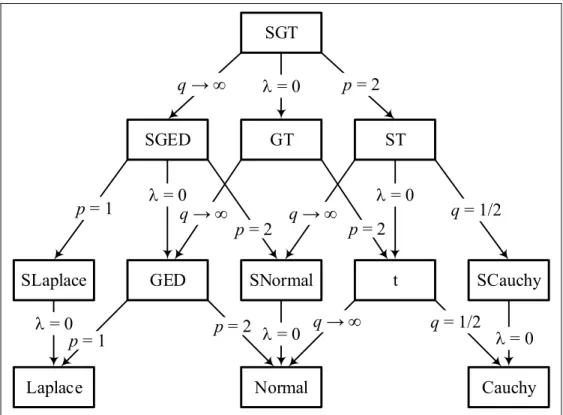
The approach taken for analyzing the stock distribution models was to construct frequency distributions, i.e., histograms, for individual stocks. Preliminary visual evaluation of histograms of the distribution models of a few randomly selected stocks from the stock list implied several candidate distributions: 1) Cauchy, 2) Laplace, 3) generalized-t, and 4) Gaussian.* The more general skewed versions of these distributions were utilized in the analysis to account for any possible asymmetry in the observation data. As developed in [12] and [13], all of these distributions may be derived from the skewed generalized t-distribution (SGT). The SGT t-distribution exhibits a high degree of adjustability and many special cases. Five parameters describe the distribution: , , , p, and q. Figure 1-2 depicts the relationships between the many special cases and identifies the parameter values required to represent any particular distribution.†
* While the Gaussian was visually a poor match for the data, it was included as a reference
due to its widespread historical usage.
SGT GT ST SGED SNormal t SCauchy GED SLaplace
Laplace Normal Cauchy
q → q → q → q = 1/2 q = 1/2 q → p = 2 = 0 p = 1 = 0 p = 2 p = 2 = 0 = 0 = 0 p = 2 p = 1 = 0
Figure 1-2. Skewed Generalized t-Distribution Interrelationships*
The probability density function (PDF) of the skewed generalized t-distribution is defined as
1 1/ ; , , , , 1 2 , 1 1 SGT q p p p p p f y p q p y q q p q sign y , (1-4)* Abbreviations used in the figure: S = Skewed, G = Generalized, ED = Error
where
, is the beta function, p > 0 and q > 0 govern the kurtosis (height and tails) of the density*, is the mean (i.e., location parameter), > 0 controls the variance, and1 1
regulates the skewness. Table 1-1 summarizes the fixed parameters seen in Figure 1-2 that are required for the tested special-case distribution models. By definition, none of the SGT parameters in Figure 1-2 has a fixed value.†
Table 1-1. Summary of SGT Fixed Parameters Cauchy Laplace Normal
p 2 1 2
q 1/2
Thus, the PDF for the skewed Cauchy distribution simplifies to
2 2 2 2 ; , , 2 1 1 SCauchy f y y sign y . (1-5)Additionally, the PDF for the skewed Laplace distribution reduces to
; , ,
1 exp
2 1 SLaplace y f y sign y , (1-6)* Kurtosis increases as p and q decrease resulting in fatter tails, i.e., a leptokurtic
distribution. Increasing p and q reduces kurtosis (possibly yielding negative excess kurtosis), resulting in thinner tails and a distribution that is more platykurtic.
† It may be noted that in the common distribution, also known as Student’s
and the PDF for the skewed Normal distribution is
2 1 ; , , exp 1 SNormal y f y sign y . (1-7)Computations were performed using the R-language version 3.2.5 and the R-Package ‘sgt’ version 2.0. Model optimization was executed with the function sgtmle to identify all five SGT parameters. Function sgtmle fits data to the skewed generalized t-distribution using maximum likelihood estimation and function dsgt was used to compute the model values for each density profile.
1.5.2 Goodness of Fit
After retrieving the input data and preparing the three model sets described in §1.4, a goodness-of-fit measure was computed for each model for each of the 197 stocks in the list. Goodness-of-fit models are used to compare fitted (or theoretical) models with observed data. Several measures for goodness of fit were considered as given in the subsequent five formulas. Note that in the following, yi are the observation values and
*
i
y are the fitted model values. 1. Mean Absolute Error (MAE):
* 1 1 n i i i y y MAE n
(1-8)With MAE, outliers have less influence, but the value is easily understood. There is a disadvantage with noisier data since it places equal weighting on all deviations. 2. Root Mean Square Error (RMSE):
*
2 1 2 n i i i y y RMSE n
(1-9)With RMSE, there is more emphasis or influence by outliers due to the squaring operation. This measure is used often and is an absolute measure.
3. Normalized Mean Absolute Error (NMAE):
* 1 1 1 1 1 1 n i i i n n i i i i y y NMAE y y n
(1-10)This relative measure is used to compare data sets with different scales. 4. Normalized Root Mean Square Error (NRMSE):
*
2 1 2 2 1 1 1 1 n i i i n n i i i i y y n NRMSE y y n n
(1-11)NRMSE, additionally known as the Coefficient of Variation, is also used to compare data sets with different scales.
5. RMSE Normalized to standard deviation ():
*
2 2 2 1 3 2 2 1 1 1 n i i i n n i i i i y y NRMSE y y n
(1-12)This approach is most appropriate and commonly used when the distribution is Normal, since each multiple of σ indicates a percentage of values lying within the band, i.e., 68.3–95.5–99.7%. In the case of non-Gaussian distribution, normalization to σ does not represent these same well-known percentages; however, for a unimodal distribution with a known mode, the Gauss Inequality (also known as the Camp-Meidell Inequality) may be utilized to find associated percentage bands 55.6–88.9–95.1%. (See [14] and Appendix 8.4 for a discussion.)
After preliminary evaluation of some densities, NRMSE (1-11) was selected as the best goodness-of-fit measure for use in the investigation since 1) non-Gaussian densities were evident, 2) there was uncertainty regarding the occurrence of outliers, 3) it was desired to maintain the significance of outliers, 4) normalization was required to compare the diverse price ranges of included stocks, and 5) resulting magnitudes were larger compared to
NRMSE which was the next desirable choice.
For additional assessment, the Cramer-Von Mises (CVM) test was applied as a type of goodness-of-fit test based on the empirical distribution function. The basis of the method is to determine the quality of agreement for an observed sample cumulative distribution
function (CDF) to a hypothesized CDF. The Cramer-Von Mises test statistic for evaluating the null hypothesis H0:X ~ ( )F x , that the distribution X follows a hypothetical distribution F x( ), is defined as [15] [16]
:
2 1 2 : 1 1 2 1 12 2 1 2 1 12 2 n k n k n k n k k CVM F x n n k U n n
, (1-13)where x1:n, , xn n: refers to an ordered random sample of size n, and Uk n: are ordered uniform variables.* The computed CVM statistic value is subsequently compared against a table of critical values, CVM1, to find its corresponding p-value. The null hypothesis,
0
H , should be rejected if CVM CVM1 for an level of significance. It is important to note that the CVM test evaluates a Type II statistical error.† Computations for the Cramer-von Mises test were performed with the function cvm.test available in the R-Package ‘goftest’ version 1.0-3.
* The CVM test of an arbitrary distribution is equivalent to a test of uniformity as
developed in [15] and [16].
† The Type II error is defined as incorrectly retaining a false H0. In other words, there
is a failure to have enough statistical evidence to reject H0, which is in no way equivalent to having strong evidence to support H0.
1.6 Distribution Analysis Results
Each of the four distributions previously identified (skewed versions of Cauchy, Laplace, Gaussian, and Generalized-t) were individually fit to all 197 stocks in the stock list. Moreover, every fit was performed for the daily returns, model residuals, and detrended residuals. For a sense of fits for the various distributions, Figure 1-3 shows an example of stock distributions falling near the average of the range of fit errors.* Clearly, all three sets of observation data have similar types of distributions. The horizontal scales of daily returns and model residuals are very similar, but the horizontal scale for the detrended residuals is much narrower. Inasmuch as all three fluctuation models are normalized, there appears to be less spread, i.e., smaller variance, in the filtered (detrended) model. This is explained by the additional Dn1 term in the denominator of equation (1-3) which reduces the magnitude of the first difference, i.e., the numerator, by approximately two. The vertical axes are set in logarithmic form because a linear scale provided extremely poor visibility for distinguishing between curves. With the logarithmic scale it clear that the Gaussian fit is worst in the tail regions. Corresponding numerical results for Figure 1-3 are given in Table 1-2.
* Note that “Observations” in Figure 1-3 represent conventional histogram bar heights.
Figure 1-3. Typical Example of Distribution Fits 0.01 0.1 1 10 100 -0.3 -0.2 -0.1 0 0.1 0.2 D en si ty Daily Returns Stock: Southwest Airlines (LUV) Observations Skewed Cauchy Skewed Generalized-t Skewed Laplace Skewed Gaussian 0.01 0.1 1 10 100 -0.4 -0.3 -0.2 -0.1 0 0.1 0.2 D en si ty Model Residuals Stock: Southwest Airlines (LUV) Observations Skewed Cauchy Skewed Generalized-t Skewed Laplace Skewed Gaussian 0.1 1 10 100 -0.15 -0.1 -0.05 0 0.05 0.1 D en si ty Detrended Residuals Stock: Southwest Airlines (LUV) Observations
Skewed Cauchy Skewed Generalized-t Skewed Laplace Skewed Gaussian
Table 1-2. NRMSE Summary for Southwest Airlines (LUV)
Daily Returns Model Residuals Detrended Residuals
Skewed Cauchy 0.510 0.374 0.509 Skewed Laplace 0.487 0.344 0.493 Skewed Gaussian 0.411 0.265 0.409 Skewed Generalized-t 0.361 0.150 0.359 -0.001 -0.001 0.000 0.025 0.024 0.012 0.059 0.014 0.034 p 1.786 1.693 1.790 q 3.163 3.815 3.146
The top section of Table 1-2 shows the fit errors for all distributions and fit models for example stock symbol LUV. Lowest errors are in bold. Although all three models were normalized in an attempt to allow comparisons, of principal importance were relative magnitudes within each column. A key result was that the SGT distributions yielded the best fit (lowest error) in all cases. That the SGT showed the best fit was apparent in the curves shown in Figure 1-3 as observations tended to fall on both sides of the SGT curves. It was indisputable that the Gaussian distribution possessed a visibly poor fit as it fell off in the tail regions, which tended to support rejection of normality as noted in other studies. Additionally, the goodness of fit for the Cauchy distribution was limited due to its characteristic fatter tails.
Parameter estimates from maximum likelihood estimation of the SGT distribution are shown in the bottom section of Table 1-2. Mean, , and skew parameter, , were negligibly small, indicating a high degree of symmetry about zero. The value of the variance-control parameter, , was virtually the same for daily returns and model residuals, but was half as large for the detrended model. This discrepancy was previously attributed to the effects of the moving average filter. Parameter values for p and q match closely across all models. With p ≈ 1.76 and q ≈ 3.4, the estimated curve was leaning toward a Student’s t-distribution. A review of the graphs revealed that the optimum SGT fit for all three fluctuation models appeared nearly equidistant from both Laplace and Gaussian distributions.
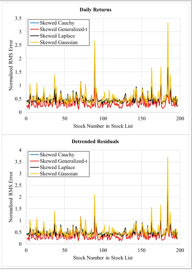
Figure 1-4 shows the normalized RMS errors across all 197 stocks in the stock list for daily returns and detrended residuals. Although not shown, behavior of the model residuals was similar. As a general rule, the SGT distributions yielded the lowest errors. This is seen in the red series in the plots. Also noteworthy was that the Gaussian distributions typically have the highest errors, although there are several exceptions.
Table 1-3 provides the numerical statistics of the normalized RMS errors for the entire stock list for each of the three models. The SGT distribution yielded the lowest errors in every category, as indicated in bold.
Figure 1-4. Normalized RMS Errors Across All Stocks 0 0.5 1 1.5 2 2.5 3 3.5 0 50 100 150 200 N or m al iz ed R M S E rr or
Stock Number in Stock List Daily Returns Skewed Cauchy Skewed Generalized-t Skewed Laplace Skewed Gaussian 0 0.5 1 1.5 2 2.5 3 3.5 4 0 50 100 150 200 N or m al iz ed R M S E rr or
Stock Number in Stock List Detrended Residuals Skewed Cauchy
Skewed Generalized-t Skewed Laplace Skewed Gaussian
Table 1-3. Summary Statistics of NRMSE for All Distribution Estimates Skewed Cauchy Skewed Laplace Skewed Gaussian Skewed Generalized-t Daily Returns Median Mean Max Min Std Dev 0.454 0.508 1.888 0.317 0.185 0.439 0.488 2.414 0.265 0.212 0.460 0.548 3.348 0.230 0.335 0.292 0.341 1.099 0.110 0.169 Model Residuals Median Mean Max Min Std Dev 0.381 0.407 2.029 0.239 0.146 0.356 0.376 2.018 0.164 0.150 0.414 0.465 3.616 0.244 0.291 0.174 0.204 0.701 0.054 0.108 Detrended Residuals Median Mean Max Min Std Dev 0.458 0.509 2.227 0.316 0.187 0.446 0.491 2.303 0.269 0.194 0.466 0.547 3.698 0.229 0.332 0.306 0.351 1.264 0.134 0.177
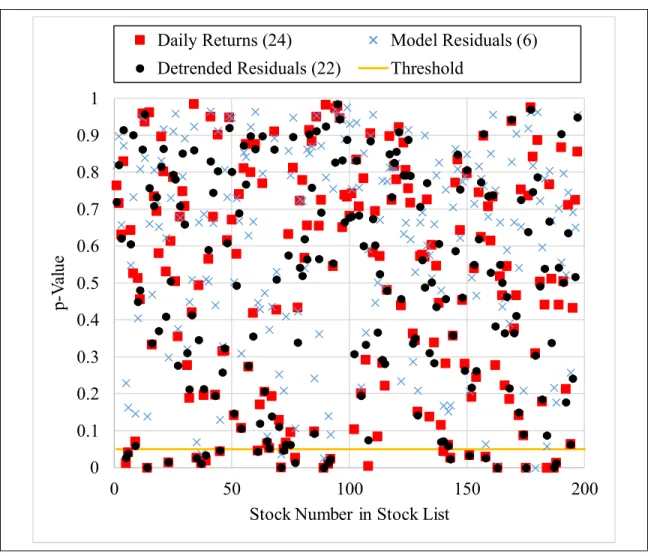
A graph of results for the second goodness-of-fit evaluation using the Cramer-von Mises test is shown in Figure 1-5. The frequency of occurrence (count) for values less than the significance level (threshold = 0.05) are given in the legend for each model. These computed to approximately 12%, 11%, and 3% for daily returns, detrended residuals and model residuals, respectively. Overall, there was good agreement that most of the stock distributions (≈ 90%) were accurately classified as generalized t-distributions.
A summary of the statistics of the estimated parameters is given in Table 1-4. Parameters , , and were consistent with characteristics mentioned for the example stock LUV. Parameter p ≈ 1.64 for the daily returns and detrended residuals and was slightly lower at 1.58 for the model residuals, all similar to the LUV example. The median of parameter q ranged from 2.66 to 2.94, while the mean was quite variable due to some extreme values. Overall, there was a high degree of consistency for each model across the array of stocks.
Figure 1-5. p-Values for Empirical CDF Goodness-of-Fit 0 0.1 0.2 0.3 0.4 0.5 0.6 0.7 0.8 0.9 1 0 50 100 150 200 p-V al ue
Stock Number in Stock List
Daily Returns (24) Model Residuals (6) Detrended Residuals (22) Threshold
Table 1-4. Summary Statistics of Parameters for All Distribution Estimates p q Daily Returns Median Mean Max Min Std Dev 0.000 0.000 0.001 -0.002 0.001 0.017 0.018 0.039 0.0005 0.005 0.028 0.027 0.089 -0.045 0.021 1.639 1.622 2.698 0.345 0.314 2.662 386.9 33408.4 0.860 2800.3 Model Residuals Median Mean Max Min Std Dev 0.000 0.000 0.001 -0.001 0.000 0.017 0.018 0.037 0.006 0.004 -0.003 -0.005 0.027 -0.065 0.016 1.584 1.576 2.576 0.572 0.255 2.942 338.6 22890.0 0.926 2695.9 Detrended Residuals Median Mean Max Min Std Dev 0.000 0.000 0.001 -0.001 0.000 0.009 0.009 0.019 0.002 0.002 0.013 0.009 0.071 -0.602 0.048 1.647 1.625 2.701 0.675 0.310 2.665 435.1 25197.5 0.614 2604.8
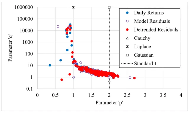
Figure 1-6 shows a graph of the p-q relationships of the parameter estimates for each model for each stock. Clearly, most of the estimates fell in the range of 1 p 2.7 and 0.9 q 10. It is rather deceiving that the estimates fall closest to the Cauchy distribution in Figure 1-6 in contrast to the example of Figure 1-3 which shows the Laplace distribution as a better visual match to ( , ) (1.76,3.4)p q . Of course, some data points fell on the standard t-distribution (vertical) line. Evidently, the SGT model has a substantial sensitivity to p and q values with respect to distribution tails.
Figure 1-6. Parameter Estimates
1.7 Summary of Stock Characteristics
The evidence from analyzing approximately forty percent of the stocks in the S&P 500 resulted in a strong rejection of the assumption of Gaussian distribution of major U.S. equities. Studied stock data belonged to the category of large market capitalization (large-cap) and spanned over 25 years. Distributions of daily stock returns, model residuals, and detrended residuals all showed fat tails and high peaks as displayed in the example histogram of daily returns in Figure 1-7 (using a linear vertical scale)*. The alternative distributions of Cauchy, Laplace, and Gaussian all resulted in poorer fits than the Generalized-t model. Skewness and mean offsets were found to be negligible.
* This is the same observation data shown in Figure 1-3.
0.1 1 10 100 1000 10000 100000 1000000 0 0.5 1 1.5 2 2.5 3 3.5 4 P ar am et er 'q ' Parameter 'p' Daily Returns Model Residuals Detrended Residuals Cauchy Laplace Gaussian Standard-t
Figure 1-7. Typical Example of Non-Logarithmic Histogram Scale 0 10 20 30 40 -0.3 -0.2 -0.1 0 0.1 0.2 D en si ty Daily Returns Stock: Southwest Airlines (LUV) Observations
2. STATISTICAL FORECASTING OF TIME SERIES “Probability is expectation founded upon partial knowledge.”
– George Boole (1815-1864), in the book “Collected Logical Works,” vol. 2, 1940
This chapter addresses an investigation into the forecasting of stock time series based on statistical methods. All of the concepts and definitions introduced in Chapter 1 are applicable here as well. In addition to computing forecasts, their accuracies must be specified and this is expressed with probability limits, i.e., confidence intervals, on each side of a forecast value. While any convenient limits may be used, 95% confidence intervals (CI) are utilized in this investigation. In other words, there is a 95% probability that a realized value will occur within the CI limits.
The study compares the results of statistical forecasting of univariate time series to multivariate time series. Forecasting methods are applied to a time series, Zn, assuming that the time series can be modeled as a stochastic process with an identifiable form. The paradigm used is the very general autoregressive integrated moving average (ARIMA) model. The hypothesis investigated is whether a multivariate time series of correlated stocks produces better forecast results than a single (univariate) series alone.
2.1 Analysis Approach – Windows and Splits
Each stock series examined spanned a range of 25 years of daily samples for a total of 6491 data points. To obtain independent statistics, a stock time series was divided into non-overlapping windows of 100 samples each*. This generated 64 completely independent sample windows for each stock. Analyzing 100-sample windows avoided any seasonal or repetitive cycles within or between windows that may have occurred over the data span of 25 years. One-hundred sample windows also provided a sufficient set of training data to establish an adequate model.
Stock time series have two unique aspects that separate them from naturally-occurring or scientifically-based time series: splits and ex-dividend days. A stock split causes no change in a shareholder’s portfolio value nor in a firm’s asset value. The occurrence of a split appears as a noticeable instantaneous shift in the time series pattern at some specified date.† For securities in the stock list, splits typically occurred 3-5 times over the 25 year data range. A split was managed as follows. For each stock, split dates and corresponding split ratios were obtained from Yahoo! Finance via the getSplits function in the R-Package ‘quantmod’ version 0.4-5. If a stock splits on day n with ratio r, e.g., a 2-for-1 split returns r = 0.5, then all price data in the window prior to day n are multiplied by r.‡ Implementing this adjustment produces a price time series without the large shift, providing continuity
* One hundred daily samples correspond to approximately 4.75 calendar months. † Examples can be seen as vertical price changes in Figure 1-1.
for model building. On the other hand, the processing of any dividend payout on a stock was ignored and considered insignificant for this study.
2.2 Univariate Analysis
To analyze the univariate time series, computations were performed in the R language employing the auto.arima function from the R-Package* ‘forecast’ version 6.2. The auto.arima function returns the best-fit ARIMA model when evaluated against the Corrected Akaike Information Criterion (AICC), by searching over all possible models within specified model order constraints. The search range for model order was limited to a maximum of 5 for p and a maximum of 5 for q.
Univariate ARIMA Model
The ARIMA model combines the autoregressive (AR) and moving average (MA) models with differencing, also known as the integrated (I) component. Differencing parameter d specifies the number of first differences applied to the series to achieve stationarity. Some noteworthy models are identified in Table 2-1 [17].
Table 2-1. Special ARIMA Models
Name Model
White Noise ARIMA(0,0,0)
Random Walk ARIMA(0,1,0) with no constant Random Walk with Drift ARIMA(0,1,0) with constant
AR(p) ARIMA(p,0,0)
MA(q) ARIMA(0,0,q)
A time series is required to be stationary in order to produce a proper model estimate. If the model is estimated in the presence of any non-stationary parameters, the estimated coefficients may be incorrect. Differencing makes the time series stationary. The number of required differences can be determined by checking for unit roots. In the auto.arima function, the Kwiatkowski–Phillips–Schmidt–Shin (KPSS) unit-root test was used.*
The non-seasonal ARIMA(p,d,q) model† is defined as
B 1 B
d yt c
B t , (2-1)
where
z is the AR polynomial of order p and
z is the MA polynomial of order q, B is the backshift operator,
t is a white noise process with zero mean and variance2,
and c is a constant. Equation (2-1) may be expanded as
* In the KPSS test, the null hypothesis is stationarity and the alternate hypothesis is a unit
root, i.e., a non-stationary process.
11BpBp
yt c
11BqBq
t , (2-2)which may restructured into the predictive form as
1 1 1 1
t t p t p t q t q t
y c y y . (2-3) It is clearly seen in equation (2-3) that predictors include lagged values of yt and lagged error terms of t.
The auto.arima function cycles through various combinations of (p,q) model orders. After selecting a model order, estimation of parameters c, 1, …, p, 1, ..., q is performed using maximum likelihood estimation (MLE). Maximization is accomplished via the AICC, defined as [18]
2 1 2 2 p q k p q k AICC AIC T p q k , (2-4)where the Akaike Information Criterion (AIC) is
2ln( ) 2 1
AIC L p q k , (2-5)
and L is the likelihood of the data*, T is sample size, k 1 if c0, and k0 if c0. The (p,q) model, with estimated parameters, associated with the optimum AICC value is the final selected model.
* The likelihood is calculated with the arima function in the R-Package ‘stats’, which
computes the exact likelihood using a state-space representation of the ARIMA process, and the innovations, i.e., errors, and their variance are found via a Kalman filter.
Forecasting characteristics of ARIMA models depend on the values taken by parameters c and d in the above formulas. Table 2-2 lists the expected performance traits [17]. Additionally, as parameter d increases, the size of forecast confidence intervals increase as well. On the low end, when d 0, the forecast standard deviation tends to the standard deviation of the historical (training) data. Interpretation of the long-term forecasting behavior of ARIMA models (Table 2-2) infers convergence to the data sample mean. This implies that the utility of stationary models is principally for short-term predictions.
Table 2-2. ARIMA Model Forecasting Behavior
c d Long-Term Forecast
0 0 Tends to zero
0 1 Tends to a non-zero constant 0 2 Follows a straight line
≠ 0 0 Tends to the mean of the data ≠ 0 1 Follows a straight line
≠ 0 2 Follows a quadratic trend
2.3 Univariate Results
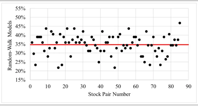
Results of applying the auto.arima function yielded a maximum model order of 4 for parameters p or q across all windows of all stocks. In contrast, the frequency of occurrence of random-walk models, ( , , ) (0,1,0)p d q , seen in Figure 2-1, was prominent, ranging
from 43 to 77%, with a mean of 63% (indicated by the red line).* All random-walk models occurred with a first difference in the analyzed time series. From the properties of a random walk, the forecast for a model without drift is simply a horizontal projection attached to the last observed sample, while a model with drift may project along a sloped path up or down from the last observation. While actual stock price movements have reasons for moving as they do,† the implication of the random-walk model is that forecast direction and magnitude cannot be predicted. Hence, a random-walk model is ineffective for producing useful forecasts. Fortunately, random-walk models, although frequent, did not occur in every sample window.
Figure 2-1. Frequency of Univariate Random-Walk Models
* Drift may or may not be present. Note that a random-walk model with drift indicates
that the distribution of step sizes has a non-zero mean as opposed to no drift equating to a zero mean.
† Although beyond the scope of this work, there are many theories regarding stock price
movement. To encapsulate, a stock’s change in price is not random, without purpose, but may sometimes be explained subsequently.
40% 45% 50% 55% 60% 65% 70% 75% 80% 0 25 50 75 100 125 150 175 200 R an do m -W al k M od el s Stock Number
It is generally believed that a well-fit ARIMA model exhibits a lack of serial correlation within the model’s residuals [19]. While it is a common practice to use the Ljung-Box portmanteau test [20] for evaluating serial dependence, no theoretical basis has been developed for identifying the proper number of lags for the test [21]. For T data points, Hyndman [22] recommends using l lags where lmin 10,
T / 5
. Since Ljung and Box published their test approach in 1978, alternative tests with more power have been developed [23] [24]. While the Ljung-Box test is time-based, these alternate tests are based in the spectral (density) domain and perform better on both Gaussian and non-Gaussian distributions, with only small loss of power. Normality of stock data is clearly absent as established in §1.6, and therefore any test must have the ability to verify serial correlation for non-Gaussian distributions.To establish the reliability of the forecasting analyses, serial correlation tests were performed on the model residuals for all stocks in all windows using both the Ljung-Box portmanteau test and the test statistic, Tn, developed in [23]. The Ljung-Box test is implemented in the function Box.test in the R-package ‘stats’* and the spectral density test for Tn is implemented by the function UnivTest in the R-package ‘dCovTS’ version 1.0. The Ljung-Box test was executed with a lag of 10 and degrees of freedom equal to ARMA
model order p q . The correlation Tn statistic was computed utilizing a Daniell smoothing window,* bandwidth = 10,† and number of bootstrap replicates = 499.
Results of the serial correlation tests are shown in Figure 2-2. The top graph refers to the Ljung-Box test results and the bottom plot refers to Tn test results. Both scatterplots show for each stock the proportion of p-values (out of 64 windows) that are below the threshold of 0.05 (shown as a red line). With a null hypothesis of independence, a small p-value expresses strong implication against independence, rejecting the null hypothesis. Thus, if a stock displays a small fraction of p-values below 0.05, then the hypothesis of independence is accepted. The Ljung-Box results indicated 55 out of 197 stocks rejecting the null hypothesis, whereas the spectral density statistic, Tn, rejected only two. These two (PEP and VZ) were recomputed with the Daniell kernel and again found to have four windows with p-values less than 0.05 as displayed in Figure 2-2. As seen in the figure, the fractions appear in discrete jumps since they are increments of 1/64. Results for stocks PEP and VZ produced a fourth window where the p-values were below 0.05, pushing them over the 0.05 threshold. Any window with a low p-value may be interpreted as having a model fit that is less than the best possible since some serial correlation of residuals remains, but this does not invalidate its model. Inasmuch as the Tn statistic has
* The computational time of the Daniell window was costly, but produced more accurate
results (according to [23]). A Bartlett window was also run, yielding results showing no serial correlation for all stocks.
demonstrated higher power [23], all models were accepted as independent and not serially correlated, validating the ARIMA model fits.
Figure 2-2. Serial Correlation p-Values for Univariate Model Residuals
Accuracy of forecasting direction of movement was found by comparing one-step ahead and five-step ahead predictions with out-of-sample data. Results of directional forecast accuracy for each stock are displayed in Figure 2-3 and summarized in Table 2-3. A 50%
0 0.05 0.1 0.15 0.2 0 25 50 75 100 125 150 175 200 L ju ng -B ox p -V al ue < 0 .0 5 Stock Number 0 0.01 0.02 0.03 0.04 0.05 0.06 0.07 0 25 50 75 100 125 150 175 200 S pe ct ra l D en si ty p -V al ue < 0 .0 5 Stock Number
threshold represents a type of result from a random occurrence, meaningless for effective forecasting. Results above (or below) the 50% threshold provide an improvement to a random guess, either forecasting the correct direction of movement, or forecasting incorrectly the direction of movement.* Table 2-3 also includes the number of occurrences for which the sign of forecast directional accuracy was the same for both one-step and five-steps ahead. In other words, if both the one-step and the five-step forecast were both greater than 50% or both less than 50%, that stock was counted in the total for being in the same direction. This may provide a stronger indication of expected directional movement.
Figure 2-3. Univariate Directional Forecast Accuracy
* It may also be useful for trading to recognize (with some probability) that a forecast
direction is incorrect. 35% 40% 45% 50% 55% 60% 65% 0 25 50 75 100 125 150 175 200 A cc ur ac y Stock Number Ahead 1 Ahead 5
Table 2-3. Univariate Directional Accuracy Summary Forecast Interval Accuracy Frequency (Out of 197)
Ahead 1 > 60% 2 > 55% 24 > 50% 93 < 45% 8 < 40% 0 Ahead 5 > 60% 1 > 55% 18 > 50% 93 < 45% 22 < 40% 2
Ahead 1 & Ahead 5 Same Direction 111
Coverage refers to the percentage of forecasts that fall within a confidence interval. For each forecast window of each stock, the one-step- and five-steps-ahead forecasts falling within the 95% confidence interval were counted and the fraction of total windows was computed. Results are displayed in Figure 2-4. The results were greater than 82% for all stocks, with the average for one-step ahead at 92.5% and for five-steps ahead at 92.8%.
Figure 2-4. Univariate Forecast Coverage within 95% CI
2.4 Multivariate Analysis
Multivariate analyses were performed on pairs of correlated stocks. Vector time series models were estimated utilizing the R language and a modified* version of Tsay’s [25] VARMA† function available from the R-Package ‘MTS’ version 0.33. Each time series (100-sample window) was initially made stationary by differencing via the ndiffs‡ function available in the R-Package ‘forecast’ version 6.2. Search range for model order was limited to 0 p 2 and 0 q 2, resulting in nine models computed for each multivariate series
* Any function described as a “modified” version connotes that the essential elements of
the original function were retained, but that unused lines of code were eliminated.
† VARMA is the abbreviation for Vector Autoregressive Moving Average.
‡ As in the univariate case, the KPSS test was applied as the unit-root test to determine
the number of differences to reach stationarity. Computational results yielded a difference value of either zero, one, or two, for any window.
80% 82% 84% 86% 88% 90% 92% 94% 96% 98% 100% 0 25 50 75 100 125 150 175 200 C ov er ag e Stock Number Ahead 1 Ahead 5