Forecasting Model of Electricity Demand in the Nordic Countries

(1)

Forecasting model of

electricity demand in

the Nordic countries

Tone Pedersen

(2)

1

Abstract

A model implemented in order to describe the electricity demand on hourly basis for the Nordic countries. The objective of this project is to use the demand data simulated from the model as input data in the price forecast model, EMPS model, at Vattenfall. The time horizon is 5 years, 6 years including the current year. After different models tried out, the final model is described by fundamental and autoregressive time variant variables, an ARX model. The variable of temperature is described by historical data from 46 years which are used to create an idea of the outcome variation depending on the weather. Non parametric bootstrap of the residuals is used when adding noise to the simulation. The ARX parameters was estimated by prediction error method but a two-step estimation was also tried, by first estimating the fundamental parameters and then model the rest of the demand by an AR process. The second method was supposed to increase the weight on the fundamental variables. Results of the simulation Indicates of a realistic description of the electricity demand which is an improvement of the earlier demand input to the EMPS model but the difference is not always seen in the outcome of the price forecast. The results are discussed in Chapter 5.

(3)

2

Acknowledegements

I would like to thank my supervisor at Vattenfall, Anders Sjögren, and specially Roger Halldin at Vattenfall for all his help and guidance throughout this thesis. I would also like to thank Björn Wetterberg at Vattenfall and my examiner at Lund University Erik Lindström.

(4)

3

1. Introduction

1.1 Background

This master thesis is a project for Vattenfall AB and the business unit Asset optimization Trading, AOT . Vattenfall is one of the biggest energy companies in Europe where one of its main tasks is to produce and sell electricity to a profitable price.

In order to maximize the revenue it is important to have a good price prognosis. The MA/ seasonal planning department is the department that is in charge of the price prognosis of the next five year. The MA/Seasonal planning is using a forecast price model, the EMPS model, or EFI as it is called internal in Vattenfall. The EMPS model is taking into consideration input parameters as such consumption, transmission capacity water values (which are computed in the system), fuel prices, etc.

1.1.1 EMPS model

The main purpose of the EMPS model is to forecast the spot price in deregulated markets. The price is evaluated by considering estimation of the water values and the input data provided by the user.

The EMPS model of Vattenfall, called EFI, is a forecast of the next five years, six including the current year, electricity price with a weekly resolution.

The EMPS model has two steps in its procedure. The first part, called the strategy part, develops the water values. In the second part the system uses the water values and the input data from the user to simulate the output. The output consists of water values for water power stations, prognosis to the Nordic system price, the price areas, the power production and reservoir development.

EMPS is a model created to optimize and simulate the hydropower system. It takes the transmissions between different regional reservoirs and between bigger areas into consideration. The system uses the flexibility in the hydropower system to stabilize future uncertain inflows which are less steerable or non-steerable. The hydropower is optimized in relation to regional hydrological inflows, thermal generation and power demand.

The steering of the hydropower is done by computing water values for each region. A high water value indicates a lower water level/volume in the reservoir. The water value is computed by a stochastic dynamic programming where also the interaction between the areas are included. Optimal operational decisions are evaluated for each time step for thermal and hydro production. This is done by considering the water value of the aggregated regional subsystems. In each subsystem a more detailed plan of the distribution of the production is done according to the number of plants and reservoirs.

(9)

8

In the EFI model, the price is simulated with 46 different weather scenarios, actual historical weather years. The scenarios are used in blocks of five years to include an actual historical 5 years weather change.

The existing EMPS model simulates the 46 simulations 5 times per week which will expand to 168 times per week if the model will be transformed to an hourly based model. An update of the EFI model with 84 times 46 simulations per week is done but not jet implemented due to non-updated input data.

1.1.2 What is the need of a demand forecast on an hourly basis?

Over the years the renewable energy sources wind and solar power have rapidly increased. The sources are obviously only producing when there is wind or sun which is why these renewable sources cannot be a base energy source, a source to rely on. When wind or solar power or both are producing a lot of energy they also increase the supply on the market. The supply and demand curves of the electricity market will meet at a lower electricity price. If the wind and solar power would produce a constant amount of electricity during specified periods the electricity spot price would not be hard to forecast. This is where the time resolution becomes a problem for the model. The wind and solar power are only producing when there is wind or solar which is sometimes hard to forecast and can change quickly during a day. This results raises the volatility in the electricity price during the day. Because the price forecast is set on a weekly basis the daily high and low peak prices will not be caught in the model. The information that is lost makes the model output lose its momentum.

In order to catch the momentum during the day and improve the resolution of the output data, the input data must contain information on the same time scale basis as the output data that is on an hourly basis. One of the input data to the model is the electricity demand forecast for the next 5 years. The demand data is today on a monthly basis which is added together to annual data, the price model is then distributing the demand data over the year on an two hourly basis. The system has a daily, weekly and yearly profile of the consumption which is used when distributing the monthly consumption data.

1.1.3 Background of the electricity demand

Parts of the electricity consumption are static processes in form of the consumption of the households and the consumption of lighting. This part is relatively easy to model since it is not affected by unexpected events. The households consumption of electric heating during the winter is closely related to the temperature. When the temperature is very low then the electric heating stagnates, meaning it does not increase more. Electricity consumption versus temperature is deferring depending on if you are in southern, middle or in northern Europe. The difference is due to the use of air condition in southern and middle Europe. As the air condition uses as much electricity as the electric

(10)

9

heating the electricity consumption is higher in southern and middle Europe than in northern Europe. In the north the temperature related electricity consumption could be omitted during summer.

Another part of the electricity consumption is the electricity consumed by the industry. The industry looks very stable on a daily basis but looking at a long run perspective the industry production varies with the economic cycle. If the economic situation is falling the situation in the country will worsen and some industries will have difficulties to survive, these might therefore decrease the production and in worst case shut down their industry. This part is hard to model since it needs to be observed from many perspectives and deeper investigation is needed to detect the industries that will disappear. Because of this it was decided to use the already existing demand forecast on a monthly basis where investigation and previous knowledge is creating the forecast.

The model should partly be based on analyses of these factors and analyses of other possible contributing factors.

1.1.3.1 Previous models used within electricity demand

The electricity demand, is a quite well investigated area where most of the models have a time horizon of either intraday, one week, one year or long term as 10 years ahead. Speaking of general modeling of electricity demand, the traditional techniques of forecasting are regression, multiple regression, exponential smoothing and iterative least squares techniques (Singh, Ibraheem, Khatoon, & Muazzam, 2013). The range of models are varying between manual methods that has been tested operationally and formal mathematical approaches. (BOFELLI & MURRAY, 2001)

The most popular model is the multiple regression model which is describing the demand by a number of factors that are affecting the electricity demand in different ways (Singh, Ibraheem, Khatoon, & Muazzam, 2013). The interest of load forecasts is typically aimed to the hourly quantity of the total system load. (Alfares & Nazeeruddin, 2002)

The development of the traditional methods has modified the previous techniques by keep track of the environmental changes and update the parameters during the forecast along with the changes. The most popular model among the modified technique is the stochastic time series methods. The time series models are looking for internal structures such as seasonal trends and autocorrelation.

All models tried out are more or less imprecise and uncertain due to the fact that there are unknown or totally random variables. Instead of using hard computing, trying to find the exact solution, soft computing solution has over the last few decades been used. The soft computing is using the environment of approximation rather than being exact. (Singh, Ibraheem, Khatoon, & Muazzam, 2013)

(11)

10

Looking at the chronological order, the ARMAX model is found straight after the stochastic time series. As many of the popular models are best suited to short term load forecasting this model has also been tried out on long term where the result was compared with regression methods. (Alfares & Nazeeruddin, 2002) Another technique that has been used within the electricity demand model is the dynamic factor model which can be modified in several ways. (Mestekemper, 2011) It is briefly explained as reducing the dimension of the original set of data which gives e.g. better parameter estimation. The method is mostly used when the time horizon is short. See appendix B for further reading.

1.2 Purpose

The main purpose of the model is to describe the electricity consumption during the days depending on what weekday it is, if it is a public holiday or an expected vacation day. The model should also be able to observe how the electricity consumption is varying depending on the temperature input. The model should also be able to change the pattern while the input data is being updated and explain future year’s consumption.

The idea of the project is to improve the model of the consumption data used for the EMPS model with an hourly resolution by systemizing it and increasing the quality and reliability of the model, compared to today’s monthly consumption data. The outcome of the project is an implemented model where the output is forecasted hourly consumption for the next five years. The main focus in the model is to create a normal consumption year and then use the monthly forecasted consumption, from the consumption model that is used for the EMPS model today, to profile the future years. The model should be implemented and calibrated for each of the Nordic countries separately.

The path of the project includes investigations of different models and to find a suitable definition of the demand. Different variables were tested to conclude what is affecting the electricity consumption. The analysis of the observed consumption is investigated mostly by time series analysis and several time series models have been investigated for a possible fit. Static models have also been tried and by then combinations of stochastic processes based on regression models was also included.

In order to handle the noise added to the model I used block bootstrap and tried different ways to identify the periods of the more significant noise.

The simulation was tested out by different methods, e.g. prediction with different time horizons. The final method was to use prediction with one time step as time horizon and then add noise. This was executed for each time point and continued until the timeline of the simulation was outlined.

(12)

11

1.3 Limitations

Included in the specification when I started the project was to be able to see the trends in the price if the electricity consumption was distributed differently during the day. The goal was to see the change in price if the consumers was affected by the information available in order to consume the electricity when the price was lower during the night.

There is no trend seen when looking at historical data which means that the data has to be created by modification of the real data. A possible way of create this data is to investigate the behavior within peoples habits and what would be a possible future scenario of the consumption. This investigation would need a lot of information analyzed and this was too time consuming.

Another aspect of the project that had to be removed from the scope was to modify the economic growth of the year more precisely. The idea was to identify the industrial consumption since the factories is the group which is most affected of an economic national change. If the economic growth goes down a lot of factories has to decrease their production and worst of all shut down. And the other way around if the economic situation will improve. In order to identify the industrial consumption in the northern countries a lot of data had to be found to identify the factories. The simplified solution was to modify all the consumption which still gives a better way to describe the consumption than the outcome data used before.

1.4 Result

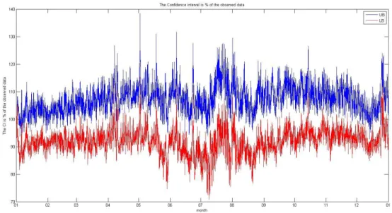
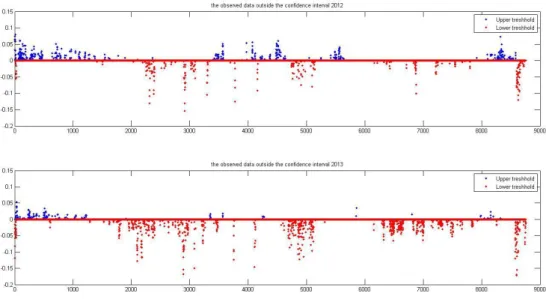
The main result of this master thesis shows that the model developed captures the annually, weekly and daily trends. It also follows the changes in the temperature very good. With the noise added and with 46 weather scenarios as temperature input data the 95% confidence interval gives has a relatively good spread. The validation of the spread is done by calculating the amount of observed demand hours which is outside the confidence interval which is slightly above 5%. 5% would be approved as it might be in the quantiles of the 95% confidence interval.

Another objective was to use the demand model to simulate input data to the EMPS model. The result showed that the more specific hourly model improved the variation from day to night during the summer period. There is hardly any significant changes in the spring period, some days have more variations from day to night others are the same as with the old demand data.

1.5 Outline

This thesis is structured into 6 sections. It starts with an introduction about the EMPS model and why this project was set up. Section 2 is handling the theory needed to know to understand the modeling part and some of the result section. The theory can be read with varied carefulness depending on the mathematical background. This section is mostly describing and defining methods used within

(13)

12

time series analysis but also describes bootstrap which is used when simulating the model. The modeling part, section 4, is guiding the reader through the way taken to arrive to the ARX model which was chosen. Section 4 is also showing the method used for simulating the model. The modeling section is followed by the results which is mostly analyzing the result of the demand model. The section concludes with result from the EMPS model, if the change from demand on annually basis to hourly basis had an impact on the price and how the noise added to the demand data was seen in the price. The last section is discussing the results and also give some tips of future work.

(14)

13

2. Theory

This part contains the theory behind the tools that has been used to conclude the best model solution. The final model is structured by a time series model with deterministic input variables that are effecting the electricity consumption in a one way relation. Meaning e.g. the electricity demand would change if the temperature changed but the temperature would not be effected if the electricity consumption changed.

2.1 Time series analysis

A time series { } is a realization of a stochastic process

{ }.

DEFINITION 1 Stochastic process

The process { } is a family of random variables { ( )} where t belongs to an index set.

Time series analysis are statistical methods, e.g. time series models, that are often used to model physical events as stochastic processes.

The stochastic process has two arguments{ ( ) }, ( ) is a random variable for a fixed t and is the sample space on the set of all possible time series, , that can be generated by the process.

The stochastic process described must have an ordered sequence of observations. The ordered sequence of observations is the order through time at equally spaced time intervals. (Madsen, Time Series Analysis, 2008)

The model used can be seen as tools often used when it is hard to describe all patterns by deterministic variables or there are no fundamental parameters at hand. The time series models finds the underlying forces by observing the correlation between previous and current data points. The linear time series models are constructed by either autoregressive parameters or a moving average parameters, or a combination of these two. The autoregressive parameters is looking after a lagged correlation between the current data point and previous data points. The moving average is looking after the correlation in the residuals that is deviating from a mean of all data points.

Two linear processes that are the base for time series models are the Moving average process, MA process and the autoregressive process, AR process which are defined as follow

DEFINITION2The MA(q) process The process { } given by

(15)

14

Where { } is white noise, is called a Moving Average process of order q. In short it is denoted an MA(q) process.

DEFINITION 3 The AR(p) process The process{ } given by

(2.2) Where { } is uncorrelated white noise, is called an autoregressive process of order p (or an AR(p) process).

(Madsen, Time Series Analysis, 2008)

2.1.2 Time series models

In the following part, the theory of the models I tested will be described shortly just to be sure that reader understand section 3, the modeling part.

2.1.2.3 ARMA

Auto regressive moving average process has the following equation DEFINITION4 The ARMA(p,q) process

The process { } given by

(2.3)

Where { } is white noise is called an ARMA(p,q) process.

2.1.2.2 SARMA

SARMA, Seasonal Autoregressive moving average process, removes the seasonal pattern from the data sequence before fitting the data to the ARMA model.

DEFINITION 5 Multiplicative ( ) ( ) Seasonal model

The process { } is said to follow a multiplicative ( ) ( ) seasonal model if

( ) ( ) ( ) ( )

(2.4)

Where { } is white noise and are polynomials of order and , respectively, and and are polynomials of order and , which have all roots inside the unit circle.

The method of seasonal adjustment is used to capture the underlying trend which becomes more distinct when removing the seasonal trend. Long term forecasting is less suitable for seasonal models as they are adapt for non-stationary data which is hard to forecast in long term. More reading will follow in section 3.1.1.

(16)

15

2.1.2.1 SARIMA

The SARIMA, seasonal autoregressive integrated moving average process differentiates the data by both considering the seasonal periodic pattern of order D and differentiating afterwards the data by order d to become stationary. After filtering the data by the seasonal differentiation the model structure will be easier to identify by ACF and PACF. The equation of SARIMA looks like,

DEFINITION 6 Multiplicative ( ) ( ) Seasonal model

The process { } is said to follow a multiplicative ( ) ( ) seasonal model if

( ) ( ) ( ) ( )

(2.5)

Where { } is white noise and are polynomials of order and , respectively, and and are polynomials of order and , which have all roots inside the unit circle. (Jakobsson)

This seasonal method is hard to use when the focus of the model should be on the seasonal pattern and not only to find the underlying factors. This is the same issue as in 2.1.2.2.

The other problem with SARIMA is that it is integrated one time which means in this case that it has been differentiated. The differentiation also makes it difficult to go backwards since it is only the difference between the data points that is used when the model is done.

2.1.1 Identification of the model and model order

The identification of the model is based on the stochastic process found in the data. The data modeled is one or more time series. To be able to describe a stochastic process with a time series model the process has to be stationary. DEFINITION 7 weak stationary

A process { ( )} I said to be weakly stationary of order k if all the first k moments are invariant to changes in time. A weakly stationary process of order 2 is simply called weakly stationary. (Madsen, Time Series Analysis, 2008)

One of the primary tools for time series analysis is the estimation of the correlation.

2.1.1.1 ACF – autocorrelation function

DEFINITION 8 Autocovariance function

The autocovariance function is given by

( ) ( ) [ ( ) ( )] [( ( ) ( ))( ( ) ( ))] And the autocorrelation function is given by

(17)

16

( ) ( ) _√ ₍( ₎ ₍) ₎ (2.6) The time series is from start at least or is integrated to become weak stationary before continuing the modeling. If the time series is stationary the autocorrelation function will be a function of the time difference

( ) ( ) ( )

( ) _(2.7)

The difference from the earlier equation is that the variance is the same no matter of where in the process you are. For example ( ) =

due to the variance should be equal in all time steps.

To investigate which model structure that is appropriate to describe the data the autocorrelation function, ACF is a good way to start with.

As defined above the autocorrelation function is a description of the relation between the covariance of two data points and the variance of the process. The output is the correlation between the data from different time steps in the process.

To identify if the process is a pure AR process, autoregressive process, or a pure MA process, moving average process the following theorem will show what to be observant of.

THEOREM 1 Property for AR processes

For an AR(p) process it holds

[ ̂ ] (2.8)

[ ̂ ] (2.9)

k=p+1,p+2,…

where N is the number of observations in the stationary time series and is the PACF.

The ACF of the AR process has the characteristics as a damped exponential and/or a sine function.

THEOREM 2 Property for MA processes

For a MA(q) process it holds

(18)

17

[ ( )]̂ [ ( ̂ ( ) ̂ ( ))] (2.11)

k=q+1,q+2,…

where N is the number of observations in the stationary time series and ( ) is the ACF.

The orders of the pure processes can be observed by looking at the estimated variables ( )̂ ( ) and ̂ ( ) , which should be approximately normally distributed. For example the ̂ is approximately zero after the order p since there are no correlation in the current time step and the delays further on. If the process is mixed, there are both MA and AR processes within the stochastic process, the model order is far more difficult to discover where the trial and error method is useful. Different orders are tried out until no significant lags are seen. (Madsen, Time Series Analysis, 2008)

The right model order is found when the parameters of the Sample Autocorrelation Function, SACF, no longer are significant except of k=0 which will always be 1 since it is the variance divided by itself. SACF is the autocorrelation function of one sample. (Madsen, Time Series Analysis, 2008)

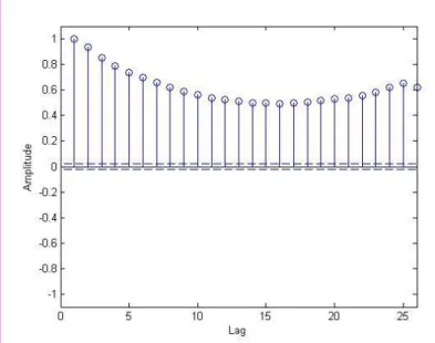
Figure 1 The autocorrelation function when there is a correlation between current data point and the data point in time point 25. This is a pure AR process since it has the form a sine function.

When analyzing the residuals after a simulation theorem 3 can be used to see if the simulation is simulating correct.

DEFINITION 9 The inverse autocorrelation function

The inverse autocorrelation function (IACF) for the process

, {

},

is found

as the autocorrelation at lag

k

is denoted

( )

(19)

18

THEOREM 3 Inverse Autocorrelation function for AR processes

For an AR( ) process it holds that

( ) (2.12)

( )

PROOF Follows from the fact the at the AR(p) process, ( ) , can be written as ( ) if is stationary.

2.1.1.2 Optimization of the number of parameters and model

order

The following methods are used in order to validate the model order and also to see if the number of parameters is optimized.

The loss function is using the residual sum of squares, RSS, and is comparing the RSS for different number of parameters in order to see when the number of parameters is optimized. The RSS is written as

∑( _{̂ ̅)}

∑_{( ̅)} (2.13)

The RSS gives information of the proportion of the variation explained by the model compared to the total explained variation in y. (Madsen, Time Series Analysis, 2008) (page 34)

The optimized number of parameters is seen when the model is not being improved by additive parameters.

The loss function is written as

( ) ∑ ( ) (2.14)

Where the index is the number of parameters. The loss function seeks its minimum for the least number of parameters. The expression holds that when the model is extended with one more parameter, from to , then

( ) ( ). The gain of including on more parameter will be less as the number of parameters increase and the loss function curve will stagnate. (Madsen, Time Series Analysis, 2008)

Another choice when a leak of data points is the issue is Akaike´s information criteria, AIC, is an option. The AIC measures the quality of the model and the information lost when describing the observed data.

(20)

19

( ) (2.15)

where is the number of estimated model parameters. AIC is choosing the model order when it is minimized.

The maximum likelihood is a way of estimating parameters. The estimation of the parameters are optimized when the maximum of the probability of the estimated parameter values is reached. The formula of maximum likelihood is,

̂ ( )

Where P is the probability function of the parameter and ̂ is the parameter estimated when the P is maximized.

Final prediction error is closely related to and has the following equation,

( ) ( ) ( ⁄

⁄ ) (2.16)

Where d is the number of estimated parameters, n is the number of values in the input data set and ( ) is the loss function of the estimated parameters

For each model order tested an estimation of the FPE will be computed and the order which gives the minimum FPE will be chosen.

The FPE gives an approximation of the prediction error in the future. (Akaike, 1969)

2.2 Regression models

A classical regression model is describing a static relation between one dependent parameter and one or more independent parameters The regression model differ from the time series analysis by instead of using the time as an index, the variables are known for each time, t, and simple calculating one time step at the time. In the time series analysis the observations are modeled by the pattern over time and not by each time step. The regression model is written as follow

( )

(2.17)

Where ( ) is a known function with known variables, at time t but with unknown parameters, . E.g. of the function is the general linear regression model

(21)

20

The general linear model (GML) is a regression model with the following model structure

(2.18)

Where ( ) is a known vector and ( ) are the unknown parameters. is a random variable with mean [ ] and covariance [ ]

The random variable is assumed to be independent of since it is supposed to be the part of the observed data that was randomly around zero and impossible to model.

This way of modeling the data observed has advantages when all input variables are known and when different scenarios is wanted, scenarios meaning different outcome of the same variable e.g. different temperature scenarios. Different scenarios can be seen by modifying the input data or try different variables in order to see what is affecting the output data. With the aim of finding which parameters that optimize the model, hypothetical tests can be done. Briefly explained, the hypothetical test is checking the significance of the variable added, if it is adding value to the model or if it is only by chance adding value and would then be rejected, not included in the model.

Simulation done by a regression model will always give the same output except from the noise added.

2.3 Combining time series with deterministic modeling

The time series models are good in describing the data by non-fundamental factors and finding the underlying forces. The deterministic model is good when the dynamics in the data have to be included and scenarios are wanted. If the regression model is not good enough, due to all variables are not known, it is a good thing to combine these two ways of describing the observed data. The regression model will extend the time series model in terms of input exogenous parameters.

2.3.1 ARX

ARX, Autoregressive exogenous process, is an autoregressive time series model with exogenous input parameters. The known parameters will describe the model and a filter created by the correlation between the previous output data points will fulfill the model.

( ) ( )

(2.19)

Which can be expressed as,

(22)

21

( )

Where is the external variable at time t

.

is the backshift operator which is going to be defined and explained later.

2.3.2 ARMAX

ARMAX, Autoregressive moving average exogenous process, is an extension of an ARX where moving average parameters are added.

( ) ( ) ( )

(2.20)

Which can be expressed as,

2.4 Parameter estimation

There are several ways of estimating the parameters of a model. One way is by least squares estimates, LS. The LS estimation is aiming at estimating the parameters ̂ of such that the ( ̂) is describing the observations as good as possible. The LS method finds the parameters optimized when the residuals have the least square, ∑[ ( )] .

DEFINITION 11 LS estimates

The Least Squares (unweighted) estimates are found from

̂ ( )

Where

( ) ∑ ∑[ ( )] ∑ ( )

(2.21)

i.e. ̂ is the that minimizes the sum of squared residuals.

The term unweighted is used if the variance of the residuals is constant. The residuals might have a larger variance where correlation might occur, if that is the case weighted least squares estimations are made.

The variance of the parameters is used when calculating the confidence interval of the parameters which is an important observation to see if the parameter is significant or not.

[ ̂] ̂ [ ( )] |

(23)

22 Where ̂ ( ̂) ( )

(Madsen, Time series Analysis, 2008)

2.4.1 Prediction error model

An extension of the LS model is the prediction error model

which is a more

complex model where a minimization of the prediction error is

implemented

. Given a model the parameters are calculated by

̂ { ( ) ∑ ( )}

(2.23)

where

( ) ̂( )

(2.24)

The conditioned estimated output is calculated by

̂

( ) [

]

(2.25)

As understood by the name of the method one is estimating the parameters by observing when the expected output of the model, with condition on the last output in t-1, is as close as possible to the observation. In other words the parameters are set when the prediction error one step ahead is in its minimum. The problem is how to calculate the [ ] which is demonstrated below for a model with deterministic input, the ARX model.

To be able to understand the derivation of the conditional mean, knowledge of z-transformation and the backwards shifting operator is very useful.

The backward shifting operator is using the z transform to turn the time series difference equation to be convergent.

DEFINITION 12 The z-transform

For a sequence { } the z-transform of { } is defined as the complex function

({ }) ( ) ∑

(2.26)

The z-transform is defined for the complex variables z for which the Laurent1

series converges.

DEFINITION 13 Backward shifting operator

The backward shifting operator _{is defined as}

(24)

23

({ }) ∑

∑ ( ) ( ) ({ }) (2.27)

The advantages with the z-transform and by then the backward shifting operator is that convolution in the time domain is equal to multiplication in the z domain. It is simpler to work with multiplication than convolution.

An example of how the backwards shifting operator, , is used,

And if an autoregressive process of order p is described with an backward shifting operator it is written

( ) (

)

Where the polynomial of B indicates the order of the model and the backward shift operator is often expressed by the z-transform,

( )

(

)

(

_{) ( )}

(

).

For a time series model with deterministic input the prediction error would be,

( ) ( ) (2.28)

The { } is the deterministic variable. Here ( ) and ( ) are rational transfer operators where operator is the backward shifting operator. The transfer functions and is transforming the variables from time domain to z domain. For an ARX model the equation would be

( ) ( ) (2.29) And the rational transfer function would be

( ) _{( ) ( )} _(2.30)

( ) _{( )} _(2.31) The conditional mean, [ ]for the ARX model following the formula (24) and keeping the rational transfer operators is demonstrated beneath. The goal of the derivation is to achieve an expression where the observed is included and from there have an expression of the prediction error. The parameters are chosen in order that the minimum of the prediction error is allocated.

̂( ) [ ] ( ) ( ) ( )

(25)

24

[ ( ) ̂ ( ) ( )( ( ) )]

̂( ) ( ) [ ( ) ] _{( )(} _{( )} ₎ _{( )}

[ ( )][ ( ) ]

( ( )) ( ) ( ) (2.33) With initial conditions given e.g. ̂ , and for it is possible to calculate the prediction error.

The equation for the ARX model is

̂( ) ( ( )) ( ) _{( ) ( )} _{( ( )) ( )} (2.34)

(Madsen, Time Series Analysis, 2008)

With expression (2.34) it is possible to calculate the prediction error, formula (2.24).

It can happen that the PEM model in the software program does not find the right minimum when optimizing the parameters. The minimum error is being found by the loss function which can have a shape that contains local minimum.

The software also assumes that the parameter optimization worked well and calculates the variance from this assumption.

In order to check that the right minimum was chosen different initial values can be tested and if the same value is set to the optimized parameter when the initial values were in different parts of the function it is clear that the global minimum was found. (Söderström & Stoica, 1989).

2.4.1.2 Model validation

The next step in modeling is to evaluate if the estimated model is describing the observation in an adequate way? There are a number of methods available but none of the methods can be used by itself say that if the model is good or bad. Several methods have to be used and analyzed to give different aspects of the model. In this section some of the methods will be presented.

2.4.1.2.1 Cross validation

One of the most common checks of the model is cross validation which is using the model on a dataset that was not included when estimating the model. The method is used to evaluate the accuracy of the model in practice by comparing the output is compared to observed data. (Madsen, Time Series Analysis, 2008)

2.4.1.2.2 Residual analysis

(26)

25

The aim when estimating a model is to describe the observed data so well that the remaining residuals will only be white noise.

By just observing the plot of the residuals, { }, it will be revealed if there are outliers and non-stationary. If the residuals are white noise it will be seen in the autocorrelation function, ACF explained earlier in section 2.1.1.1 and the output ( )

̂( ) ( )

The output, ̂ ( ), will be approximately zero except for the =0 which will be

̂ ( ) (Madsen, Time Series Analysis, 2008)

2.5 Simulation and prediction

In this section prediction and simulation is going to be explained and the difference between them.

2.5.1 Prediction

An important theorem to explain prediction is THEOREM 4

Let Y be a random variable with mean E[Y] then the minimum of [( ) ] is obtained for a=E[Y].

PROOF

[( ) ] [( [ ] [ ] ) ]

[( [ ]) ] ( [ ] ) [ [ ]]( [ ] ) [ ] ( [ ] ) [ ]

Equal sign in the last step is achieved if [ ] and the proof is followed. An even more important theorem is the following

THEOREM 5 Optimal prediction

[ ( )) ] [( ( )) ]

Where ( ) [ ]

The proof follows the proof of theorem 3.

This theorem says that the minimum of the expected value of the squared prediction error is when the expected value is described by the conditioned expected value. By then the prediction is optimized.

(27)

26

The confidence interval is one of the big difference between the simulation and prediction. The prediction will be discovered to have a much wider interval within a few samples comparing to the simulation. This will be discussed later. (Madsen, Time Series Analysis, 2008)

Depending on the time horizon the prediction will be more or less accurate. As is increasing the prediction accuracy is deteriorating.

After each prediction step made, a confidence interval is calculated and a mean of the confidence interval is found where the next step in the prediction has it’s starting point. This means that for each step in the prediction the confidence interval will grow because of more uncertainties in the trend discovered. When the confidence interval grows the starting point of the next step in the prediction will be more unsecure which affects the whole prediction path of the next step. The prediction path is described in the picture.

Figure 2.1 Example of a prediction path.(University of Baltimore)

2.5.2 Simulation

The simulation is used to reconstruct scenarios form historical data and to estimate the robustness of the algorithm so it can simulate the oscillations that are observed. The simulation needs to include the trend and variation that was not described by the time variant variables. Time variant parameters are often used in order to describe the trend in the latest periods (Brown, Katz, & Murphy, 1984)

If the simulation model is a deterministic model, in other words a static model where only if the parameters are updated the output will change. Otherwise the

(28)

27

simulation will always be the same despite from the noise added. E.g. in the simulation of a regression model there will be a white noise or bootstrapped noise added.

If the predictor in equation 2.24 is used the prediction would in 5 year time be a linear combination of noise plus the last observed value.

( )

As seen is the impact of the autoregressive variables expressed by the noise. If the noise is bootstrapped there is a risk of a misleading confidence interval which would be fine if the noise were normal distributed. If the If a the model is simulated the autoregressive variables will be expressed by the last simulated outputs. The confidence bounds are measured by simulations of the noise. If the noise is simulated enough times, the confidence bounds will give an equally good prediction of the coming 5 years as the prediction with normal distributed noise. The method of the simulation of this model will be explained later in section 3.

2.6 Bootstrap

There are two kinds of bootstrap, parametric bootstrap and non-parametric bootstrap. Parametric bootstrap is when you want to estimate a parameter and want to know how accurate the estimation of the parameter is.

I will only explain the non-parametric bootstrap in this chapter since that is used in the model.

The bootstrap method that is going to be used in the model is also called residual resampling. The residual resampling can simply be explained by taking the residuals are seen as a set where noise is drawn and added to the simulation output of the model. The residual drawn is put back and the set is recovered. This method, residual resampling is used when there is uncertainty of the distribution fitted for the residuals. The best way of sampling the noise is by describe it with the right distribution. It is hard to find a known distribution as the data often include outliers or are distributed in another way. The set of residuals do often include outliers which make them not a good fit to the normal distribution. Instead the student t-distribution would make a better fit where the tales are wider due to the outliers. The problem with the t-distribution is when the degrees of freedom are low, it can be an issue estimating the variance.

If the distribution is a bad fit to the residuals it will be misleading and seen in the simulation as well but on the other hand if the distribution is well fitted the confidence interval will be the most narrow of all the bootstrap methods used. What is said is that if the distribution of the noise is a good fit then the parameter

(29)

28

estimation is the best way of sampling noise but if it is hard to believe that the distribution is a good fit then the resampling residuals method is better and a safer method.

Instead of drawing the noise from a distribution the noise can be drawn from the observed residuals. The residuals are identical independent distributed and strong stationary, no matter where in time the variance will always be constant. The sampling must be drawn randomly from the set as the noise has to be independently and the residuals must be added at random time point in the model. The bootstrap is done with replacement as the noise is randomly picked and a bigger set is better. (Carpenter & Bithell, 2000)

If the variety in the residuals is big it is possible to use the block bootstrap. The block bootstrap is dividing the set of residuals into smaller blocks for specific periods where n samples are drawn from a block with N numbers of data point. N has to be much larger than n.

(30)

29

3. Modeling

With the fundamental theoretical background given in the previous chapter the model of this thesis will be explained. The path to the final model includes many tests of different models were on some trials and analyzes will be presented in this paragraph. The final model is built up to describe the variety during the days and the outcome of each hour. The fine resolution made it necessary to use deterministic variables but the correlation within the previous periods made it also necessary to use time invariant variables. The final model is an Autoregressive exogenous model, ARX which been introduced before within electricity demand modeling. Similar models have also been used within close related environments and where the same dynamic on fine resolution is tried to be modeled, e.g. (Mestekemper, 2011) and (Härdle & Trück, 2010).

3.1 Model structure

An appropriate model structure for the electricity consumption is a model that can describe the several trends that have different periods but also be general enough to explain different years depending on the input, in other words it is important that the model output is updated along with the update of the input data. Finding the right model structure is about finding the right method of describing the electricity consumption. The electricity demand could be described by fundamental variables or variables as autoregressive processes or moving average process or both.

A trade off was made when considering the final model as a complex academic model is not always suitable when it comes to actually using the model within operational companies. One of the objective was to implement and test the model operational. The ARX model is a suitable model due to its fundamental variables which makes its less abstract and more similar to existing models but also include the stochastic pattern.

In order to find a suitable model several, models were tried out to see the fit and to compare the results between. The models tested was first time series models which was found in papers where the electric demand was modeled. The issue with the stochastic processes of only time variant variables was the future description where their capacity, of describing the consumption properly, lasted maximum 10 days ahead when the resolution was on hourly basis.

3.1.1 Seasonal stochastic models

In the electricity consumption there are several different seasonal patterns which can be modeled by seasonal differentiation. The seasonal models is using a differentiating technique where the mean is being removed.

The most common models with seasonal description is SARIMA and SARMA. SARMA, Seasonal Autoregressive moving average process, removes the seasonal pattern from the data sequence before fitting the data to the ARMA model. SARIMA, Seasonal autoregressive integrated moving average model is using the

(31)

30

same technique except that it is first differentiating seasonal and then differentiating the remaining data again to reach an ARMA process. The differentiation is done to achieve a stationary process which is necessary when time series analysis is applied.

It is not preferable to use the SARIMA model when it comes to long time horizon. This is because the model is constructed to model time series that are non - stationary. Non-stationary time series are often hard to forecast since they are not time invariant and can change shape over time. What SARIMA do is removing the non-stationarity of the data, modeling the stationary trends and then transforming it back to the non-stationary data.

3.1.2 Stochastic models

The ARMA model was tested to see if the seasonal pattern could be modeled without the seasonal differentiation. It was found that the best way of describing the consumption was by include the deterministic variables especially of the temperature which have a strong impact on the electricity consumption. Without fundamental variables it is hard to steer the simulation of future years if the model cannot find the temperature trend over the year. The ARMA model would have been a good estimated model if the time horizon was shorter than 5 years for example 10 days.

The next model that was tested was a linear regression model in order to describe the electricity consumption with only deterministic variables.

3.2 Deterministic model

The 5 years ahead prediction could become poor if it is only described by non-fundamental parameters as in a time series model. Due to the long time horizon will the trend hard to be predicted. In order to make a prediction it is better to use a normal year where the daily momentum is caught and add the specific predicted trends which often within this environment is on higher resolution and has to be interpolated down to hourly basis before added.

3.2.1 Deterministic parameters chosen

In order to find the vital variables to explain the electricity consumption, investigation was done for existing regression models of the electricity demand. There are some differences when modeling the electricity demand in the Nordic countries and the continental countries. Most of the variables fits in the Nordic countries when variables as cooling degree days is not significant enough to be contributive. The input variables of a regression model should be independent of the output variable but the output variable should be dependent of the input variables.

Starting from scratch adding one parameter at the time in order to see if there was an improvement of the model or if the parameter was insignificant. To ensure that the parameter was stable and significance was checked of the confidence interval. If a parameter was unstable it was seen very clear as the confidence interval was much larger relatively the parameter value.

(32)

31

The temperature was the first fundamental parameter experimented with. The temperature was shifted 1 hour since there is a delay between the changes in the temperature and the consumption. Another try out was to create a weight on the temperature as the model had a hard time reaching the tops of the consumption during winter time, The weight forced the model to stay at a lower temperature when the temperature was at the most extreme temperatures. The weight were though insignificant and was removed.

Another parameters were solar intensity which is explained by a cosines function where the electricity demand peaks in the beginning of the year and goes down beneath zero as the summer has a consumption less than base case. The base case is 24 base hours which are the base for every hour and from there the hours will be modified due to all the external variables.

Instead of seasonal differencing dummies for every day and hour was done. Some weekdays were highly correlated which made the correlation matrix close to singular. The correlation matrix is close to singular when a parameter is a linear combination of another parameter. To avoid this the weekdays were merged together. Monday and Friday were left for themselves as Monday has less consumption than the normal weekday because of the start-up phase after the weekend. Tuesday to Thursday were merged together since they are ordinary weekdays with not much difference. Friday has a trend of de-escalation before the weekend. Saturday and Sunday is merged together where the amount of consumed electricity during the weekend is less as ordinary jobs takes time off on weekends.

The hardest fundamental parameter to catch is the vacation. Vacation can be at all times during the year. I created a dummy variable for the vacation where the vacation parameter was most significant when the vacation was set during Christmas and until 6th_{of January, long weekend during Easter from Thursday to}

Monday. The summer is the hardest time as a lot of people is going away on holiday which makes the period more clearly but the vacation is very spread out during the summer period. The most significant was found when taking the whole month of July and half August. Though this period was clear enough to be discovered visually the parameter was not estimated good enough to have a significant effect on the simulation.

The public holiday is its own parameter as it differs from the vacation since everyone is free during this day.

The final regression model was the following, _∑ ( ) ∑ ( ) ∑ ∑ ( )

(33)

32

• ∑

constants that describes the base hour

• ( ), solar intensity, described by a cosine function

• , Heating degree days with I hour delay in relation to the demand

• ( ) ( ) , 24 hours of each weekday group because the daily trends differs between the weekday group.

• , Vacation period

• , Public holiday

The model checking indicated of correlation within the residuals and in some specifically time delays. I decided to extend the model by adding stochastic autoregressive variables.

3.3 Extended stochastic model with deterministic variables

–

ARMAX and ARX

After having a model of fundamental parameters mentioned above it is seen in the plot of the ACF that there are still correlation between the residuals.

Figure 3.1 The ACF plot of the residuals after the regression model. It has clearly correlation left especially at 24th_hour.

(34)

33

This means that not sufficient trends are caught with the deterministic model and since there are correlation between the data points between certain time points time variant parameters need to be added.

The ARMAX model used in (Härdle & Trück, 2010) is a dynamic system extended by deterministic variables. The model was tried but when analyzing the output, insignificance was found in the MA parameters. At last the ARX model was tested and chosen.

The addition of the autoregressive parameters to the deterministic model, turns the model into an ARX model, autoregressive exogenous model. The lags were found at the following hours back from time t, .

3.4 Model order

The next step in the modeling was to identify the optimized model order. When using the mixed models with both AR variables and MA variables, e.g. SARIMA, SARMA, ARMA and ARMAX, I tried out the different orders of combinations and compared the Final prediction error, FPE, to find the best combination of orders. The model order of the AR variables in the ARX model was possible to detect in an ACF plot where the lags were clearly seen. The lags were mostly seen in the nearby type of hours as the current hour t, meaning either in or

. I started include all lags in the model and by then I discovered in the model output which lags that were insignificant and if they could be excluded in order to highlight the significant parameters

(35)

34

Figure 3.2 The ACF plot of the observations modeled. The model order is hard to identify straight away but the correlations are strong every 24th_{hour. The model}

type is either an AR or an ARMA.

3.5 Procedure of selection of deterministic parameters

When developing the deterministic part, the parameters was compared by their significance. For example were different delays in the temperature correlation to the demand tested, meaning how long time after the temperature has changed will it take until the effect is seen in the demand. The parameter of the temperature was most significant at 1 hour delay. The delays was tested from one hour delay to 24 hours delay. The existing model is using 3 hours delay The temperature was then transformed into heating day degree parameter, HDD. The HDD is supposed to catch the temperature when the correlation to the electricity consumption is high enough to make an impact on the model. The HDD variable refers to the temperature being measured when we are heating up our houses. To increase the significance of this parameter the summer temperatures will be excluded. The limits tested was between 13 and 20 where 17 degrees of Celsius gave the most significant parameter.

The number of variables from the regression model was determined by the loss function as described earlier. The parameters were also obtained in the model output were it was seen if the parameter was significant or not, if not it was excluded.

(36)

35

The number of parameters was counted to be 100 deterministic variables and autoregressive lags in 1,2,3,24,2. The final model structure with model order is written as, ∑ ( ) ∑ ( ) ∑ ∑ ( )

3.6 Parameter estimation

In order to optimize the parameters to fit the model to the data as good as possible the Prediction Error method was used. The prediction error method optimizes the parameters by minimizing the prediction error as described in theory section.

The prediction error for the model chosen is estimated by the following equation which is described in section 2.3.1

The autoregressive parameters are stationary if the roots are within the unit circle when looking at z transformed parameters which were explained in section 2. All parameters had roots within the unit circle. The sum of the parameters is between -1 and 1 then they are stabile since the simulation or prediction of the model can never increase more than the previous data.

When variables are correlated, or are too similar, the parameters tends to be insignificant or unstable as the confidence interval is way too large for the parameter value. This problem was seen within the dummy variables for each hour but was ignored since it was only a few

The parameters estimated for the fundamental variables in the ARX model was found very low. This means that most of the model was explained by the AR process and not by the external variables as the plan. The next hour was with 70% calculated from the previous hours and the rest was edited by the external variables.

When explaining a simulation for 5 years ahead it would feel more confident if the outcome was not all because of the hours before but due to the temperature for example. A simple test as splitting the model in two parts, one deterministic and one AR-process and see the difference in the parameters of the AR-process. If the AR- process would have lowered its parameter value it could be an idea to have the input data to the AR process as the difference between the observed data and a pre estimated regression model. and from there solve the parameter estimation non linearly. Another possibility could be to regularize the estimation,

(37)

36

modify the parameter estimation to receive heavier weights on the external variables parameters.

The outcome after splitting the model was though almost the exact same value of the AR parameters as with the ARX model in with parameters estimated in 1 step. This means it would not help to regularize the estimation since the AR parameters will still be the same. And it would be the same as both methods are sub optimized, the estimation is forced to have higher external parameters and cannot optimize all parameters together.

The ARX model in 2 steps will be followed in the result part in order to compare the result.

3.7 Model check

As mentioned in the theory a common method to validate the model is by observing the residuals. In Figure 1 the residuals for the pure regression model still had correlation in the residuals especially in the hour close to the current hour. The residuals of the ARX model had some larger outliers but in general within an approved range see Figure 4.. Looking at the ACF plot for the residuals from the ARX model it does not have any significant lags and can then be seen as a good estimate of the observed data.

Figure 3.3 The plot of ACF of the residuals between the model and the observed data. The correlation is very small in the lags of 24 but otherwise is it a good estimation which is approved to continue with.

(38)

37

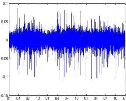
Figure 3.4The residuals after the ARX model, unit in percentage of the observed data.

More detailed result will be presented in the Result in section 4.

3.8 Simulation

When simulating the first day, the AR process of the model needs input from the 25 hours before. The previous year’s last 25 hours are used as input data and the sensitiveness of the initial values will be tested in section 4, Results. Otherwise the simulated data is used as input for the autoregressive parameters. In this section the method for simulating this model is going to be described.

3.8.1 Path of the simulation

The model is being simulated by one step prediction meaning, by calculating the model output one step at the time. The simulation will be a continuation of the first 25th_{observed data and therefor is the input of the autoregressive}

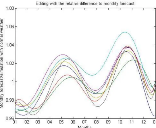
parameters. Certain deterministic parameters needs to be updated in each year, those who varies are days since the day of the week will be different, public holiday will also be different. In the price model the temperature input data are historical temperature data from the last 46 years. The output from the simulation will be 46 scenarios depending on the weather. The temperature used as input will be approximations in two ways, it will be distributed throughout the hours of the day based on a daily mean and approximated daily profile of temperature, will be written more of in part 3.6. For each step a noise is added and the time invariant variables are updated continuously as the next step is calculated.

3.9 Bootstrap of residuals, adding noise

After an ARX model is fitted to the electricity consumption data, the output of the ACF of the residuals do not contain any significant lags referring to correlation in

Forecasting Model of Electricity Demand in the Nordic Countries