Robust and model-independent cosmological constraints from distance measurements
Zhongxu Zhai∗ and Yun WangIPAC, California Institute of Technology, Mail Code 314-6, 1200 E. California Blvd., Pasadena, CA 91125∗
We present a systematic analysis of the cosmological constraints from the “Pantheon Sample” of 1048 Type Ia Supernovae (SNe Ia) in the redshift range 0.01<z<2.3 compiled by Scolnic et al. (2018). Applying the flux-averaging method for detecting unknown systematic effects, we find that the “Pantheon” sample has been well calibrated and the bias caused by unknown systematic errors has been minimized. We present the estimate of distances measured from SNe Ia and reconstruct the expansion history of the Universe. The results are in agreement with a simple cosmological constant model and reveals the possible improvements that future SN Ia observations from WFIRST and LSST can target.
We have derived distance priors using the Cosmic Microwave Background (CMB) data from the Planck 2018 final data release, and combine them with SNe Ia and baryon acoustic oscillation (BAO) data, to explore the impact from the systematic errors of SNe Ia on the combined cosmological parameter constraints. Using the combined data set of SNe Ia, BAO, and CMB distance priors, we measure the dark energy density function
X(z) =ρX(z)/ρX(0) as a free function (defined as a cubic spline of its values atz= 0.33,0.67,1.0), along with
the cosmological parameters (Ωk, Ωm, Ωb, H0). We find no deviation from a flat Universe dominated by a
cosmological constant (X(z) = 1), andH0= 68.4±0.9 km s−1Mpc−1, straddling the Planck team’s measurement
of H0= 67.4±0.5 km s−1Mpc−1, and Riess et al. (2018) measurement ofH0= 73.52±1.62 km s−1Mpc−1.
AddingH0= 73.52±1.62 km s−1Mpc−1as a prior to the combined data set leads to the time dependence of the
dark energy density atz∼0.33 at 68% confidence level. Not including the systematic errors on SNe Ia has a similar but larger effect on the dark energy density measurement.
I. INTRODUCTION
The accelerated expansion of the Universe has been one of the greatest mysteries in modern cosmology since it was first discovered through the observations of supernovae [1, 2]. The interpretation of this phenomena motivates the concept of dark energy, which dominates the total energy in the present-day observable Universe. As the mathematically simplest so-lution, the cosmological constant can well match the current observations. But there are arguments in the literature that the state-of-art observations imply deviations from the cosmolog-ical constant, e.g. [3–7] and references therein. Therefore it is necessary to perform a systematic and consistent analysis of the observational data so as to arrive at robust and model-independent constraints on the properties of dark energy [8].
In this paper, we investigate the possible unknown system-atic uncertainties in the latest observational data from Type Ia supernovae (SNe Ia), the “Pantheon Sample” which consists of 1048 SNe Ia in the redshift range 0.01<z<2.3 [9]. On the other hand, the Planck team has released the final product of the cosmic microwave background (CMB) measurement from the Planck mission [10, 11], which improves the con-straints from the previous releases and favors a spatially-flat 6-parameterΛCDM cosmology. Additionally, galaxy cluster-ing measures the distance scales through the Baryon Acous-tic Oscillation (BAO) at various redshifts [12]. These mea-surements probe the Universe with different methodologies, therefore they have different systematic uncertainties, and a consistency check is necessary to ensure a robust constraint on dark energy [13]. On the other hand, the CMB observa-tions from the Planck mission indicate a measurement on the
∗zhai@ipac.caltech.edu
Hubble constantH0that is in tension with the local measure-ment from the distance ladder. Compared with the latest mea-surement using data from Gaia [14], this discrepancy is higher than 3.6σ. Whether this discrepancy implies the unknown sys-tematic error in either observations, or signifies novel physics beyond our current understanding of cosmology is important for the survey strategies in the next decades. In this paper, we also investigate the impact of imposing this latestH0distance ladder measurement as a prior on the dark energy constraint.
Our paper is organized as follows. In Section 2, we out-line the models of dark energy we use in the analysis. Section 3 presents our analysis of the Pantheon SNe Ia data, includ-ing the search for unknown systematic errors usinclud-ing the flux-averaging method, and the measurement of the cosmic expan-sion history. In Section 4, we show results from combinations of different observational datasets. We discuss and conclude in Section 5.
II. METHODOLOGY
We focus on the the distance measurements of the Universe in this paper, i.e. the geometrical expansion history of the Universe, thus we do not consider the contribution from the growth rate of the cosmic large scale structure. The model is based on a FRW metric, under which the comoving distance to an object at redshiftzis given by
r(z) = c H0| Ωk|−1/2sinn[|Ωk|1/2Γ(z)], (1) Γ(z) = Z z 0 dz0 E(z0), E(z) =H(z)/H0, (2) where c is the speed of light, H0 = 100hkm s−1Mpc−1 with h the dimensionless Hubble constant, sinn(x) =
sin(x),x,and sinh(x) forΩk<0,Ωk= 0,andΩk>0, respec-tively. The Hubble parameterH(z) is given by
H(z)2=H02[Ωm(1+z)3+Ωr(1+z)4+Ωk(1+z)2+ΩΛX(z)], (3) with constraintΩm+Ωr+Ωk+ΩΛ= 1. The function X(z)≡ ρX(z)/ρX(0) describes the evolution of dark energy density with time. The radiation termΩr=Ωm/(1+zeq)Ωm can be omitted in the late time studies of dark energy andzeq is the redshift of matter-radiation equality. Ωkdenotes the con-tribution from spatial curvature.
The cosmological constant corresponds toρX =const. For comparison with this simplistic model, we also consider pa-rameterizations of the equation of state of dark energyw(z)
ρX(z) ρX(0)
= (1+z)3(1+w(z)). (4)
The first model is to assume w(z) =const (hereafter wCDM model). In this case, theΛCDM model is a special class when w=−1. The second model is linear parameterization of the cosmic scale factora= 1/(1+z) [15, 16] (hereafterw0waCDM model)
w(z) =w0+(1−a)wa, (5) wherew0andwaare free parameters to be determined by ob-servational data. Note thatwCDM andΛCDM model are just special classes whenw0andwaare fixed with particular val-ues.
Finally, we consider a model-independent parameterization ofX(z) =ρX(z)/ρX(0), whereX(z) is a free function of redshift given by the cubic spline of its values atz= 1/3,2/3 and 1.0 and assume thatX(z>1) =X(z= 1). This model has been investigated by [8, 17].
III. ANALYSIS OF TYPE IA SUPERNOVAE DATA
A. Flux averaging
The published SNe data are usually analyzed in terms of the distance modulus µ0≡m−M= 5 log d L(z) Mpc +25, (6)
wheremandM are apparent and absolute magnitude of each supernova respectively, and the luminosity distance is given bydL(z) = (1+z)r(z).
The SNe dateset considered in this paper is the Pantheon sample. This compilation contains the full set of specc-troscopically confirmed Pan-STARRS1 (PS1) SNe Ia and in combination with spectroscopically confirmed SNe Ia from CfA1-4, CSP, PS1, SDSS, SNLS andHubble Space Telescope (HST)SN surveys [9]. The (cross-)calibration of these SN samples can reduce the systematics substantially and the de-tails be found in [9, 18, 19] and references therein.
Due to the degeneracy betweenH0and the absolute magni-tude, the Pantheon sample reports the corrected magnitude for
each SN. In the cosmological analysis, this can be marginal-ized by the method presented in [20]. In addition, we use the unbinned, full SN data set instead of the binned version to be in line with general community reproducibility [9]
In the cosmological analysis of SNe data, one of the main systematics is the weak gravitational lensing induced by galaxies because of the inhomogeneous distribution of matter in the Universe [13]. One way to remove or reduce gravitational-lensing bias is through flux averaging [13]. Be-cause of flux conservation, the average magnification of a suf-ficient number of SNe at the same redshift is unity. And thus this process can recover the unlensed brightness of the SNe and yield cosmological parameter estimations without bias from weak gravitational lensing [21]. An important additional benefit of flux-averaging is that it effectively reduces a global systematic bias (over the entire redshift range) into a local bias (within each redshift bin) with a much smaller ampli-tude. Thus flux-averaged SN Ia data should be significantly less affected by unknown systematic biases (such as weak lensing or imperfect K-correction) than SNe Ia data without flux-averaging [22].
We explore the cosmological parameter constraints through theχ2 statistics combined with Markov Chain Monte Carlo (MCMC). Our flux-averaging method follows [8] and the steps are summarized below:
1. Convert the distance modulus of SNe Ia into “fluxes”:
F(zl) = 10(µ data 0 (zl)−25)/2.5 = ddata L (zl) Mpc −2 . (7)
2. Remove the redshift dependence of these “fluxes” to ob-tain their “absolute luminosities”L(zl) by assuming a set of cosmological parameterss,
L(zl)≡F(zl)dL2(zl|s). (8) 3. Flux-average the “absolute luminosities” L(zl) in each redshift binito obtainL¯iand mean redshift
¯ Li= 1 Ni Ni X i=1 Li l(z (i) l ), z¯i= 1 Ni Ni X l=1 z(li), (9)
whereNiis the number of SNe ini−th redshift bin. 4. PlaceL¯iat the mean redshiftz¯
ito get the binned flux ¯
F(z¯i) =L¯i/d2
L(z¯i|s), (10) and the flux-averaged distance modulus
¯
µdata(z¯i) =
−2.5 log10F¯(z¯i)+25. (11) 5. The new covariance matrix of µ¯(z¯i) and µ¯(z¯j) can be computed by Cov[µ¯(z¯i),µ¯(z¯j)] = 1 NiNjL¯iL¯j· (12) Ni X l=1 Nj X m=1 L(z(li))L(z(mj))h∆µdata 0 (z (i) l )∆µ data 0 (z(mj))i, (13)
whereh∆µdata 0 (z (i) l )∆µ data 0 (z (j)
m)iis the covariance between the corresponding SN Ia pairs from the measured distance moduli.
6. The finalχ2of this flux-averaged dataµ¯(¯z
i) can be com-puted as
χ2=X i j
∆¯µ(¯zi)Cov−1[µ¯(z¯i),µ¯(z¯j)]∆¯µ(¯zj), (14)
where∆¯µ(¯zi)≡µ¯(¯zi)−µp(¯zi|s), andµp(¯zi|s) can be computed for a given cosmological model.
In order to compare the effect of flux-averaging of SNe, we also perform a “magnitude-averaging” analysis. In this framework, the “magnitude-averaged” distance moduli in the i−th redshift bin is just the mean of all the SNe in this redshift bin. The results of flux-averaging and magnitude-averaging are compared with the unbinned full Pantheon sample, and any systematic bias can be revealed by the offset in the cosmo-logical parameter constraints. In our calculation, we adopt the same redshift binning scheme as the binned Pantheon sample and explore effect of binning width. We apply these methods to non-flatΛCDM model and flatwCDM model, which has parameter set (Ωm,ΩΛ) and (Ωm,w) respectively. Our results are shown in Figure 1 and Figure 2. In order to explore the im-pact from systematic error of supernovae data, we also show results with and without adding in the systematic covariance matrix in the analysis. The result is consistent with the analy-sis in [9]: the systematic uncertainties degrade the constraints on the cosmological parameters and also induce a shift in the best-fit values. This is true for both models in the figures and the shift can be attributed to the systematics in the low red-shift data [9]. A detailed discussion of the effects and origins of systematic uncertainties can be found in the Pantheon paper [9] as well.
The SNe sample with flux-averaging shows very consistent constraints with the unbinned full sample as we can see from the figures and this is true for both models. The best-fit values have a offset much smaller than 1σespecially when the sys-tematic uncertainties are taken into account. This result also shows that the original Pantheon sample has been very well cleaned and the bias induced by unknown systematic effects has been minimized. Since the weak lensing effect cannot be removed, this indicates that weak lensing effects are small for the Pantheon sample. On the other hand, the SNe sam-ple with magnitude-averaging shows obvious offset in the pa-rameter constraints. It is more significant when we increase the width of the redshift bin which results a >1σ tension for both ΛCDM and wCDM models when only the statisti-cal error is applied. The addition of systematic uncertainties can alleviate the tension for magnitude-averaging at some ex-tent but the difference is still quite noticeable. The results of flux-averaging and magnitude-averaging are quite different because different quantities are averaged in a given redshift bin. The quantity averaged in flux-averaging is an “absolute luminosity” which doesn’t have redshift dependence and is thus independent from redshift binning. However, this is not true for magnitude-averaging and may induce redshift-binning dependent bias in the cosmological constraints. The consis-tency between the flux-averaing method and the full unbinned result shows that flux-averaging can give robust cosmological
constraints, and the flux-averaged SN data can also serve as an alternative to compress the full SNe data for cosmological analysis [23].
B. Model-independent distance measurements from SNe Ia
In order to obtain an intuitive understanding of the SNe Ia data, [17] propose a scaled distance measure
rp(z) = rz cH−1
0 z
(1+z)0.41, (15)
wherer(z) is the comoving distance given by Eq. (1). This scaled distance can be measured from the SNe data, and the value at arbitrary redshift is given by cubic-spline interpola-tion, without explicitly assuming a cosmological model. The power 0.41 is chosen to make this distance as flat as pos-sible over the redshift range of interest [17]. This scaled distance also provides a way to examine the difference of flux-averaging and magnitude-averaging methods. It is worth pointing out that the Pantheon sample reports corrected dis-tance modulus instead of a raw measurements. It won’t affect the cosmological constraints due to the marginalization algo-rithm. However it should be accounted for in the distance measurements. In our calculation, we assume it can be cor-rected by a constant offset between the reported distance mod-ulus and the model prediction. We find this offset by a sim-ple linear fit with a best-fit cosmology constrained by the full unbinned dataset. This model is also used to obtain the flux-averaged and magnitude-flux-averaged SNe data. With 40 redshift bins, our measurements ofrpare shown in Figure 3. For com-parison, the theoretical predictions from the constrained non-flatΛCDM and flatwCDM are also shown.
Compared with the model prediction, the flux-averaged distance measurements have smaller dispersion than the magnitude-averaged data. It is consistent with the fact that flux-averaging can return betterχ2 in the data-model fitting [13]. In addition, the figure shows that the data points have deviations from theΛCDM andwCDM cosmology at redshift z∼0.1, implying that future observations at this redshift range will be very informative and provide useful cosmological con-straints.
C. Cosmic expansion history from SNe Ia
The SNe data can constrain the cosmic expansion history H(z) in principle. However the optimal way of doing this is still challenging in practice [24]. With the distance mod-ulus measured from SNe, [22] present a optimal method to measureH(z) in uncorrelated redshift bins. Since the latest Pantheon sample is much larger than the datasets analyzed in those works, it is worth revisiting this problem and investi-gate the implications. Note that the method in [22] assumes that the SNe measurements are uncorrelated. This condition is satisfied when we only consider the statistical uncertainty. Taking into account the systematic uncertainties may degrade the robustness of this analysis due to the correlated nature of
0.15 0.30 0.45
Ω
m 0.6 0.8 1.0 1.2Ω
Λ Unbinned SNe Magnitude-averaged SNe Flux-averaged SNe 0.15 0.30 0.45Ω
m 0.6 0.8 1.0 1.2Ω
Λ Unbinned SNe Magnitude-averaged SNe Flux-averaged SNe 0.15 0.30 0.45Ω
m 0.6 0.8 1.0 1.2Ω
Λ Unbinned SNe Magnitude-averaged SNe Flux-averaged SNe 0.15 0.30 0.45Ω
m 0.6 0.8 1.0 1.2Ω
Λ Unbinned SNe Magnitude-averaged SNe Flux-averaged SNeFIG. 1. Parameter constraints for a non-flatΛCDM cosmology with full unbinned Pantheon sample (blue), flux-averaged sample (red) and magnitude-averaged sample (green). The left and right panels assume analysis without and with systematic uncertainties respectively. The top row adopts the same redshift binning scheme as the Pantheon paper provides which has 40 bins, the bottom row adopt the binning scheme with a downsampling factor of 2, resulting 20 bins.
the systematic uncertainties. In our calculation, we ignore the off-diagonal elements in the systematic covariance matrix and it may not have significant effect since the systematic tainty is in general much smaller than the statistical uncer-tainty in the Pantheon sample.
Our method to measure the cosmic expansion history is de-scribed in detail by [22] and we summarize below. We first convert the distance modulusµ0of the SNe to comoving
dis-tance through r(z) 1Mpc= 1 2997.9(1+z)10 µ0/5−5. (16)
And for individual SN, its comoving distance is added by a noise term
0.15 0.30 0.45
Ω
m −2. 0 −1. 6 −1. 2 −0. 8w
Unbinned SNe Magnitude-averaged SNe Flux-averaged SNe 0.15 0.30 0.45Ω
m −2. 0 −1. 6 −1. 2 −0. 8w
Unbinned SNe Magnitude-averaged SNe Flux-averaged SNe 0.15 0.30 0.45Ω
m −2. 0 −1. 6 −1. 2 −0. 8w
Unbinned SNe Magnitude-averaged SNe Flux-averaged SNe 0.15 0.30 0.45Ω
m −2. 0 −1. 6 −1. 2 −0. 8w
Unbinned SNe Magnitude-averaged SNe Flux-averaged SNeFIG. 2. The same as Figure 1 but for flatwCDM cosmology.
where the noiseniis drawn from a Gaussian distribution with zero mean, and dispersionσicalculated from the error propa-gation ofµ0,i.
The next step is to sort the SNe by increasing redshift and define the quantities
xi≡ ri+1−ri zi+1−zi = Rzi+1 zi dz0 H(z0)+ni+1−ni zi+1−zi (18) = ¯fi+ ni+1−ni ∆zi , (19)
where∆zi=zi+1−ziand ¯fiis the average of 1/H(z) over the
redshift range (zi,zi+1). We note that in the Pantheon sample, there are several SN Ia pairs that have the same redshift, which prevents the redshift sorting. As a conservative choice, we just select the SN with larger uncertainty. In the above model,xi gives an unbiased estimate of the average of 1/H(z) in the redshift bin, sincehxii= ¯fi. Thus the inverse can be used to probe the cosmic expansion history. The covariance matrix of xican be calculated as Ni,i−1=− σ 2 i ∆zi−1∆zi, Ni,i= σ2 i+σi2+1 ∆z2 i , (20) Ni,i+1=− σi2+1 ∆zi∆zi+1, (21)
0.01 0.1 1.0 2.0 z 0.85 0.90 0.95 1.00 1.05 1.10 1.15 rp ( z )
1048 SNe Ia from the Pantheon sample
Best-fitoΛCDM 1σuncertainty ofoΛCDM 1σuncertainty ofwCDM Magnitude-averged SNe Flux-averaged SNe
FIG. 3. Distance measurements from the SNe Ia dataset. The model prediction from the best-fitoΛCDM model is shown as the blue solid line. The shaded areas represent the 1σuncertainty from the MCMC chains.
with all other entries to be zero. This new data vectorxiand the covariance matrix express the cosmic expansion history in very fine redshift bins, but with significant noise contribution. Therefore the next step is to average these noisy measure-ments into minimum-variance measuremeasure-ments in wider redshift bins. We usexbto denote the subset ofx
iin theb-th redshift bin and Nb the corresponding covariance matrix, then their weighted averageybcan be written as
yb=wb·xb (22) with some weight vectorwb. This weight vector can be ob-tained by minimizing the variance
∆y2b≡ hy2bi−hybi2=wbtNbwb, (23) subject to the constraint that the weights add up to unity, where the superscriptt refers to matrix transpose. The so-lution to this problem by the use of the Lagrange multiplier method is
wb= N
−1 e
etN−1e, (24)
whereeis the unit vector with all elements equal to 1. This weight vector is also calledwindow f unction, since it shows the contribution to the measurementsyb from different red-shifts. The uncertainty of measurementyb can be calculated by substituting the weight vector to Eq (23)
∆yb= (etN−1e)−1/2. (25) Figure 4 shows our measurements of the expansion his-tory through this method for two different redshift binning schemes, as well as the prediction from the best-fit model and
95 % uncertainties. While the reconstruction result is in agree-ment with theΛCDM model, the high redshift bin has appar-ent deviation. This is due to the limited number of SNe in this redshift bin, and can be improved when multiple bins are combined as shown by the blue square at high redshift. The middle and bottom panels show the window functions Eq (24) of the reconstructions. Due to noisy nature of the SNe dataset, the window function only shows weak characteristics as pre-sented in [22]: an upside-down parabola vanishing at the bin end points and maximize near the center of the bin. Clearly, the measurement ofH(z) from SNe Ia can be significantly im-proved with thez<0.8 SNe Ia from LSST[25], and thez>1 SNe Ia from WFIRST [26].
1.0 1.2 1.4 1.6 1.8 2.0 2.2 H ( z ) /H 0
1025 SNe Ia from the Pantheon sample ΛCDM(Ωm= 0.323,ΩΛ= 0.743) Nbin=10 Nbin=5 0.000 0.025 0.050 0.075 0.100 w eig ht Nbin=10 0.0 0.2 0.4 0.6 0.8 1.0 1.2
z
0.000 0.025 0.050 0.075 0.100 w eig ht Nbin=5FIG. 4. The top panel shows the cosmic expansion history expressed in terms of dimensionless Hubble parameter, using the reconstruction method for SNe data. The solid line and grey area is the best-fit
ΛCDM model and 95 % uncertainty. The measurements from data are shown with two redshift binning schemes which have 10 and 5 redshift bins respectively. The middle and bottom panels present the corresponding window functions in the reconstruction.
IV. COMBINATION WITH OTHER DATASETS
In order to improve the cosmological constraints, it is use-ful to include measurements from other probes. In this paper, we employ the data from CMB, BAO andH0 to better
un-derstand their impacts on the estimation of the cosmological parameters.
A. CMB data
We use the CMB data from the latest and final Planck data release [11]. Its contribution in the likelihood analysis is ex-pressed in terms of the comex-pressed form with CMB shift pa-rameters [27, 28]:
R≡ q
ΩmH02r(z∗)/c, (26)
la≡πr(z∗)/rs(z∗), (27) wherers(z) is the comoving sound horizon at redshiftz, and z∗is the redshift to the photon-decoupling surface. These two CMB shift parameters together withωb=Ωbh2 and spectral index of the primordial power spectrumns can give an effi-cient summary of CMB data for the dark energy constraints.
The comoving sound horizon is given by
rs(z) = Z t 0 csdt0 a = c H0 Z ∞ z dz0 cs E(z0) = c H0 Z a 0 da0 p 3(1+R¯ba0)a04E2(z0) . (28)
The radiation term in the expression of E(z) for the CMB data analysis shouldn’t be ignored. It can be determined by the matter-radiation equality relation Ωr =Ωm/(1+zeq), and
zeq = 2.5×10⁴ωm(TCMB/2.7K)−4, where ωm =Ωmh2. The sound speed iscs= 1/
p
3(1+R¯ba), withR¯ba= 3ρb/(4ρr), and ¯
Rb= 31500wb(TCMB/2.7K)−4. We assume the CMB tempera-tureTCMB= 2.7255K.
The redshiftz∗can be calculated by the fitting formula [29]: z∗= 1048[1+0.00124ωb−0.738][1+g1ωgm2], (29) where g1= 0.0783ω−0.238 b 1+39.5ω0.763 b , g2= 0.560 1+21.1ω1.81 b . (30)
The Planck data we use for the analysis include temperature and polarization data, as well as CMB lensing. In particular, we use the base_plikHM_TTTEEE_lowl_lowE_lensing
in the base MCMC chain, and
base_omegak_plikHM_TTTEEE_lowl_lowE_lensing in the base_omegak MCMC chain to get two versions of the compressed Planck CMB data for a spatailly-flat and non-flat model respectively. The final result is expressed in terms of a data vectorv= (R,la, ωb,ns)tand their covariance matrix.
For a flat universe, this data vector is
v= 1.74963 301.80845 0.02237 0.96484 (31)
and the covariance matrix is Cv= 10−8× 1598.9554 17112.007 −36.311179 −1122.4683 17112.007 811208.45 −494.79813 −11925.120 −36.311179 −494.79813 2.1242182 23.779841 −1122.4683 −11925.120 23.779841 1725.4040 .
For a non-flat universe, the corresponding data vector and co-variance matrix are
v= 1.74451 301.76918 0.022483 0.96881 (32) Cv= 10−8× 2556.7782 23212.222 −57.345815 −1847.3003 23212.222 830122.02 −628.56261 −17499.134 −57.345815 −628.56261 2.5300094 39.666623 −1847.3003 −17499.134 39.666623 2225.2344 .
Note that the non-flat compression of the Planck CMB data has larger variance than the flat counterpart due to the added degree of freedom fromΩk. This compression of CMB data forms the so-called distance priors [27]. The compression of CMB data presented here is not exclusive. Examples from other MCMC chains of the Planck 2018 release can be found in the literature, e.g. [30]. For completeness, we include the spectral indexnsin the distance prior calculation as well. In the study of the purely geometrical expansion of the universe as in this paper, this data point can be marginalized over [8].
B. BAO data
The BAO data represent the absolute distance measure-ments in the Universe. From the measuremeasure-ments of correlation function or power spectrum of large scale structure, we can use the BAO signal to estimate the distance scales at differ-ent redshifts. In practice, the BAO data are analyzed based on a fiducial cosmology and the sound horizon at drag epoch. For instance, in an anisotropic analysis, we can measure the comoving angular diameter distanceDM(z) and the Hubble parameterH(z) [31]
DM(z)/rd=α⊥DM,fid/rd,fid, (33)
DH(z)/rd=αkDH,fid/rd,fid, (34) whereDH(z) =c/H(z) andrdis the sound horizon at the drag epochzd, the subscript “fid” represents the quantity in the as-sumed fiducial cosmology. We calculate the redshift of the drag epoch as [32] zd= 1291ω0.251 m 1+0.659ω0.828 m [1+b1ωbb2], (35) where b1= 0.313ωm−0.419[1+0.607ω 0.674 m ], (36) b2= 0.238ω0m.223. (37)
In this paper, we use the BAO measurements atz= 0.106 from 6dFGS [33], z= 0.15 from SDSS-Main Galaxy Sam-ple (MGS, [34]), the final DR12 BOSS measurements at red-shiftz= 0.38,0.51,0.61 [35],z= 1.52 from the eBOSS QSO sample [36], and the Lyα forest measurements from auto-correlation [37] and cross auto-correlation [38] from BOSS survey.
C. The Hubble constant
The Hubble constant measures the current expansion rate of the Universe. The determination of its value and uncer-tainty has attracted significant attention for decades. How-ever, its latest measurements from the distance ladder method and CMB observation of the early Universe reveal a contro-versial tension [39]. With the data from Gaia parallaxes, [14] report a measurement ofH0= 73.52±1.62 km s−1Mpc−1, in agreement with earlier measurement from Hubble space tele-scopeH0= 73.48±1.66 km s−1Mpc−1 [40]. However, these measurements are in significant tension with the latest mea-surement by the Planck team using their CMB data [11], H0= 67.27±0.602 km s−1Mpc−1. This 3.6σdiscrepancy has motivated a large number of papers that investigate it from different aspects, including the possible systematic error in the Planck data [41], the sample variance of the local mea-surement ofH0[42], the statistical impact from the likelihood assumption [43], and possible implications of different cos-mological models [44–46].
In this paper, we apply the latest measurement from [14], and investigate its impact on the dark energy and cosmologi-cal parameter constraints. The combination with other probes including SNe and CMB can also provide hint for the study the of dark energy property, and examine possible systematic errors. We constrainH0using SNe Ia, BAO, and Planck CMB distance priors, to compare with other measurements.
D. Results
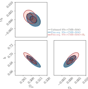
Figure 5 and 6 present the constraint on the parameters for non-flatΛCDM andwCDM model, the results are also sum-marized in Table I and II. Our results in Section III A show that the flux-averaged SN Ia data is in consistent with the full sample. We further investigate this effect by combining the SNe with other cosmological probes. When CMB and BAO data are used, we find that the constraints on the parameters are also identical and the resultant contours in the two figures are indeed indistinguishable. Thus we only report the results with flux-averaging of SNe in the remainder of this paper.
We also compare the effect of the systematic uncertainties from SNe on the cosmological constraints. The results in Ta-ble I and II show that ignoring the systematic errors in the SNe can degrade the cosmological constraints and shift the best-fit values. But the amount of change depends on cosmological models, i.e. flexibility of the model under consideration. For the simplestΛCDM model, the constraints onΩmandhcan degrade by 5% when the systematic errors of SNe is taken into account. However, the change in the parameters ofwCDM is
−0. 005 0.000 0.005 0.010 Ωk Unbinned SNe+CMB+BAO Flux-avg. SNe+CMB+BAO Flux-avg. SNe+CMB+BAO+H0 0.285 0.300 0.315 0.330 Ωm 0.66 0.68 0.70 0.72 h −0.005 0.000 0.005 0.010 Ωk
FIG. 5. Parameter constraints for the non-flatΛCDM model. For comparison, the result with unbinned SNe data in combination with CMB+BAO is also shown. Due to the consistency between the flux-averaged SNe sample and the full unbinned sample, the per-formance of unbinned SNe+CMB+BAO is nearly identical with the flux-averaged version, so the resulting contours are indistinguish-able. −1. 1 −1.0 −0. 9 −0. 8 w Unbinned SNe+CMB+BAO Flux-avg. SNe+CMB+BAO Flux-avg. SNe+CMB+BAO+H0 −0. 005 0.000 0.005 0.010 Ωk 0.66 0.68 0.70 0.72 h −1. 1 −1. 0 −0. 9 −0. 8 w
FIG. 6. Cosmological constraint for non-flatwCDM model, only parameter subset (Ωk,w,h) is shown.
Data sample Ωm Ωk h
SNe (stats)+CMB+BAO 0.3006±0.0059 0.0003±0.0019 0.6849±0.0063 SNe (stats)+CMB+BAO+H0 0.2951±0.0055 0.0017±0.0018 0.6916±0.0060
SNe+CMB+BAO 0.3041±0.0062 0.0001±0.0019 0.6818±0.0065
SNe+CMB+BAO+H0 0.2978±0.0058 0.0017±0.0018 0.6894±0.0062
TABLE I. Cosmological constraints for the non-flatΛCDM model. The SNe data are flux-averaged, “stats” in the parenthesis refers to statistical error only for SNe data.
Data sample Ωm Ωk w h
SNe (stats)+CMB+BAO 0.2982±0.0060 −0.0012±0.0020 −1.0494±0.0288 0.6891±0.0069
SNe (stats)+CMB+BAO+H0 0.2928±0.0056 −0.0002±0.0020 −1.0595±0.0284 0.6962±0.0064
SNe+CMB+BAO 0.3035±0.0077 −0.0001±0.0022 −1.0075±0.0397 0.6828±0.0086
SNe+CMB+BAO+H0 0.2942±0.0068 0.0004±0.0021 −1.0413±0.0382 0.6944±0.0078
TABLE II. Cosmological constraints for the non-flatwCDM model. The SNe data are flux-averaged. The value ofw=−1.0 corresponds to the
ΛCDM model. −0. 8 0.0 0.8 wa SNe (stats)+CMB+BAO SNe (stats)+CMB+BAO+H0 SNe+CMB+BAO SNe+CMB+BAO+H0 −1. 2 −1. 0 −0. 8 w0 0.66 0.68 0.70 0.72 h −0. 8 0.0 0.8 wa
FIG. 7. Constraints on parameters (w0,wa,h) for thew0wa
cosmol-ogy. SNe data are flux-averaged and the impact of systematic un-certainties is isolated. The dashed lines correspond tow0=−1.0 and
wa= 0.0.
larger. The typical change of the parameter uncertainties is higher than 20%. The largest change is the equation of state parameterwwhich can be affected by the SNe systematic er-ror with an amount of 35∼40%. It is due to the fact that SNe probe the late time expansion of the universe which is dom-inated by dark energy. Therefore it approves the necessity of the correct modeling of the systematic errors in the super-novae observations. On the other hand, the constraint on the spatial curvatureΩkis barely affected by the systematic error
of SNe, since most of the contribution is from CMB.
Figure 5 and 6 also present the effect of H0 measure-ment on the cosmological constraints. For instance, in the ΛCDM model, H0 = 68.18±0.65 km s−1Mpc−1 from the SNe+CMB+BAO constraints, implying a∼3σtension with the local measurement ofH0from the distance ladder method. Combining all the probes withH0measurement, the result is shown as the pink contours in the figures. It is obvious that the addition ofH0can shift the constraints towards the related degenerate direction. And the overall shift of the constraints is at 1σlevel. For the equation of state of dark energy, adding theH0measurement can push the constraint to the more neg-ative direction, implying a phantom behavior of dark energy [47–49]. Thus understanding thisH0 tension is important in the exploration of dark energy properties.
Figure 7 and Table III shows the constraint on the w0wa cosmology. The effects from SNe systematic error and H0 are both isolated in the figure. Due to the flexibility of this model, the difference between data combinations is obvious and also enhanced compared with previous simpler models. For the data combination SNe+CMB+BAO, the resulting con-straints onw0andwaare consistent with a cosmological con-stant model. However, when theH0 measurement is added, the current equation of state of dark energyw0favors a phan-tom value, same as the wCDM model. Moreover, it also slightly increaseswa, which changes the evolution ofw(z) in the past. The constraints without SNe systematic uncertainties are shown as the dashed contours. The results show that ig-noring this systematics have similar impact on the constraint ofw0asH0has, thus implying a “degeneracy” between theH0 measurement and SNe systematic errors. The constraint onwa is also affected by the SNe systematic error and the change of constraint is larger than that induced byH0. Since the sys-tematic errors of SNe have many components, for instance the Pantheon sample has 85 separate systematic uncertainties [9], understanding the correlation between the systemtaic er-ror and the effect ofH0on the cosmological parameter con-straint is non-trivial. But it will be useful for the study of dark
Data sample Ωm Ωk w0 wa h
SNe (stats)+CMB+BAO 0.2968±0.0062 0.0017±0.0036 −1.1315±0.0736 0.4444±0.3655 0.6905±0.0071
SNe (stats)+CMB+BAO+H0 0.2914±0.0058 0.0033±0.0038 −1.1540±0.0742 0.5185±0.3660 0.6979±0.0068
SNe+CMB+BAO 0.3039±0.0079 −0.0007±0.0034 −0.9863±0.0989 −0.1082±0.4815 0.6823±0.0088
SNe+CMB+BAO+H0 0.2940±0.0068 0.0008±0.0036 −1.0542±0.0971 0.0672±0.4853 0.6944±0.0080
TABLE III. Cosmological constraints for the non-flatw0waCDM model. The SNe data are flux-averaged in the analysis.
Data sample Ωm X(0.33) X(0.67) X(1.0) h
SNe (stats)+CMB+BAO 0.2936±0.0061 0.9374±0.0299 1.0286±0.0600 0.7667±0.3272 0.6940±0.007 SNe (stats)+CMB+BAO+H0 0.2886±0.0057 0.9283±0.0284 1.0242±0.0588 0.7150±0.3285 0.7008±0.0067
SNe+CMB+BAO 0.3024±0.0079 0.9915±0.0422 1.0473±0.0861 0.8372±0.3645 0.6841±0.0090 SNe+CMB+BAO+H0 0.2923±0.0068 0.9554±0.0402 1.0157±0.0801 0.7357±0.3412 0.6964±0.0078
TABLE IV. Cosmological constraints for the model-independent parameterization ofX(z). The SNe data are flux averaged in the analysis.
energy.
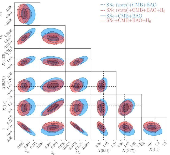
We present the constraints on the model-independent parametrization ofX(z) in Figure 8 and Table IV. This model is flexible to model the late evolution of the universe, and we show the constraints for the full parameter set in the figure. Compared with thew0wa cosmology, the impacts from SNe systematic error and H0 measurements are similar. In Fig-ure 9, we present the evolution of the dark energy density function X(z) =ρX(z)/ρX(0). The black dashed-line corre-sponds to cosmological constant, which is well within 1σ con-straint from SNe+CMB+BAO dataset, implying thatΛCDM model is able to describe the current observations. The result also shows the effect fromH0 measurement which indicates a 1−2σdeviation from cosmological constant in the redshift range 0<z<0.33, and this data point also forces the evolu-tion ofX(z) more dynamical. This tension-motivated result is also previously investigated in [3] with more details.
V. DISCUSSION AND CONCLUSION
We have performed a systematic analysis of the latest SNe Ia sample, namely the “Pantheon” sample. We apply the flux-averaging method to this dataset to detect and minimize un-known systematic effects, and compare the cosmological con-straints with the original unbinned data. The results show that the original SNe data give constraints on non-flatΛCDM and flatwCDM cosmology that are consistent with the flux-averaged data. This indicates that the “Pantheon” sample has been cleaned and the systematic error from unknown system-atic errors has been minimized, and that weak lensing effects are small for this sample. In addition, it supports the use of flux-averaged SN Ia data as an alternative to compress the SNe data for the cosmological usage. We also use these SNe data to measure the distance scale in Eq (15) and compare with the best-fitΛCDM model. The result shows that future super-nova observation at redshift z∼0.1 will be informative and can provide more constraining power on cosmological param-eters. As another application of the “Pantheon” SNe sample, we use the method from [22] to measure the cosmic
expan-sion historyH(z) from flux-averaged SN Ia data. The result presented in Fig 4 shows consistency with the simpleΛCDM cosmology, an interesting cross-check using a method insen-sitive to certain systematic uncertainties in the SNe dataset [22]. This also highlights the progress that can be made with the future SN Ia from LSST atz<0.8 and WFIRST atz>1.
In order to improve the cosmological constraints, we com-bine this SN Ia sample with the latest CMB and BAO data. In particular, we use the CMB distance priors that we have de-rived from Planck 2018 final data release, and the BAO mea-surements distributed in a wide redshift range. We use these data combinations and investigate the constraints on the evolu-tion of dark energy. For flexible models likew0waand model-independent parametrization of dark energy density, we find that the deviation from a cosmological constant is not signifi-cant. The simplestΛCDM model can explain the current ob-servations with high significance. In addition, we explore the impacts from the systematic uncertainties of SNe and the local measurement ofH0on the cosmological constraints.
Using the combined SNe, BAO data, and Planck CMB distance priors, we find no deviation from a flat Universe dominated by a cosmological constant, and H0 = 68.4± 0.9 km s−1Mpc−1, straddling the Planck team’s measurement of H0 = 67.4±0.5 km s−1Mpc−1, and Riess et al. (2018) measurement of H0 = 73.52±1.62 km s−1Mpc−1. Adding
H0= 73.52±1.62 km s−1Mpc−1 as a prior to the combined data set leads to the time dependence of the dark energy den-sity atz∼0.33 at 68% confidence level (see Figure 9). Not including the systematic errors on SNe Ia has a similar but larger effect on the dark energy density measurement. These results may indicate possible correlations between the SNe Ia systematic errors andH0 measurements. Understanding the detailed correlations can be challenging due to the compli-cated nature of SNe Ia observations, but also useful, since the H0measurement built on distance ladders involves the obser-vation of supernovae.
Identifying and correcting the potential systematic effects in the cosmological observations is crucial in the study of dark energy [50]. As future survey plans will accumulate large amounts of data, systematic uncertainties can be the limiting
−0. 006 0.000 0.006 Ωk
SNe (stats)+CMB+BAO
SNe (stats)+CMB+BAO+H
0SNe+CMB+BAO
SNe+CMB+BAO+H
0 0.0425 0.0450 0.0475 0.0500 Ωb 0.90 1.05 1.20 X (0 . 33) 0.90 1.05 1.20 1.35 X (0 . 67)) 0.0 0.6 1.2 1.8 X (1 . 0) 0.2850.3000.3150.330 Ωm 0.66 0.68 0.70 0.72 h −0. 006 0.000 0.006 Ωk 0.04250.04500.04750.0500 Ωb 0.90 1.05 1.20 X(0.33) 0.90 1.05 1.20 1.35 X(0.67)) 0.0 0.6 1.2 1.8 X(1.0)FIG. 8. Cosmological constrains on the model-independent parameterization ofX(z). The dashed lines forX(z= 0.33,0.67,1.0) correspond to values of 1.0, i.e. cosmolgical constant. SNe data are flux-averaged in the analysis.
factor of cosmological analysis, and the correct modeling is important and necessary as we present in this paper. With more observations from ground or space [26, 51, 52], we can expect significant progress in our understanding of the universe in the coming decades.
ACKNOWLEDGMENTS
ZZ thanks Jeremy Tinker for helpful discussions and sug-gestions, and Savvas Nesseris for his comments. We ac-knowledge the use of the public softwares Matplotlib [53], NumPy [54], SciPy [55], and Emcee [56]. This work is sup-ported in part by NASA grant 15-WFIRST15-0008, Cosmol-ogy with the High Latitude Survey WFIRST Science Investi-gation Team (SIT).
[1] A. G. Riess, A. V. Filippenko, P. Challis, A. Clocchiatti, A. Diercks, P. M. Garnavich, R. L. Gilliland, C. J. Hogan,
astro-0.0
0.2
0.4
0.6
0.8
1.0
z
0.5
0.6
0.7
0.8
0.9
1.0
1.1
1.2
1.3
X
(
z
)
=
ρ
X
(
z
)
/ρ
X
(0)
Data used: SNe (Pantheon 2018); CMB (Planck 2018); H0(Riess 2018);
BAO (6dFGS + MGS + BOSS DR12 + eBOSS QSO + BOSS LyαF)
SNe (stats) + CMB + BAO
SNe (stats) + CMB + BAO + H0
SNe + CMB + BAO
SNe + CMB + BAO + H0
FIG. 9. The dark energy density functionX(z) =ρX(z)/ρX(0) for the model-independent parameterization. The area with shaded color or
enclosed by same line style correspond to 1σconfidence level. The horizontal black dashed line correspond toX(z) = 1, the black dots with errorbar are 1σconstraints from Flux-averaged SNe+CMB+BAO combination.
ph/9805201.
[2] S. Perlmutter, G. Aldering, G. Goldhaber, R. A. Knop, P. Nu-gent, P. G. Castro, S. Deustua, S. Fabbro, A. Goobar, D. E. Groom, et al., ApJ517, 565 (1999), astro-ph/9812133. [3] G.-B. Zhao, M. Raveri, L. Pogosian, Y. Wang, R. G. Crittenden,
W. J. Handley, W. J. Percival, F. Beutler, J. Brinkmann, C.-H. Chuang, et al., Nature Astronomy1, 627 (2017), 1701.08165. [4] J. Sola, A. Gomez-Valent, and J. de Cruz Perez, ApJ836, 43
(2017), 1602.02103.
[5] C.-G. Park and B. Ratra, ArXiv e-prints (2018), 1803.05522. [6] C.-G. Park and B. Ratra, ArXiv e-prints (2018), 1807.07421. [7] Y. Wang, L. Pogosian, G.-B. Zhao, and A. Zucca, ArXiv
e-prints (2018), 1807.03772.
[8] Y. Wang and M. Dai, Phys. Rev. D 94, 083521 (2016), 1509.02198.
[9] D. M. Scolnic, D. O. Jones, A. Rest, Y. C. Pan, R. Chornock, R. J. Foley, M. E. Huber, R. Kessler, G. Narayan, A. G. Riess, et al., ApJ859, 101 (2018), 1710.00845.
[10] Planck Collaboration, Y. Akrami, F. Arroja, M. Ashdown, J. Aumont, C. Baccigalupi, M. Ballardini, A. J. Banday, R. B. Barreiro, N. Bartolo, et al., ArXiv e-prints (2018), 1807.06205. [11] Planck Collaboration, N. Aghanim, Y. Akrami, M. Ashdown, J. Aumont, C. Baccigalupi, M. Ballardini, A. J. Banday, R. B. Barreiro, N. Bartolo, et al., ArXiv e-prints (2018), 1807.06209. [12] D. J. Eisenstein, I. Zehavi, D. W. Hogg, R. Scoccimarro, M. R. Blanton, R. C. Nichol, R. Scranton, H.-J. Seo, M. Tegmark,
Z. Zheng, et al., ApJ633, 560 (2005), astro-ph/0501171. [13] Y. Wang and P. Mukherjee, ApJ 606, 654 (2004),
astro-ph/0312192.
[14] A. G. Riess, S. Casertano, W. Yuan, L. Macri, B. Bucciarelli, M. G. Lattanzi, J. W. MacKenty, J. B. Bowers, W. Zheng, A. V. Filippenko, et al., ApJ861, 126 (2018), 1804.10655.
[15] M. Chevallier and D. Polarski, International Journal of Modern Physics D10, 213 (2001), gr-qc/0009008.
[16] E. V. Linder, Phys. Rev. Lett. 90, 091301 (2003), astro-ph/0208512.
[17] Y. Wang, Phys. Rev. D80, 123525 (2009), 0910.2492. [18] M. Betoule, J. Marriner, N. Regnault, J.-C. Cuillandre,
P. Astier, J. Guy, C. Balland, P. El Hage, D. Hardin, R. Kessler, et al., A&A552, A124 (2013), 1212.4864.
[19] D. Scolnic, S. Casertano, A. Riess, A. Rest, E. Schlafly, R. J. Foley, D. Finkbeiner, C. Tang, W. S. Burgett, K. C. Chambers, et al., ApJ815, 117 (2015), 1508.05361.
[20] A. Conley, J. Guy, M. Sullivan, N. Regnault, P. Astier, C. Bal-land, S. Basa, R. G. Carlberg, D. Fouchez, D. Hardin, et al., ApJS192, 1 (2011), 1104.1443.
[21] Y. Wang, ApJ536, 531 (2000), astro-ph/9907405.
[22] Y. Wang and M. Tegmark, Phys. Rev. D71, 103513 (2005), astro-ph/0501351.
[23] M. Betoule, R. Kessler, J. Guy, J. Mosher, D. Hardin, R. Biswas, P. Astier, P. El-Hage, M. Konig, S. Kuhlmann, et al., A&A568, A22 (2014), 1401.4064.
[24] M. Tegmark, Phys. Rev. D 66, 103507 (2002), astro-ph/0101354.
[25] LSST Science Collaboration, P. A. Abell, J. Allison, S. F. An-derson, J. R. Andrew, J. R. P. Angel, L. Armus, D. Arnett, S. J. Asztalos, T. S. Axelrod, et al., ArXiv e-prints (2009), 0912.0201.
[26] D. Spergel, N. Gehrels, C. Baltay, D. Bennett, J. Breckinridge, M. Donahue, A. Dressler, B. S. Gaudi, T. Greene, O. Guyon, et al., ArXiv e-prints (2015), 1503.03757.
[27] Y. Wang and P. Mukherjee, Phys. Rev. D76, 103533 (2007), astro-ph/0703780.
[28] Y. Wang and S. Wang, Phys. Rev. D 88, 043522 (2013), 1304.4514.
[29] W. Hu and N. Sugiyama, ApJ 471, 542 (1996), astro-ph/9510117.
[30] L. Chen, Q.-G. Huang, and K. Wang, ArXiv e-prints (2018), 1808.05724.
[31] É. Aubourg, S. Bailey, J. E. Bautista, F. Beutler, V. Bhardwaj, D. Bizyaev, M. Blanton, M. Blomqvist, A. S. Bolton, J. Bovy, et al., Phys. Rev. D92, 123516 (2015), 1411.1074.
[32] D. J. Eisenstein and W. Hu, ApJ 496, 605 (1998), astro-ph/9709112.
[33] F. Beutler, C. Blake, M. Colless, D. H. Jones, L. Staveley-Smith, L. Campbell, Q. Parker, W. Saunders, and F. Watson, MNRAS416, 3017 (2011), 1106.3366.
[34] A. J. Ross, L. Samushia, C. Howlett, W. J. Percival, A. Burden, and M. Manera, MNRAS449, 835 (2015), 1409.3242. [35] S. Alam, M. Ata, S. Bailey, F. Beutler, D. Bizyaev, J. A. Blazek,
A. S. Bolton, J. R. Brownstein, A. Burden, C.-H. Chuang, et al., ArXiv e-prints (2016), 1607.03155.
[36] M. Ata, F. Baumgarten, J. Bautista, F. Beutler, D. Bizyaev, M. R. Blanton, J. A. Blazek, A. S. Bolton, J. Brinkmann, J. R. Brownstein, et al., MNRAS473, 4773 (2018), 1705.06373. [37] T. Delubac, J. E. Bautista, N. G. Busca, J. Rich, D. Kirkby,
S. Bailey, A. Font-Ribera, A. Slosar, K.-G. Lee, M. M. Pieri, et al., A&A574, A59 (2015), 1404.1801.
[38] A. Font-Ribera, D. Kirkby, N. Busca, J. Miralda-Escudé, N. P. Ross, A. Slosar, J. Rich, É. Aubourg, S. Bailey, V. Bhardwaj, et al., Journal of Cosmology and Astroparticle Physics5, 027 (2014), 1311.1767.
[39] W. L. Freedman, Nature Astronomy 1, 0169 (2017), 1706.02739.
[40] A. G. Riess, S. Casertano, W. Yuan, L. Macri, J. Anderson, J. W. MacKenty, J. B. Bowers, K. I. Clubb, A. V. Filippenko, D. O. Jones, et al., ApJ855, 136 (2018), 1801.01120.
[41] G. E. Addison, Y. Huang, D. J. Watts, C. L. Bennett, M. Halpern, G. Hinshaw, and J. L. Weiland, ApJ 818, 132 (2016), 1511.00055.
[42] H.-Y. Wu and D. Huterer, MNRAS 471, 4946 (2017), 1706.09723.
[43] S. M. Feeney, D. J. Mortlock, and N. Dalmasso, ArXiv e-prints (2017), 1707.00007.
[44] E. Di Valentino, A. Melchiorri, and J. Silk, Physics Letters B
761, 242 (2016), 1606.00634.
[45] E. Di Valentino, A. Melchiorri, E. V. Linder, and J. Silk, Phys. Rev. D96, 023523 (2017), 1704.00762.
[46] Z. Zhai, M. Blanton, A. Slosar, and J. Tinker, ApJ850, 183 (2017), 1705.10031.
[47] R. R. Caldwell, Physics Letters B 545, 23 (2002), astro-ph/9908168.
[48] R. R. Caldwell, M. Kamionkowski, and N. N. Weinberg, Phys. Rev. Lett.91, 071301 (2003), astro-ph/0302506. [49] J. Ryan, S. Doshi, and B. Ratra, MNRAS480, 759 (2018),
1805.06408.
[50] S. Wang and Y. Wang, Phys. Rev. D 88, 043511 (2013), 1306.6423.
[51] DES Collaboration, T. M. C. Abbott, S. Allam, P. Andersen, C. Angus, J. Asorey, A. Avelino, S. Avila, B. A. Bassett, K. Bechtol, et al., ArXiv e-prints (2018), 1811.02374. [52] L. Amendola, S. Appleby, A. Avgoustidis, D. Bacon, T. Baker,
M. Baldi, N. Bartolo, A. Blanchard, C. Bonvin, S. Borgani, et al., Living Reviews in Relativity21, 2 (2018), 1606.00180. [53] J. D. Hunter, Computing in Science Engineering9, 90 (2007),
ISSN 1521-9615.
[54] S. van der Walt, S. C. Colbert, and G. Varoquaux, Computing in Science Engineering13, 22 (2011), ISSN 1521-9615. [55] E. Jones, T. Oliphant, P. Peterson, et al.,SciPy: Open source
scientific tools for Python(2001–), [Online; scipy.org], URL
http://www.scipy.org/.
[56] D. Foreman-Mackey, D. W. Hogg, D. Lang, and J. Goodman, PASP125, 306 (2013), 1202.3665.