The rule Extraction of Numerical Association Rule
Mining Using Hybrid Evolutionary Algorithm
Imam Tahyudin
Graduate School of Natural Science and Technology Electrical Engineering and Computer Science
Kanazawa University, Japan Email: [email protected]
Hidetaka Nambo
Graduate School of Natural Science and Technology Electrical Engineering and Computer Science
Kanazawa University, Japan Email: [email protected]
Abstract—The topic of Particle Swarm Optimization (PSO) has recently gained popularity. Researchers has used it to solve difficulties related to job scheduling, evaluation of stock markets and association rule mining optimization. However, the PSO method often encounters the problem of getting trapped in the local optimum. Some researchers proposed a solution to over come that problem using combination of PSO and Cauchy distribution because this performance proved to reach the optimal rules. In this paper, we focus to adopt the combination for solving association rule mining (ARM) optimization problem in numerical dataset. Therefore, the aim of this research is to extract the rule of numerical ARM optimization problem for certain multi-objective functions such as support, confidence, and amplitude. This method is called PARCD. It means that PSO for numerical association rule mining problem with Cauchy Distribu-tion. PARCD performed better results than other methods such as MOPAR, MODENAR, GAR, MOGAR and RPSOA.
I. INTRODUCTION
ARM is data mining method which is used to determine the relationship between variables in a dataset by using certain algorithms in to obtain useful patterns or rules [1]. The familiar algorithms of ARM are Apriori and FP growth algorithm [2]. Those are proper for categorical dataset such as sex and binary format. If the data is numerical dataset, such as age, weight, or length, it should be discretized to the interval form or group form [3]. However, this process has some drawbacks like lost important information and spent long time [4],[5].
Some authors have solved the numerical ARM problem by using the optimization method as well as genetic algorithm (GA), differential evolution, and PSO [6],[7]. Moreover, some authors have solved the problem by using mono-objective that use only support and confidence parameters whereas others used multi-objectives measurements, such as support, confidence, and amplitude. In addition, many studies have used the Pareto optimality for fitness computation; however, many other studies have not used Pareto optimality [2].
Recently, the PSO method was used for solving the ARM problem [5]. However, it has a weakness i.e., it gets trapped in local optimum and when the iteration becomes infinite, the particle velocity become 0 [8]. Therefore, it does not has the capability for searching optimal solution [8]. To overcome this weakness by combining PSO and Cauchy distribution. Li et. al., introduce this combination as a simple method that is robust for searching the optimal solution in a large database.
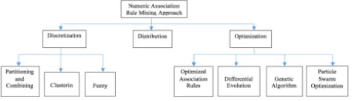
Fig. 1. Previous Work of Numerical ARM Problem
This combination has solved the numerical ARM optimization problem by Tahyudin et al., (2016). However, that research did not clearly show the rules of optimal solution. Therefore, this study explains the rules which are extracted from PARCD method.
This research is organized in the following sections. Section 2 reviews recent literature on the subject. Section 3 presents the proposed method : The rule extraction by PARCD. Section 4 provides the performance of rule extraction and an analysis of numerical experimental results for some multi-objective problems. Finally, section 5 presents the conclusion and rec-ommendation work.
II. RELATEDWORK
The numerical ARM problem could be solved by discretiza-tion, distribudiscretiza-tion, or optimization [4]. Discretization is per-formed using partition and combination, clustering, and fuzzy logic routines [6],[7]. Then, the optimization is performed using optimized ARM [9], differential evolution (DE) [10], GA [4], [7], [11], and PSO [5], [7], [12]. These work can be seen in figure 1.
PSO method interprets numerical data to obtain the impor-tant information without using the discretization process [5], [13]. Some methods can automatically determine the minimum value of support and confidence referring to the optimal result without any author interventions [9], [11].
The numerical ARM optimization problem was accom-plished by using the PSO method [5]. The PSO method strength lies in the fact that it can define the parameter without specifying a value upfront for the minimum support and con-fidence. Also, this method is able to yield a best independent rule of the number of the frequent itemset algorithm [14]. A
TABLE I THE RULEEXTRACTION
Attribute 1 ... Attribute n
ACNi LBi UBi ACNi LBi UBi
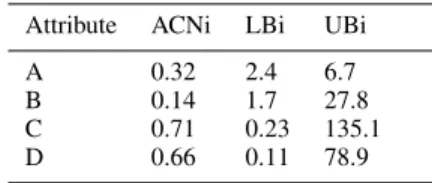
TABLE II
EXAPLE OFTHE RULEEXTRACTION Attribute ACNi LBi UBi
A 0.32 2.4 6.7
B 0.14 1.7 27.8
C 0.71 0.23 135.1 D 0.66 0.11 78.9
PSO weakness that it is often trapped in the local optimum; also, it is not robust when used on large datasets [8], [15].
Li et al., (2007), proposed a solution by using combination of the PSO method and the Cauchy distribution, which would help reach a wider and a more appropriate database by using the mutation process. In other studies e.g., Sangsawang (2015), this combination has the ability to optimize the two-stage reentrant flexible flow shop with blocking constraints. Furthermore, this combination improve the average solution by 15.60%. Therefore, the result of this combination is better than Hybrid Genetic Algorithm [16]. This combination was used subsequently to optimize the Integration of Process Planning and Scheduling (IPPS), and the results showed the reactive scheduling method and the effectiveness of the proposed IPPS method [17]. This method was evolved by Gen et al (2015) and Sangsawang (2015), to widen the search area in the process of mutation by using the Cauchy distribution. The result proved that the method could enhance the evolutionary process by widening search range. Based on these studies, we modified this method and solved the numerical problem for ARM optimization.
III. PROPOSEDMETHOD
A. The rule Extraction
The rules of numerical association rule mining by PARCD will be obtained by the particle representation procedure. This study used Michigan method which determine for every particle referring to one rule [5]. For wich the data set will be extracted into ACN category, based on the lower and upper bound value. Antecedent is pre condition and consequent is conclusion for describing a rule. The PARCD method can classify automatically the ACN based on the optimal threshold in every rules. This concept can be showed clearly by Table 1.
If the optimal procedure for one rule are 0 ACNi 0.33 for antecedent, 0.34 ACNi 0.66 for consequent and 0.67 ACNi 1.00 for none of them. For instance, see table 2. According to the table 2. The attribute A and B are the antecedent and the attribute D is consequent. The attribute C is not appearing
because it not includes both of them. Therefore, the rule is
AB!D.
B. Objective Design
This research uses several objective functions, i.e., support, confidence, and amplitude. The support measures the propor-tion of transacpropor-tions in D conceive X, or support(X)=|X|/ |D|. If X is the antecedent, the precondition then Y is consequence, the conclusion. Therefore, the support of the rule if X then Y is calculated as follow
Support(X[Y) =|X[Y |
|D| (1)
This support function is used to decide the confidence criterion. The confidence determine the quality of the rule referring the number of transactions in the all dataset. The rule that emerges in most transaction is assigned as a better quality [5].
Confidence(X[Y) = Support(X[Y)
Support(X) (2)
The amplitudes of attributes intervals, which fit to interest-ing rules, must be smaller [10]. Therefore, if two individuals have the similar number of records and attributes, the one having a smaller interval would provide better information. Therefore, the amplitudes of the intervals, which conform to the itemset and rule, are the minimization objectives.
Amplitude= 1 1
m⌃(i=1,m)
u
i li
max(Ai) min(Ai) (3)
Here,mis the number of attributes in the itemset,uiandli
are the upper and lower bounds which are encoded in the item-sets appropriate to the attribute, respectively, andmax(Ai)and min(Ai) are the allowable interval limits corresponding to
the attributes. Therefore, it is expected that rules with smaller intervals be produced [10].
C. PSO
The PSO method was discovered by Kennedy, an animal psychologist, and Eberhart, an electrical engineer, in 1995. They observed the swarming behaviors in flocks of birds, schools of fishes, or swarms of bees, and even in human groups [12].
The PSO method is initialized using a group of random particles (solutions); then, it searches for the optimal solution by updating generations. During all iterations, each particle is updated by following the twobestvalues. The first is the best solution (fitness) it has achieved so far; it is calledpBest. The other best value that is obtained by the PSO method is the best value in the population sphere; it is a global best (gBest). After finding the two best values, each particle updates its corresponding velocity and position [8], [12].
Each particle p, has a position x(t), and a displacement
velocity v(t) at some iteration t. The particle best (pBest)
memory. The velocity and position are updated using Eqs. 4 and 5, respectively [8], [12].
vi,new=!vi,old+c1rand()(pBest xi) +c2rand()(gBest xi)
(4)
xi,new =xi,old+vi,new (5)
Here!is the inertia weight;vi,newis particle velocity of the i-th particle after updating;xi is thei-th, or current particle; i is the particle number; rand() is a random number in the range (0, 1); c1 is the cognitif component; c2 is the social
component; pBest is the particle best; gBest is the global
best;xi,oldis the position of thei-th particle before updating;
andxi,new is the position of thei-th particle after updating or
from the current position citepLi2007a,Indira2014. D. Cauchy Distribution
The main equation of the probability density function (pdf) for the Cauchy distribution is shown in Eq. 6 [15].
f(x) = 1
s⇡(1 + ((x t)/s)2) (6)
The random variableY =F(X)has a uniform distribution
on [0,1). Consequently, if we invert F then it can use a
uniform density to simulate the random variable X, because X =F 1(Y). Therefore, the cumulative distribution function
of Cauchy distribution is F(x) = 1 ⇡arctan(x) + 0.5 (7) and therefore if y= 1 ⇡arctan(x) + 0.5 (8)
by inversing its function, the Cauchy random variable is
x=tan(⇡(y 0.5)) (9)
This function can also be written using Eq.10 because y has
a uniform distribution on [0,1). Hence,
x=tan(⇡/2·rand[0,1)) (10)
E. PSO for Numerical ARM Problem with Cauchy Distribu-tion (PARCD)
A limitation of the PSO method is that it does not gen-erate best solutions for large scale problems including high dimensional variables. The Cauchy distribution is used to deal with this problem. Therefore, it needs to make new mutation operations by using effective moving particles. A Cauchy PSO was proposed by Taichi (2014) for solving the multimodal optimization issue.
The PARCD method is proposed to solve the numerical problem of ARM [19]. This combination yields the best result
TABLE III PROPERTIES OFDATASETS
Dataset No. of Records No. of Attributes
Quakes 2178 4
Basketball 96 5
Body fat 252 15
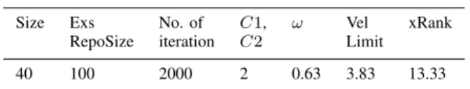
TABLE IV PARAMETERSETUP
Size Exs No. of C1, ! Vel xRank
RepoSize iteration C2 Limit
40 100 2000 2 0.63 3.83 13.33
because the limitation of PSO overcome by using Cauchy distribution. The wide searching using Cauchy distribution prevents the PSO from being trapped in the local optima.
vi(t+ 1) =!(t)vi(t) +c1rand()(pBest xi(t)) +c2rand()(gBest xi(t))
(11) The next step is the normalization process obtained by using the result ofvi(t+ 1). This step is used to make vector length
to be 1. The variant of Cauchy distribution is infinite and the scale of parameter is 1 [15]. ui(t+ 1) = vi(t+ 1) p vi1(t+ 1)2+vi2(t+ 1)2...+vik(t+ 1)2 (12) The result of the normalization process is then multiplied with the Cauchy random variable.
si(t+ 1) =ui(t+ 1)·tan ⇣⇡
2 ·rand[0,1)
⌘
(13) Then, the result of Eq.13, which is a combination of the velocity value and Cauchy distribution, is used to decide the new particle position.
xi(t+ 1) =xi(t) +si(t+ 1) (14)
IV. EXPERIMENTS ANDDISCUSSION
A. Experimental Setup
This experiment uses benchmark datasets from Repository of Bilkent University Function Approximation. Three datasets were used: Quake, Basketball and Body fat (Table 3). This experiment is organized on Intel Core i5, 8 GB main memory, running on Windows 7, and the algorithms are processed by using the Matlab software.
We first set up the values of some parameters of PARCD method, i.e., population size, external repository size, number of iterations,c1 andc2,!, velocity limit and xRank. They are
40, 100, 2000, 2, 0.63, 3.83, and 13.33, respectively [5] (table 4).
Fig. 2. Comparison of the support value
B. Experiments
The association rule analysis contains two steps. The first step is to determine the frequent itemset including the an-tecedents or consequences of each attribute. The second step is to implement the proposed algorithm. This research uses PARCD method.
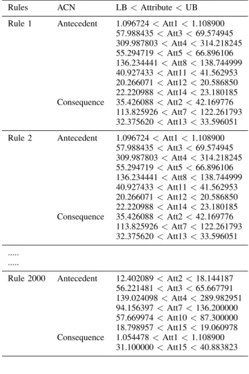
1) Rules Extraction of PARCD method: The result of the rules from the body fat dataset is one of the outputs, which is obtained by the PARCD method. Table 5 which depicts the complete parameter either antecedent or consequent. In the rule 1, we see that there are eight antecedent attributes and three consequent attributes, and these results are the same as in the rule 2. Then, in the last rule, rule 2000, the number of antecedent and consequent attributes are six and two, respectively.
The antecedent attributes in rule 1 are case number (Att1), percent body fat using Siri’s equation (Att3), density (Att4), age (Att5), adiposity index (Att8), chest circumference (Att11), abdomen circumference (Att12) and thigh circum-ference (Att14). Next, the consequent attributes are percent body fat using Brozek’s equation (Att2), height (Att7), and hip circumference (Att13). In rule 2, the antecedent and consequent attributes are the same as rule 1. Therefore, the rules 1 and 2 apply if (Att1, Att3, Att4, Att5, Att8, Att11, Att12, Att14) then (Att2, Att7, Att13). In the rule 2000, the antecedent attributes are percent body fat using Brozek’s equation (Att2), percent body fat using Siri’s equation (Att3), density (Att4), height (Att7), neck circumference (Att10), and knee circumference (Att15). Next, the consequent attributes are case number (Att1) and weight (Att6). Therefore, the rule 2000 applies if (Att2, Att3, Att4, Att7, Att10, Att15) then (Att1, Att6).
2) Comparison of PARCD and Other Methods: This part compares the result of the multi-objective function of the PARCD method with the other methods.
Figure 2 shows a comparison of the support value between PARCD and five previous methods (MOPAR, MODENAR, GAR, MOGAR, RPSOA). Generally, the support percentage of the PARCD method is higher than those of others. The support value of the Quake dataset is the lowest (22.97%)
TABLE V
RULES OF THEBODY FAT DATASET Rules ACN LB<Attribute<UB Rule 1 Antecedent 1.096724<Att1<1.108900
57.988435<Att3<69.574945 309.987803<Att4<314.218245 55.294719<Att5<66.896106 136.234441<Att8<138.744999 40.927433<Att11<41.562953 20.266071<Att12<20.586850 22.220988<Att14<23.180185 Consequence 35.426088<Att2<42.169776 113.825926<Att7<122.261793 32.375620<Att13<33.596051 Rule 2 Antecedent 1.096724<Att1<1.108900
57.988435<Att3<69.574945 309.987803<Att4<314.218245 55.294719<Att5<66.896106 136.234441<Att8<138.744999 40.927433<Att11<41.562953 20.266071<Att12<20.586850 22.220988<Att14<23.180185 Consequence 35.426088<Att2<42.169776 113.825926<Att7<122.261793 32.375620<Att13<33.596051 ... ...
Rule 2000 Antecedent 12.402089<Att2<18.144187 56.221481<Att3<65.667791 139.024098<Att4<289.982951 94.156397<Att7<136.200000 57.669974<Att10<87.300000 18.798957<Att15<19.060978 Consequence 1.054478<Att1<1.108900 31.100000<Att15<40.883823 Note :
ACN Antecedent, Consequent, None of them LB Lower Bound
UB Upper Bound Att1 Case Number
Att2 Percentage using Brozek’s equation Att3 Percentage using Siri’s equation Att4 Density
Att5 Age (years) Att6 Weight (lbs) Att7 Height (inches)(target) Att8 Adiposity index Att9 Fat Free Weight Att10 Neck circumference (cm) Att11 Chest circumference (cm) Att12 Abdomen circumference (cm) Att13 Hip circumference (cm) Att14 Thigh circumference (cm) Att15 Knee circumference (cm) Att16 Ankle circumference (cm) Att17 Extended biceps circumference (cm) Att18 Forearm circumference (cm) Att19 Wrist circumference (cm)
using the PARCD method, and the highest value is that of the MOPAR method (46.26%), and the remaining methods are just over 35% average. The support value of Basketball and
Fig. 3. The comparison of number of rules
Fig. 4. The comparison of confidence value
Body fat are the highest at 61.04% and 73.94%, respectively. The second position of the method for Basketball dataset is MOGAR (50.82%), and the average of other methods are well over 35%. The lowest support value for the Body fat dataset is the MOPAR method (22.95%) and the other averages are approximately 65%.
A comparison of the number of rules from the five methods are described in figure 3. The number of rules of the PARCD method was most similar to those of the others. The highest number of rules from Quake was MODENAR (55). The next, the highest from the Basketball dataset was PARCD (78); how-ever, in the Body fat dataset, this method performed the lowest (32). The MOGAR method had the highest performance.
Figure 4 provides a comparison of the confidence value. The confidence values of PARCD, MOPAR, and MOGAR are approximately the same, just over 80%. Generally, MOPAR has the highest confidence value in every dataset except for Body fat dataset where the MOGAR method is the highest one. Then, the second position is that of the PARCD method. Figure 2 and 4 show that support and confidence values have correlation with the number of rules. They have significantly negative correlation. If the support and confidence values are high, then the number of rules is low or reverse. This condition is because the high values of support and confidence selectively filter the number of rules.
Figure 5 and 6 reveal the size value and the percentage
Fig. 5. Comparison of the size values
Fig. 6. Comparison of the amplitude values
of amplitude of PARCD and other methods. Generally, the size value of the Body fat dataset is the highest for every method, especially for the GAR method, and is approximately 7.5. However, the size value of the Quake dataset using the MODENAR method is the lowest.
According to the amplitude result, the best value was provided by the PARCD method from the Basketball dataset; it was approximately 2% whereas the opposite value using the PARCD method with the Quake dataset gained approximately 65%. The amplitude value using the MOPAR method was fairly good; the Body fat dataset result was approximately 3%. The Quake dataset result was lower than that of the PARCD method, which was just over 50%. In addition, the other methods such as MODENAR, MOGAR, and GAR, showed better result than both the PARCD and MOPAR methods. Their amplitude results were approximately 17% to 29% in every dataset.
All the figures show that the PARCD method is better than the other methods, although in some cases, the result is less. This is because PARCD method contains a combination of PSO and Cauchy distribution, which empirically prevent the PSO from being trapped in the local optima. It proves that this combination is strong to solve some problems in different fields including the numerical problem for ARM optimization.
V. CONCLUSION
This study obtained the rule extraction by using hybrid of evolutionary algorithm, PSO and Cauchy distribution for solving the numerical ARM problem. The problems of local minimum and premature convergence in large datasets can be solved by using this combination. The experiment shows that the PARCD method in every multi-objective function, such as support, confidence, and amplitude gave better result than previous methods such as MOPAR, MODENAR, GAR, and RPSOA. For the future, the numerical problem of ARM can be further improved by developing or combining to other methods such as GA or Artificial Neural Network (ANN).
ACKNOWLEDGMENT
This paper was supported by various parties. We would like to thank the scholarship program from Kanazawa University, Japan and Ministry of Research, Technology and Higher Education (RISTEKDIKTI) and from STMIK AMIKOM Pur-wokerto, Indonesia. In addition, we thank for anonymous reviewers who gave input and correction for improving this research.
REFERENCES
[1] I. H. Witten, F. Eibe, and H. Mark A.,DATA MINING (Practical Machine Learning Tools and Techniques), vol. 3, no. 9. Elsevier, 2011.
[2] M. Almasi and M. S. Abadeh, Rare-PEARs: A new multi objective evolutionary algorithm to mine rare and non-redundant quantitative association rules, Knowledge-Based Syst., vol. 89, pp. 366384, Jul. 2015. [3] H. Jiawei, K. Micheline, and P. Jian, DATA MINING (Concept and
Techniques), vol. 3, no. 13. 2012.
[4] B. Minaei-Bidgoli, R. Barmaki, and M. Nasiri,Mining numerical asso-ciation rules via multi-objective genetic algorithms, Inf. Sci. (Ny)., vol. 233, pp. 1524, Jun. 2013.
[5] V. Beiranvand, M. Mobasher-Kashani, and A. Abu Bakar,Multi-objective PSO algorithm for mining numerical association rules without a priori discretization, Expert Syst. Appl., vol. 41, no. 9, pp. 42594273, Jul. 2014. [6] D. Arotaritei and M. G. Negoita,An Optimization of Data Mining Algo-rithms Used in Fuzzy Association Rules AlgoAlgo-rithms for Fuzzy Association Rules, V. Palade, R.J. Howlett, L.C. Jain KES 2003, LNAI 2774, pp. 980985, 2003.
[7] R. . c Alhajj and M. . Kaya,Multi-objective genetic algorithms based automated clustering for fuzzy association rules mining, J. Intell. Inf. Syst., vol. 31, no. 3, pp. 243264, 2008.
[8] C. Li, Y. Liu, A. Zhou, L. Kang, and H. Wang,A Fast Particle Swarm Optimization Algorithm with Cauchy Mutation and Natural Selection StrategyIsica 2007, pp. 334343, 2007.
[9] X. Yan, C. Zhang, and S. Zhang,Genetic algorithm-based strategy for identifying association rules without specifying actual minimum support, Expert Syst. Appl., vol. 36, no. 2, pp. 30663076, Mar. 2009.
[10] B. Alatas, E. Akin, and A. Karci,MODENAR: Multi-objective differen-tial evolution algorithm for mining numeric association rules, Appl. Soft Comput., vol. 8, no. 1, pp. 646656, Jan. 2008.
[11] H. R. Qodmanan, M. Nasiri, and B. Minaei-Bidgoli,Multi objective as-sociation rule mining with genetic algorithm without specifying minimum support and minimum confidence, Expert Syst. Appl., vol. 38, no. 1, pp. 288298, Jan. 2011.
[12] K. Indira and S. Kanmani, Association rule mining through adaptive parameter control in particle swarm optimization, Comput. Stat., vol. 30, no. 1, pp. 251277, 2014.
[13] V. Pachn lvarez and J. Mata Vzquez, An evolutionary algorithm to discover quantitative association rules from huge databases without the need for an a priori discretization, Expert Syst. Appl., vol. 39, no. 1, pp. 585593, Jan. 2012.
[14] K. N. V. D. Sarath and V. Ravi,Association rule mining using binary particle swarm optimization, Eng. Appl. Artif. Intell., vol. 26, no. 8, pp. 18321840, Sep. 2013.
[15] M. Gen; L. Lin; H.Owada,Hybrid Evolutionary Algorithms and Data Mining: Case Studies of Clustering, Proc. Soc. Plant Eng. Japan 2015 Autumn Conf., 2015.
[16] C. Sangsawang, K. Sethanan, T. Fujimoto, and M. Gen,Metaheuristics optimization approaches for two-stage reentrant flexible flow shop with blocking constraint Expert Syst. Appl., vol. 42, no. 5, pp. 23952410, 2015.
[17] Y. Xinjie and M. Gen,Introduction to Evolutionary Algorithms. Springer London Dordrecht Heidelberg New York, 2010.
[18] K. Taichi, Scatter Search Cauchy Particle Swarm Optimization for Multimodal Functions, J. Japan Ind. Manag. Assoc., vol. 64, no. 4, pp. 510518, 2014.
[19] I. Tahyudin and H. Nambo,The Combination of Evolutionary Algorithm Method for Numerical Association Rule Mining Optimization, in The Tenth International Conference on Management Science and Engineering Management, 2016, p. 1.