PAC-Bayesian Generalisation Error Bounds for Gaussian
Process Classification
Matthias Seeger [email protected]
Institute for Adaptive and Neural Computation University of Edinburgh
5 Forrest Hill, Edinburgh EH1 2QL, UK
Editor:Peter Bartlett
Abstract
Approximate Bayesian Gaussian process (GP) classification techniques are powerful non-parametric learning methods, similar in appearance and performance to support vector machines. Based on simple probabilistic models, they render interpretable results and can be embedded in Bayesian frameworks for model selection, feature selection, etc. In this paper, by applying the PAC-Bayesian theorem of McAllester (1999a), we prove distribution-free generalisation error bounds for a wide range of approximate Bayesian GP classification techniques. We also provide a new and much simplified proof for this powerful theorem, making use of the concept of convex duality which is a backbone of many machine learning techniques. We instantiate and test our bounds for two particular GPC techniques, includ-ing a recent sparse method which circumvents the unfavourable scalinclud-ing of standard GP algorithms. As is shown in experiments on a real-world task, the bounds can be very tight for moderate training sample sizes. To the best of our knowledge, these results provide the tightest known distribution-free error bounds for approximate Bayesian GPC methods, giving a strong learning-theoretical justification for the use of these techniques.
Keywords: Gaussian Processes, Generalisation Error Bounds, PAC-Bayesian Framework, Bayesian Learning, Sparse Approximations, Gibbs Classifier, Kernel Machines, Convex Duality.
1. Introduction
The Bayesian framework for probabilistic inference is widely used all over the statistics and machine learning communities, due to its high flexibility, its ability to render interpretable results and its conceptual simplicity. Within the framework, essential and difficult tasks like model and feature selection have canonical solutions. Complex models for real-world situations can be combined from simple, well-understood components in a structured way. Last, but not least, pitfalls hindering successful generalisation from finite data, such as over-fitting, can be tackled in a clear and principled way, so that Bayesian or approximate Bayesian solutions are typically among the top performers on difficult learning tasks. It is therefore of high theoretical and practical importance to analyse and understand the generalisation capability of (approximate) Bayesian methods. Many analyses so far have concentrated on the case where the true data distribution (stable aspects of which we try to learn) comes from a known family, which is either exactly the model family that the Bayesian method is using, or one which is close in some sense (e.g., Haussler and
Opper, 1997, Haussler et al., 1994, Sollich, 1999). Such analyses are important because they show up the principal limitations of the model family and the induction method, and because they often render close approximations to the true generalisation error we observe on independent test samples. However, they cannot give a guaranteed upper bound on the generalisation error (or other expectations of the true data distribution), because the validity of the whole analysis depends on assumptions that may not hold for the data distribution. PAC analyses1 of the generalisation capability of a learning technique provide such guaranteed bounds, in the sense that the probability of observing a violation of the bound is shown to be smaller than some a priori fixed δ > 0, where the probability is over random draws of the training sample from the true data distribution. We can hope to find such non-trivial bounds for finite training sample sizes, because we constrain the sampling process which generates the training set.2 Recently, a general result was obtained
by McAllester (1999a) which allows distribution-free analyses of competitive Bayesian or approximate Bayesian methods: thePAC-Bayesian theorem. In this paper, we show how to apply this result to approximate Bayesian Gaussian process classifiers (GPC), in order to obtain data-dependent PAC bounds for these powerful non-parametric methods. The PAC-Bayesian theorem and our results for GPC can be stated in simple and familiar terms and can be proved using elementary concepts only. Furthermore, experiments to be presented here indicate that our bounds can be very tight on real-world classification tasks with moderate training sample sizes, to an extent that they can provide practically meaningful generalisation error guarantees and may even be used for model selection in practice.
The structure of the paper is as follows. In the remainder of this section, we give a brief introduction to Gaussian process models for classification settings, together with fixing our notation. We also state McAllester’s PAC-Bayesian theorem, the backbone for our results, for which a simplified proof is given in Appendix A. In the following Section 2, we introduce the class of GP classification techniques we are interested in here and show how to apply the PAC-Bayesian theorem to any method from this class: this is our main result. In Section 3, we instantiate our main result for two particular GPC methods, namely Laplace GPC and sparse greedy GPC. The latter is of especially high practical significance due to its linear scaling with the training set size (our experimental results in Section 4.2 serve as demonstration of its impressive performance). Experimental results on a handwritten digits recognition task are presented in Section 4, testing our main result for the special GPC techniques discussed and comparing it to other state-of-the-art kernel classifier bounds. We close with a discussion in Section 5. The notation we use in this paper is summarised in Appendix B.
1.PACstands forprobably approximately correct, the framework was introduced by Valiant (1984). In this paper, we use the termPAC boundas synonym for “distribution-free large deviation bound”: a bound on the probability that an i.i.d. training sample gives rise to a large deviation between empirical and generalisation error. The bound is distribution-free, i.e. holds for any data distribution.
2. Typically, we assume that the training sample is drawn i.i.d. (independently and identically distributed) from the data distribution, but other less restrictive assumptions (e.g., Martingale sequences) are also possible.
1.1 The Binary Classification Problem. PAC Bounds
In the binary classification problem, we are given data S ={(xSi, tiS) | i= 1, . . . , n}, xi ∈
X, ti ∈ {−1,+1}, sampled independently and identically distributed (i.i.d.) from an
un-known data distribution over X × {−1,+1}. Our goal is to compute a classification
func-tion X → {−1,+1} from S which has small generalisation error on future test points
x∗, where (x∗, t∗) is sampled from the data distribution, independently of S. Given an
algorithm for computing such functions from samples S, we would like to construct a PAC upper bound on the generalisation error of this method. In the sequel, we denote
XS ={xSi |i= 1, . . . , n}, t= (tSi)i.
Data-independent (or uniform or a priori) PAC bounds ignore aspects of the learning algorithm other than the error of the selected classifier on the training set, and instead constrain the classification function to come from a restricted class of finite complexity in some sense. This restriction is donea priori, without looking at the sampleS, which allows the difference between empirical error (on S) and generalisation error (this difference is referred to as thegapin this paper) to be boundeduniformlyover all functions in the class, simply because the variability ofall functions is uniformly restricted. Vapnik-Chervonenkis theory (see Vapnik, 1998) essentially answers the question under which circumstances the gap converges uniformly to 0.
Uniform PAC bounds can answer questions about theoretical learnability of problems, however they are often extremely loose or even trivial in many practically relevant cases. There are two main reasons for this, apart from the distribution-free character of the PAC setting itself. First, the gap bounds do not depend on the observed sampleSat all. Whether the particular sampleS we encounter matches our prior assumptions or not does not influ-ence the bound value. Second, the gap bound value does not depend on the algorithm used to learn the predictor. It holds uniformly over all algorithms which select their classifica-tion funcclassifica-tion from the restricted class, even for a “maximally malicious” algorithm which, knowing the true data distribution, selects a function from the class which maximises the generalisation error, subject to a constraint on the empirical error onS. As a consequence, we either choose a very restricted classa priorito arrive at a small gap bound for reasonable
n, thus typically observing high empirical errors on a nontrivial task, or we live with a gap bound value which is trivial for all practically interesting sample sizesn. Both options are not tolerable from a practical viewpoint.
Data-dependent (or a posteriori) PAC bounds on the difference between empirical and generalisation error depend on the sample S. The idea is that prior knowledge about the unknown data distribution is used to introduce a weighting in the bounding technique which is biased towards our expectations. Namely, if it turns out that the data distribution matches our expectations rather closely, as judged by an empirical divergence measure which can be evaluated on the sample S, the gap bound value will be small (the lucky case).3 If
we are grossly wrong, the bound can be large, usually trivial. At this point, the notion of two differentsets of assumptions we are working with becomes most clear:
3. The concept of “luckiness” has been introduced to Statistical Learning Theory by Shawe-Taylor et al. (1998). We think that it is very much related to the concept of using prior distributions which penalise complex models (so-called “Occam’s Razor” priors); another good reason for applying PAC analysis to (approximate) Bayesian methods, in which luckiness can be formulated by the well-studied devices of modelling and prior assessment.
• In order to construct a classification method and a data-dependent bound for it, we follow Bayesian modelling assumptions: Available prior knowledge is encoded, within feasibility constraints, into a probabilistic model and prior distributions. The extent to which the unknown data distribution is compatible with these assumptions will in general determine the accuracy of the method and the observed tightness (yet not the validity) of the bound.
• The statement of the bound holds under standard PAC assumptions: We are given an i.i.d. training sample from the data distribution which is otherwise completely unknown.
Apart from the data dependency, our bound also concentrates only on the algorithm we are interested in. Even if this algorithm selects a classification function from some class or uses a mixture of such functions, the bound is specific to the way in which this is done. While a uniform bound merely suggests to select, from within the restricted class, a classifier which minimises the empirical error, in data-dependent bounds we have a trade-off between empirical error and the quality of the match between our prior assumptions and the classification function we construct. We know of no interesting real-world learning problem which comes without any sort of prior knowledge, and most of these problems are at least partly “non-malicious” in the sense that using this prior knowledge improves performance instead of deteriorating it. From this perspective, data-dependent bounds for specific algorithms are most promising for providing practically meaningful generalisation error guarantees.
1.2 The Approach. Gaussian Process Models
Recall from the previous subsection that in order to come up with a meaningful data-dependent PAC bound, we have to formalise our prior knowledge about the task in some concrete way, so that we can construct data-dependent complexity measures for the set of classification functions. The simplest way to do this is to modelthe relationshipx→t.
A binary classification model can be seen as a probabilistic formulation of the relations between the variables x → y → t, where the input variable x ∈ X, the latent output
y ∈ R and the observable target t ∈ {−1,+1}. Learning and generalisation works by assuming that the latent relationshipx →y is smooth and regular in some sense, however these regularities are obscured by noise; our task is then to separate the structure from the noise.4 Note that in this paper, we are interested only indiscrimination models, i.e. we do not attempt to model the data distribution over input points x. Distributions such as the data likelihood will always be conditioned on the corresponding input datapoints, although for simplicity this is not made explicit in the notation. Discrimination models typically are more robust and outperform complete models for the whole joint data distribution on tasks where the true input distribution cannot be identified well given the data. In general, a (discrimination) model is decomposed into some kind of family for the latent function x 7→y(x) and a classification noise model P(t|y). From the Bayesian viewpoint, y(·) is a
4. In this context, it is largely irrelevant whether there reallyexistsa smooth, underlying latent function. Being restricted to finite data, we cannot test such a hypothesis anyway. The perspective is positivistic: the model is “true” if we can use it to predict the future well.
random function, i.e., our knowledge about it will always remain uncertain to some extent. A common noise model is based on the Bernoulli distribution, withP(t|y) =σ(ty), where
σ(u) = (1 + exp(−u))−1 is the logistic function. Here, the latent function y(·) models the
logit log(P(t = +1|x)/P(t = −1|x)), which is why P(t|y) is often referred to as logit noise. Note that if, for a test point x∗, we knew the true logit ytrue(x∗), then the most
probable targett∗at x∗ is sgnytrue(x∗). Thus, a natural way to do classification within this
model-based framework is to estimate the latent function y(·) and then use the classifier x7→sgny(x). For more information about such discrimination models (see McCullach and Nelder, 1983, Green and Silverman, 1994).
The parametric modelling approach imposes a family of candidates{x7→y(x|w)}for
y(·), where w is a parameter vector, determining the function y(· |w). Examples are lin-ear models (i.e. y(x|w) = vTx+w0, w = (vT w0)T) or multi-layer perceptrons. If we
place a prior distribution P(w) on the parameter vector, the model is completely speci-fied and encodes our prior assumptions about the unknown data distribution. The non-parametric modelling approach differs from this, by placing a distribution directly ony(·), without assuming its membership in a fixed parametric family. Such a random process distribution is often constructed implicitly, by defining distributions over y(X) for every finite subset X ⊂ X. Here, we use the Matlab notation, i.e. if X = {x1, . . . ,xq}, then y(X) = (y(x1). . . y(xq))T. A Gaussian process (GP) is a random process y(·) over X
whose finite-dimensional marginal distributions are normal, i.e. for every finite set X ⊂ X
the corresponding random vector y(X) is Gaussian. Furthermore, marginalisation has to be consistent, in the sense that for two overlapping finite sets X1, X2, the marginal
dis-tributions of y(X1) and y(X2) on X1 ∩X2 have to be the same. The process is
essen-tially determined by a mean function m(x) = E[y(x)] and a covariance kernel K(x,x˜) = E[(y(x)−m(x))(y( ˜x)−m( ˜x))]. In the special casem(x)≡0, we refer toy(x) as azero-mean Gaussian process. Note that in this case,K(x,x˜) = E[y(x)y( ˜x)]. By placing a zero-mean Gaussian process prior on the latent functiony(·), we can specify a non-parametric model in which the choice of the kernelK encodes our prior assumptions about the unknown data distribution.5 Note that this definition of a GP is nothing more than the mathematically rigorous generalisation of a multivariate Gaussian random vector if X is infinite: vectors become functionsX →R, random vectors become random processes, and positive definite matrices become operators with positive definite kernels. In fact, for classification purposes we always condition on a finite number of input points from X and have to deal with finite-dimensional Gaussians only, yet the kernel is what associates observations with each other, allows us to generalise to future test points, draw decision boundaries, etc. For an introduction to Gaussian process models in the Bayesian context see (Williams, 1997). We will show in Section 2.1 how approximate Bayesian predictions for GP classification models can be obtained.
Let us finally introduce some notation. For two finite sets X1, X2 of input points, let
K(X1, X2) be the kernel matrix, i.e. K(X1, X2) = (K(x(1)i ,x (2)
j ))i,j, where x(k)i runs over 5. This prior is reasonable if we know that the classes have equal prior probability, as we will assume in this paper for simplicity. The general case can be treated by a straightforward parametric extension of the model, for which our results remain valid.
the points in Xk. Define K(X) =K(X, X). The kernel matrix over the training inputs is
denoted KS =K(XS). In the sequel, we will always assume thatKS is positive definite.6 1.3 The PAC-Bayesian Theorem
In this subsection, we introduce the PAC-Bayesian theorem of McAllester (1999a), where in this paper we restrict ourselves to the binary classification scenario.
Suppose we are given a function class {y(· |w)} parameterised by w. Many readers will be most familiar with this parametric formulation, however, note that w need not be a finite-dimensional vector. For example, in our application to non-parametric models below we will identifyw with the functiony(· |w) itself. In the binary classification setting defined in Section 1.1, it is understood thaty(x|w) predicts t(x) = sgny(x|w). A certain type of classifier, called Gibbs classifier, depends on the hypothesis class as well as on a distribution Q(w) over parameter vectors. Namely, given a test point x∗, the Gibbs
classifier predicts the corresponding target by first sampling w ∼ Q(w), then returning
t∗ = sgny(x∗|w), plugging in the parameter vector just sampled. Note that a Gibbs
classifier has a probabilistic element, i.e. requires coin tosses for prediction. Note also that if the targets of several test points are to be predicted, the parameter vectors sampled for this purpose are independent7. This is in contrast to the more familiar Bayes classifier which (in the case of our classification model) predicts t∗ = sgn E ∼Q[y(x∗|w)]. Another
type of rule, called Bayes voting classifier here, predicts t∗ = sgn E ∼Q[sgny(x∗|w)], i.e.
“votes” over classifiers sgny(x∗|w) instead of averaging discriminantsy(x∗|w).
McAllester’s PAC-Bayesian theorem deals with Gibbs classifiers for which the distribu-tionQ(w) may depend on the training sampleS, which is whyQ(w) is sometimes referred to as a “posterior distribution”. In order to eliminate the probabilistic element in the Gibbs classifier itself, the bound is on the gap between expected generalisation error and expected empirical error, where the expectation is over Q(w). The theorem can be configured by a prior distribution P(w) over parameter vectors, and the gap bound term depends most strongly on therelative entropy
D[QkP] = E ∼Q( ) logdQ(w) dP(w) (1) betweenQ(w) and the priorP(w). The relative entropy as a measure of deviation between two distributions is well-founded in information theory, statistics and many other fields (see Cover and Thomas, 1991). It arises naturally in maximum likelihood estimation and variational Bayesian approximations and is certainly one of the most important concepts in machine learning. Here, we assume that Q(w) andP(w) are absolutely continuous w.r.t.
6. It is possible to work with covariance kernels which have a non-zero null space and which can give rise to singular kernel matrices (for example spline kernels, see Wahba, 1990), however this requires the use of semi-parametric models which is not pursued here. Note that
S will typically have a numerical
ranksmaller thann, i.e. will often be ill-conditioned, and one has to be careful to employ appropriate numerically stable techniques.
7. Readers familiar withMarkov chain Monte Carlomethods will note the similarity with a MCMC approx-imation (based on one sample of only) of the corresponding Bayes classifier forQ( ). The difference
is that typically in MCMC, the sample representing the posterior Q( ) is retained and used for many
some positive measure, and dQ(w)/dP(w) is the Radon-Nikodym derivative (e.g., Ihara, 1993, Sect. 1.4) of Q(w) w.r.t. P(w). If Q(w) is not absolutely continuous w.r.t. P(w), i.e. if there is a null set of P(w) which is not a null set ofQ(w), we define D[QkP] =∞. Let us give some examples. If the mass of w is concentrated on a finite set of size L, say
{1, . . . , L}, the dominating measure is the counting measure, Q(w) and P(w) are finite distributions and D[QkP] = L X l=1 PrQ{w=l}log PrQ{w=l} PrP{w=l} . (2)
Ifw ∈Rm, the dominating measure is typically the Lebesgue measuredw, and D[QkP] = E ∼Q( ) logQ(w) P(w) .
Recall that for simplicity we use the same notation for a distribution and its density w.r.t.
dw, i.e. Q(w) = dQ/dw. For the formulation of Theorem 1, we require (as a special case of Equation 2) the relative entropy between two Bernoulli variables (skew coins) with probabilities of heads q, p, DBer[qkp] =qlog q p + (1−q) log 1−q 1−p. (3)
DBer is convex in (q, p), furthermore p7→DBer[qkp] is strictly monotonically increasing for p≥q, mapping [q,1) to [0,∞). Thus, the following function
D−1Ber(q, ε) =t s.t. DBer[qkq+t] =ε, t≥0 (4)
is well-defined for q∈[0,1) and ε≥0. We also define D−1Ber(q,∞) = 1−q. Note that, due to the convexity of DBer, we can compute D−1Ber(q, ε) easily using Newton’s algorithm. It is
clear by definition that for ε≥0, t∈[0,1−q):
t≥D−1Ber(q, ε) ⇐⇒DBer[qkq+t]≥ε. (5)
Suppose we are given an arbitrary prior distribution P(w) over parameter vectors, and we choose a confidence parameter δ∈(0,1). Then, the following result holds.
Theorem 1 (PAC-Bayesian theorem (McAllester, 1999a)) For any data distribution
over X × {−1,+1}, we have that the following bound holds, where the probability is over
random i.i.d. samples S ={(xSi, tiS)| i= 1, . . . , n} of size n drawn from the data distribu-tion:
PrS
gen(Q)>emp(S, Q) + D−1Ber(emp(S, Q), ε(δ, n, P, Q)) for someQ ≤δ. (6) Here,Q=Q(w) is an arbitrary “posterior” distribution over parameter vectors, which may depend on the sample S and on the prior P. Furthermore,
emp(S, Q) = E ∼Q( ) " 1 n n X i=1 I{sgny( S i | )6=tSi} # , gen(Q) = E ∼Q( ) E( ∗,t∗) I{sgny( ∗| )6=t∗} , ε(δ, n, P, Q) = 1 n D[QkP] + log n+ 1 δ .
Here, emp(S, Q) is the expected empirical error, gen(Q) the expected generalisation error of the Gibbs classifier based on Q(w) (note that the probability in gen(Q) is over (x∗, t∗)
drawn from the data distribution, independently of the sample S). D−1Ber(q, ε) is defined by (4), andD[QkP] denotes the relative entropy between the distributionsQandP, as defined in (1).
Note that McAllester’s theorem applies more generally to bounded loss functions and makes use of Hoeffding’s inequality for bounded variables. However, for the special case of zero-one loss, we can use techniques tailored for binomial variables which give considerably tighter results than Hoeffding’s bound if the expected empirical error of the Gibbs classifier is small. This version of McAllester’s theorem is proved in (Langford and Seeger, 2001). The proof of Theorem 1 we present here in Appendix A, is considerably simpler and more direct than the arguments used by McAllester (1999a) and McAllester (2002). It is based on the concept of convex duality which is itself a cornerstone of many techniques used in machine learning, such as the expectation maximisation algorithm, certain variational approximations to Bayesian inference and primal-dual optimisation schemes.
We should also stress once more, in accordance with what has been said in Section 1.1, that the PAC-Bayesian theorem does not require the true data distribution to be con-strained in any way depending on the prior P(w) and the model class. Other non-PAC analyses would probably require that the conditional data distribution is equal to
Q
iP(tSi |y(xSi,w∗)), w∗ ∼P(w∗), and under this restriction it might be possible to prove
stronger results than the PAC-Bayesian theorem (given that the model class is not too large).
1.3.1 Extension to the Bayes Classifier
In most situations in practice, when comparing Gibbs and Bayes classifier for the same posterior distributionQ(w) directly, it turns out that the Bayes variant can be computed more efficiently and often performs better than the Gibbs variant. Therefore, it would be of high interest to obtain a PAC-Bayesian theorem for Bayes classifiers as well. For fixed (x∗, t∗), define the errors of Gibbs, Bayes and Bayes voting classifiers as
eGibbs(x∗, t∗) = E ∼Q[I{sgny( ∗| )6=t∗}],
eBayes(x∗, t∗) = I{sgn E ∼Q[y( ∗| )]6=t∗},
eVote(x∗, t∗) = I{sgn E ∼Q[sgny( ∗| )]6=t∗}.
Furthermore, for A ∈ {Gibbs,Bayes,Vote}, define eA = E( ∗,t∗)[eA(x∗, t∗)] where the ex-pectation is over the data distribution. It is easy to relateeVote andeGibbs, by noting that if eVote(x∗, t∗) = 1, then eGibbs(x∗, t∗)≥1/2, thus eVote ≤2eGibbs (as remarked in Herbrich,
2001, lemma 5.3). The Bayes and the Bayes voting classifier are different rules in general, but in the special case that for each fixed (x∗, t∗), the distribution of y(x∗|w), w ∼Q is
symmetric around its mean, one can easily show that they are identical (thanks to Manfred Opper for pointing this out). Namely, fix x∗, write y∗=y(x∗|w), hy∗i= E ∼Q[y(x∗|w)]
and let u=y∗− hy∗i. The latter has a distribution which is symmetric with mean 0. Now,
the product of the predictions oft∗ by the Bayes and the Bayes voting variant is
sgn E [sgn (hy∗iy∗)] = sgn E
sgn hy∗i2+hy∗iu
which is 1 if hy∗i 6= 0. Since for hy∗i = 0, both variants predict sgn 0, we see that they
always predict the same t∗.
Combining these observations, we see that under the symmetry condition we have that
eBayes≤2eGibbs, thus in this case Theorem 1 applies to the Bayes classifier as well. However,
this is not really the result we are ideally looking for. Namely, given special distributional families forP andQ, we would like to obtain an analogue of Theorem 1 which results in a bound for eBayes which is the same or better than what we know foreGibbs, or at least no
more than 1 +εtimes theeGibbsbound, whereε1. Very recently, Meir and Zhang (2003)
obtained a strong PAC-Bayesian margin bound for the Bayes voting classifier, combining a new inequality based on Rademacher complexities with convex duality (as in our proof).
2. The PAC-Bayesian Theorem for Approximate Bayesian Gaussian Process Classification
In this section, we derive our main result: the application of the PAC-Bayesian Theorem 1 to a wide class of approximate Bayesian Gaussian process classification methods. We begin in Section 2.1 by introducing the Bayesian inference problem for binary GP classification and the class of approximate solutions we are interested in here. Methods in this class approxi-mate the true intractable predictive posterior process by a Gaussian one. In Section 2.2, we show how to compute the relative entropy (1) between such prior and posterior Gaussian processes. Finally, we state and discuss our main result (Theorem 2) in Section 2.3.
2.1 Approximate Bayesian Gaussian Process Classification
In this section, we introduce the Bayesian inference problem over GP classification models and the class of approximate methods which we are concerned with in this paper. This class is very broad and encompasses almost all Bayesian GPC approximations we know of. Given some data S with input points XS = {xSi |i = 1, . . . , n} and targets t = (tSi)i,
let yS =y(XS) ∈Rn. The Bayesian posterior distribution for yS is given by P(yS|S) ∝ P(S|yS)P(yS), where P(yS) =N(0,KS), KS =K(XS) by the GP prior, and
P(S|yS) =
n
Y
i=1
P(tSi |ySi), yS = (ySi )i
is the (conditional) likelihood. Unfortunately, due to the non-Gaussian noise distribution
P(t|y), it is in general intractable to work with the exact posterior P(yS|S) in order to do predictions. The class of approximations we are interested in here replaces P(yS|S) by a Gaussian distribution Q(yS|S). Once we have done this replacement, no further approximations are necessary, because the corresponding approximation of the predictive or posterior process turns out to be Gaussian as well. Namely, for any finite (ordered) set
X ⊂ X, let y = y(X). Now, by y \yS, we denote the (ordered) collection of variables obtained by deleting all components iny which correspond to input points ofX that occur inXS. yS\y is defined analogously. Now, define the distribution of y to be
Q(y|S) =
Z
Here, we follow the usual convention that densities over an empty set of variables are taken to be constant 1, and integrals over an empty set of variables are simply not done. This definition is a consequence of our data model, if we plug inQ(yS|S) forP(yS|S). Namely, first Q(y,yS|S) = P(y\yS|yS)Q(yS|S), from which we obtain (7) by integrating over yS \y. It is clear that Q(y|S) is Gaussian, and the consistency requirement can be checked straightforwardly, thus we have defined a Gaussian process approximating the true intractable posterior process, which can be used for (approximate) prediction as follows.
Suppose that
Q(yS|S) =N(yS|KSαˆS,ΣS) (8)
is the posterior approximation. Here, the parameters ˆαS ∈ Rn and ΣS ∈ Rn,n can be
chosen in an arbitrary way, given thatΣS andKS are positive definite. In order to predict y∗ = y(x∗) at a test point x∗, we need to compute Q(y∗|x∗, S) = N(y∗|µ(x∗), σ2(x∗)).
Let k(x∗) = K(XS,{x∗}). By computing the joint Gaussian P(y∗,yS) and conditioning
on yS, it is easy to see that
P(y∗|yS) =N(y∗|k(x∗)TK−1S yS, K(x∗,x∗)−k(x∗)TK−1S k(x∗)).
From this equation and (7) we see that y∗ ∼ Q(y∗|x∗, S) has the same distribution as r+k(x∗)TK−1S yS, wherer ∼N(r|0, K(x∗,x∗)−k(x∗)TK−1S k(x∗)) independent ofyS∼ Q(yS|S). Thus, by standard theorems of Normal theory (e.g., Mardia et al., 1979, Chap. 3), we arrive at
µ(x∗) =k(x∗)TαˆS, σ2(x∗) =K(x∗,x∗)−k(x∗)TMSk(x∗),
MS =K−1S −K−1S ΣSK−1S .
(9) The Equations (9) can typically be somewhat simplified for concrete ˆαS, ΣS (as chosen by
one of the approximate GPC methods we discuss below). Note that a predictive distribu-tion for the target t∗, i.e.Q(t∗|x∗, S), can be obtained by averaging the noise distribution P(t∗|y∗) overQ(y∗|x∗, S). This is a simple one-dimensional integral which can be
approx-imated using a numerical quadrature rule. The corresponding approximate Bayes classifier, i.e. the rule which chooses t∗ to maximise Q(t∗|x∗, S) is given by x∗ 7→ sgnµ(x∗), due to
the symmetry of Q(y∗|x∗, S) around its mean and the fact that P(t∗ = +1|y∗)−1/2 is
an odd function. This rule depends on the predictive mean µ(x∗) only, while it will turn
out below that the evaluation of the corresponding approximate Gibbs classifier requires the evaluation of σ2(x∗) as well. Thus, in the context of the GPC approximations we are interested in here, the Bayes classifier can usually be evaluated more efficiently than the Gibbs variant if extra information such asQ(t∗|x∗, S) is not required.
Approximation methods in the class we consider here differ in their choice of the pa-rameters ofQ(yS|S). Optimally, these parameters are chosen such that the true predictive process P(t∗|x∗, S) is closest to Q(t∗|x∗, S) in relative entropy. A more feasible choice
is, however, to match the predictive processes P(y∗|x∗, S) and Q(y∗|x∗, S) in this way,
which is equivalent to the maximum likelihood projection of P(y∗|x∗, S) onto the family
of Gaussian processes of the form shown in (7). The optimal choice of parameters requires matching of moments between P(yS|S) and Q(yS|S), and we can see from (9) that for this choice, the (approximate) Bayes classifier depends on the posterior mean of P(yS|S)
only. However, this mean is difficult to find (it can be approximated using MCMC sam-pling techniques, see Neal, 1997), and most approximations settle for other parameters of
Q(yS|S).
In the context of this paper, we are interested in the posterior Gibbs rather than the posterior Bayes classifier. The former predicts the target t∗ at a test point x∗ by sampling y∗ ∼ Q(y∗|x∗, S) from the approximate predictive distribution, then outputting sgny∗.
The expected error is given by
eGibbs(x∗, t∗) = Pry∗∼Q(y∗| ∗,S){sgny∗ 6=t∗}= Φ
−t∗µ(x∗)
σ(x∗)
, (10)
where Φ denotes the cumulative distribution function (c.d.f.) ofN(0,1).
Finally note that another frequently used way to introduce Gaussian process models is to view them as linear models with Gaussian prior distributions in a feature space which is typically infinite-dimensional. This view is very useful when designing new algorithms for approximate inference, since many ideas proposed originally for linear models can be imported rather straightforwardly. However, the feature space view requires a mathemati-cally rigorous treatment involving some functional analysis over so-called reproducing kernel Hilbert spaces, while working with Gaussian process models in the way introduced here is completely elementary. In this paper, we do not require the feature space view. We refer to (Williams, 1997) for a discussion of the relationships between the two views, and to (Wahba, 1990, Chap. 1) for the mathematical details required to establish the feature space view.
2.2 The Relative Entropy between Posterior and Prior Gaussian Process
In Section 1.2, we introduced Gaussian processes as distributions over random functions
y(·) : X → R, and in Section 2.1 we defined two Gaussian processes in particular: the zero-mean prior process P with covariance kernelK and the corresponding Gaussian pro-cess approximation Q to the true intractable posterior process, as given by (7) and (8). Our main result is an application of the general PAC-Bayesian Theorem 1 to approximate Bayesian GPC. For this non-parametric model, the parameter vector is the latent func-tion itself, i.e. w ≡y(·), and the prior P and posterior Q are the corresponding Gaussian process distributions. To this end, we need to compute the Radon-Nikodym derivative
dQ(y(·))/dP(y(·)) and the relative entropy term (1). It is easy to see that
dQ(y(·))
dP(y(·)) =
Q(yS|S)
P(yS) ,
whereyS=y(XS), the outputs over the training input points. Here,P(yS) =N(yS|0,KS),
and Q(yS|S) is given by (8). All we need to show is that the process defined by
dQˆ(y(·)) = Q(yS|S)
is a Gaussian process with the same parameters as Q. To see this, let X ⊂ X be finite and definey =y(X). Recall the notationsy\yS and yS\y from Section 2.1. Then we have
ˆ Q(y) = Z Q(yS|S) P(yS) P(y,yS)d(yS\y) = Z Q(yS|S)P(y\yS|yS)d(yS\y) =Q(y|S),
where the last equality uses (7). Therefore, the relative entropy D[QkP] is simply D[QkP] = Ey(·)∼Q logQ(yS|S) P(yS) = D[Q(yS|S)kP(yS)].
Since bothQ(yS|S) andP(yS) are Gaussians inRn, this is easily computed (e.g., Kullback, 1959): D[QkP] = 1 2log Σ−1S KS + 1 2tr Σ −1 S KS −1 +1 2αˆ T SKSαˆS− n 2. (11)
This formula depends of course on the parameters ˆαSandΣSof the posterior approximation Q(yS|S). In Section 3, we show how to compute the relative entropy for a range of concrete GPC approximations.
2.3 Main Result
In this section, we state and discuss our main result, namely an application of the PAC-Bayesian Theorem 1 to Gibbs variants of approximate PAC-Bayesian Gaussian process classifi-cation methods from the class introduced in Section 2.1. Examples for how this result looks like for several concrete methods are given in Section 3.
Choose some δ ∈ (0,1). Then, the following result holds for any zero-mean Gaussian process priorP with covariance kernel K.
Theorem 2 (PAC-Bayesian Theorem for GPC) For any data distribution over X × {−1,+1}, we have that the following bound holds, where the probability is over random i.i.d. samples S={(xSi, tS
i )|i= 1, . . . , n} of size n drawn from the data distribution:
PrS
gen(Q)>emp(S, Q) + D−1Ber(emp(S, Q), ε(δ, n, P, Q)) ≤δ. (12) Here, we have emp(S, Q) = 1 n n X i=1 Pryi∼Q(yi| S i,S) sgnyi 6=tSi , gen(Q) = E( ∗,t∗) Pry∗∼Q(y∗| ∗,S){sgny∗ 6=t∗}, ε(δ, n, P, Q) = 1 n D[QkP] + log n+ 1 δ .
Thus, emp(S, Q) is the expected empirical error, gen(Q) the expected generalisation er-ror of the GP Gibbs classifier (note that the probability in gen(Q) is over (x∗, t∗) drawn
from the data distribution, independently from the sample S) whose predictive distribu-tion Q(y∗|x∗, S) is given by (9), and D−1Ber(q, ε) is defined by (4). Finally, D[QkP] in ε(δ, n, P, Q) is given in (11). All of these terms depend on the parameters αˆS, ΣS of the
We have essentially already proved this theorem. In Section 2.1, we have shown how to compute the predictive distribution Q(y∗|x∗, S) (see Equation 9), thus emp(S, Q) can be
computed easily using (10). ε(δ, n, P, Q) is computed using (11). Below, when specialising to several concrete methods (i.e. “fill in” ˆαS andΣS), we will give more detailed comments on how to compute the terms the bound depends upon.
3. Applications to Concrete Gaussian Process Classification Methods
In the previous section, we stated and proved our main result (Theorem 2) which is valid for a large class of approximate Bayesian GPC techniques. In this section, we will instantiate this result with two particular GPC methods, both of high practical relevance. For these methods, which will both be introduced briefly, we provide computational details and some further analysis. The experiments presented in Section 4 are based on the GPC methods we describe here.
3.1 Laplace Gaussian Process Classification
In this section, we concentrate on a particular simple, yet powerful approximate GPC method suggested by Williams and Barber (1998). This technique is referred to asLaplace Gaussian process classification, and we will begin by briefly introducing this framework. A detailed introduction can be found in (Williams and Barber, 1998).
Recall from Section 1.1 that we are given some i.i.d. data sample S of size n, drawn from an unknown data distribution. Our noise model will be Bernoulli (logit), i.e.P(t|y) =
σ(ty), and for this non-Gaussian noise distribution, exact Bayesian analysis is intractable. In a nutshell, the Laplace GPC approximation works by first determining the vector ˆyS maximising the posterior P(yS|S), where yS = y(XS), XS = {xS1, . . . ,xSn}. This is a
convex optimisation problem, and therefore has a unique solution. Let KS =K(XS). In
our context, it is useful to operate on the dual vectorαS=K−1S yS. Then, the log posterior
can be written, up to additive constants, as a criterion
F(αS,KS) = n X i=1 logσ(tSi ySi)− 1 2α T SKSαS, yS= (ySi )i =KSαS. (13)
Since F is concave, it has a unique maximiser ˆαS which can be found using the Newton-Raphson algorithm. Furthermore, ˆyS =KSαˆSis the posterior mode. We now approximate the posteriorP(yS|S) by a GaussianQ(yS|S), using the Laplace approximation (e.g., Kaas and Raftery, 1995) around the mode ˆyS. This results in
Q(yS|S) =N(yS|KSαˆS,(W +K−1S )−1), (14) whereW is a diagonal matrix with positive entries. In fact, at the mode ˆyS, we have:
ˆ
αS = (tSiσ(−tiSyˆiS))i, W = diag(σ(−tSiyˆiS)σ(tSi yˆSi))i. (15)
Note that if ΣS = (W +K−1S )−1, then (14) becomes consistent with (8). If we define the
positive definite matrix
then some matrix algebra results in
MS=K−1S −K−1S ΣSK−1S =W1/2A−1W1/2, Σ−1S KS=W1/2AW−1/2.
(17) This allows us to compute the predictive distribution (9) and the relative entropy term (11) in a stable way. Suppose we are given the Cholesky decomposition (e.g., Horn and Johnson, 1985, Chap. 7) A = LLT, where L is lower-triangular with positive diagonal. Then, the predictive variance is computed as
σ2(x∗) =K(x∗,x∗)−rTr, Lr=W1/2k(x∗),
which is O(n2) due to the back-substitution for r. The Cholesky decomposition is by
far the most stable (and also most efficient) exact method to do these computations, and we discourage the reader from using other techniques involving matrix inversions. The evaluation of the expected empirical error emp(S, Q) in Theorem 2 requires the evaluation of the predictive variances at the training points, thus isO(n3).
Using (17), the relative entropy term (11) simplifies to D[QkP] = 1 2log|A|+ 1 2trA −1+1 2αˆ T SKSαˆS− n 2. (18)
Note that log|A| = 2 log|diagL|. The term trA−1 can be computed from L in roughly the same time asL is obtained fromA. Thus, the computation of (18) isO(n3) as well.
The Gibbs classifier seems unattractive for predictions on large test sets, because each evaluation requires O(n2). In contrast to this, the Bayes classifier variant depends on the meanµ(x∗) =k(x∗)TαˆS only, which is O(n) per test point. However, we show in (Seeger,
2002) how one can use sparse approximation techniques together with rejection sampling in order to avoid the exact computation of the variance term for most of the predictions, ending up withO(n) (average case) per prediction.
3.1.1 Some Analysis of the Relative Entropy Term
In this section, we present some analysis of the relative entropy term D[QkP] (see Equa-tion 18) in the bound of Theorem 2, as applied to Laplace GPC. In normal situaEqua-tions (i.e.
δ not extremely small), the expression ε(δ, n, P, Q) in (12) is dominated by this term. Now to the remaining terms in (18). The matrix A of (16) is positive definite, and all its eigenvalues are≥1. Furthermore, by taking any unit vector u and using the min-max characterisation of the eigenvalue spectrum (e.g., Horn and Johnson, 1985, Sect. 4.2) of Hermitian matrices, we have uTAu = 1 + (W1/2u)TKS(W1/2u) ≤ 1 +λmaxuTW u <
1 +λmax/4, where λmax is the largest eigenvalue of KS (note that the positive coefficients
of W are all < 1/4). Thus, all eigenvalues of A lie in (1,1 + λmax/4). By analysing
(1/2) log|A|+ (1/2) trA−1for general8 AIn, we see that this term must lie betweenn/2
and (n/2)(log(1 +λmax/4) + (1 +λmax/4)−1), although these bounds are not necessarily
tight.
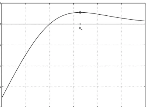
First, we can use (15) to show that ˆ αTSKSαˆS = ˆyTSαˆS = P itSiyˆSiσ(−tSiyˆiS), which is simply P if(tSiyˆiS), f(x) =x σ(−x), and tS
iyˆiS is the so-called margin at example
(xSi, tSi ). f(x) is plotted in Figure 1. It is maximal at x∗ ≈ 1.28, converges to 0
expo-nentially quickly for x→ ∞ and behaves like
x 7→ x for x → −∞. Thus, at least w.r.t. the third term in (18), classification mistakes (i.e. tS
iyˆSi < 0) render a negative
contribu-tion to the gap bound value. This is what we expect for a Bayesian architecture. Namely, the method chose a simple solution, at the expense of making this mistake, yet with the goal to prevent disastrous over-fitting. In our bound, we are penalised by a higher empirical error, but we should be rewarded by a smaller gap bound term.
−2 −1 0 1 2 3 4 −2 −1.5 −1 −0.5 0 0.5 margin x f(x) = x sigma(−x) x *
Figure 1: Relation between margin and gap bound part
3.2 Sparse Greedy Gaussian Process Classification
A principal drawback of many approximate GPC techniques in practice is their scaling of
O(n3) with the sample size n during training. For example, the Laplace GPC technique discussed in Section 3.1, although one of the fastest (non-sparse) known GPC techniques, scales asO(n3) in a straightforward implementation.9 Furthermore, these techniques
typ-ically require the evaluation of the complete kernel matrix KS. Recently, a number of sparse approximation techniques for Bayesian GPC have been proposed (e.g., Tipping, 2001, Williams and Seeger, 2001, Smola and Bartlett, 2001, Tresp, 2000, Csat´o and Opper, 2002, Lawrence, Seeger, and Herbrich, 2003), providing an important alternative for prac-titioners. The common theme of these techniques is to restrict the number of coefficients to be used in the final discriminant expansion to a controllable numberk n(an exception is the method of Williams and Seeger (2001) which results in a dense expansion). By means of this, some of these methods achieve a training complexity of at mostO(nk2). This involves the selection of a “representative” subset of size k of the training inputs. Since an optimal selection (in any meaningful sense) is intractable, the methods resort to randomised and/or greedy strategies, often of heuristic nature.
Here, we focus on a class of sparse GPC techniques proposed by Csat´o and Opper (2002) and Lawrence, Seeger, and Herbrich (2003). Due to space limitations, a detailed description of these methods cannot be given here, for details see (Seeger et al., 2002). In what follows, we introduce aspects of the methods we require in this section, but the exposition is not self-contained. We then show how the terms determining the bound value of Theorem 2 can be evaluated in timeO(nk2).
9. This is true for Laplace Gibbs GPC and for the evaluation of the terms determining the bound value in Theorem 2. Laplace Bayes GPC typically scales as O(n2
) (average case), if the Newton steps are approximated using a conjugate gradients solver.
The method falls in the class described in Section 2.1 and propagates Gaussian approx-imations Q(yS|S) to the intractable true posterior P(yS|S) (see Csat´o and Opper, 2002, Lawrence, Seeger, and Herbrich, 2003). Q(yS|S) is parameterised by a diagonal matrix Π
with nonnegative elements and a vector m:
Q(yS|S) =N yS|KS(In+ΠKS)−1TΠm,(K−1S +Π)−1,
whereT = diag(tSi )i contains the targets. This becomes consistent with (8) if we set ˆαS=
(In+ΠKS)−1TΠm and ΣS = (K−1S +Π)−1. In sparse variants of this approximation,
we allow for elements of diagΠ to be zero. In fact, for such methods we keep an active set I ⊂ {1, . . . , n}, with k = |I| n, and make sure that if diagΠ= (pi)i, then pi = 0
wheneveri6∈I. The active set is grown up to a desired size (or until a stopping criterion is met) byincludingnew datapoints (xSi, tSi ). In order to include a new pointi, the algorithm only requires thei-th row of the kernel matrix KS, i.e.K({xSi }, XS). After I has reached
the desired size, the method can be stopped, but some variants try to continue to refine the approximation while keeping the size ofI constant. Insparse greedy variants of this scheme, the next datapoint to be included is selected greedily using a heuristic scoring criterion. In this work, we employ the heuristic proposed in (Lawrence, Seeger, and Herbrich, 2003), referred to asdifferential entropy score, which can be evaluated very efficiently.10 The first few patterns to be included are chosen at random. Later, we select a pattern by scoringall remaining ones using the differential entropy criterion and pick the winner. The algorithm stops once k patterns have been included.
Due to the fact that at most k of the elements in diagΠ are non-zero, it turns out that the quantities depending on the final posterior approximation Q(yS|S) which we are interested in, namely the parameters of the predictive distribution (9) and the relative entropy term (11) can be computed efficiently and using only the part [KS]I,·of the kernel
matrix. First note that
MS = (In+ΠKS)−1Π, Σ−1S KS =In+ΠKS.
Denote Πk= [Π]I,I and define
B=Ik+Π1/2k [KS]I,IΠ1/2k ∈Rk×k, β=Π1/2k B−1Πk1/2[T m]I ∈Rk.
If EI ∈ Rk,n denotes the “selection” matrix for I, i.e. EIg = [g]I, then some elementary
matrix algebra using the Sherman-Morrison-Woodbury formula (e.g., Press et al., 1992, Sect. 2.7) gives (In+ΠKS)−1=In−ETIΠ 1/2 k B−1Π 1/2 k [KS]I,IEI, MS = Π1/2k EI T B−1Π1/2k EI. (19)
10. We remark that although the schemes proposed in (Csat´o and Opper, 2002) and (Lawrence, Seeger, and Herbrich, 2003) seem quite similar, in that they include new datapoints into the approximation in the same way, they are algorithmically quite different. The method proposed by Csat´o and Opper (2002) is an on-line scheme in which datapoints are used to refine the posterior approximation even ifthey are not included into the active set, while this does not hold for the method suggested in (Lawrence et al., 2003). This means that the latter can be significantly faster, yet less accurate in practice, although both methods scale as O(nk2
). Furthermore, the greedy method is a compression scheme (see Section 4.3), which is not the case for the on-line algorithm.
Since ˆαS =MST m, we have ˆαS =ETIβ. The predictive variance is best computed using the Cholesky decomposition B=LkLTk. Plugging (19) into (9), we have
µ(x∗) =βTkI(x∗), σ2(x∗) =K(x∗,x∗)−rTr, Lkr=Π1/2k kI(x∗),
where kI(x∗) = (K(x∗,xSi))i∈I ∈ Rk. Thus, each Gibbs prediction can be computed in O(k2), and the expected empirical error of the Gibbs classifier is obtained at a cost of O(nk2). Note that the corresponding Bayes classifier can be evaluated in O(k), due to the sparse expansion for µ(x∗). For the computation of the relative entropy term (11), we use
(19) and the well-known matrix formulas |I+U V|=|I +V U| and trU V = trV U (the former follows from a well-known formula using Schur products, e.g., Horn and Johnson, 1985, Sect. 0.8.5). Then, log|Σ−1S KS| = log|B| and tr(Σ−1S KS)−1 = n−k + trB−1,
therefore D[QkP] = 1 2log|B|+ 1 2trB −1+ 1 2β T [K S]I,Iβ− k 2. (20)
This is computed in O(k3), given the Cholesky decomposition of B. All in all, the upper bound on gen(Q) given by Theorem 2 for sparse greedy GPC can be computed inO(nk2).
It is interesting to point out the close similarity between the two relative entropy formulas (18) and (20). This is due to the similar form of ΣS (covariance matrix of Q(yS|S)) both
methods are employing, namely ΣS = (K−1S +D)−1, where D is a diagonal matrix. In
the Laplace GPC case, withD =W, the components of diagD are positive, and there is no force which drives many of these components towards zero. In the sparse greedy GPC case, with D = Π, n−k of the components of diagD are zero, allowing us to use more efficient computations. Note that the method we have discussed in this section becomes identical to the “cavity” approach suggested by Opper and Winther (2000) if we let k=n, i.e. allow all components ofΠto become non-zero (see also Minka, 2001). Another idea to control sparsity inΠ, different from the approaches in (Csat´o and Opper, 2002, Lawrence, Seeger, and Herbrich, 2003), would be to place special priors on the components of Π, forcing them to be small under the posterior if the data does not suggest otherwise. This is the approach adopted by the relevance vector machine (RVM)of Tipping (2001), although there the sparsity of a set of parameters different from Πis controlled.
We would also like to remark that our bound for sparse greedy GP methods is (in general) not a compression bound. Theorems of the latter class require that the finally selected discriminant is exactly recovered if we restrict ourselves, in an independent training run, to the datapoints in the final expansion as a training set (see Section 4.3). Although our bound applies to compression scheme versions of sparse greedy GPC, it is not restricted to such. The experiments presented in Sections 4.2 and 4.3 suggest that Theorem 2 for sparse greedy GPC renders a much tighter generalisation error bound than a standard PAC compression bound in situations where both bounds apply.
4. Experiments
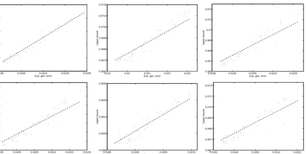
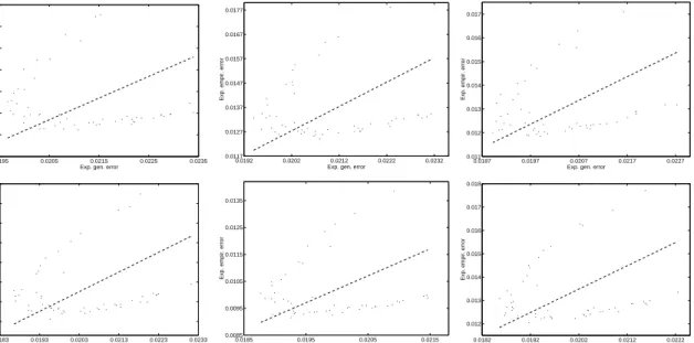
Here, we present experiments testing our main result (Theorem 2) for the Laplace GP Gibbs classifier of Section 4.1 and the sparse greedy GP Gibbs classifier of Section 4.2, using a setup to be described shortly. The results indicate that the bounds are very tight even for
training samples of moderate sizes. In Section 4.3, we compare our bound to a state-of-the-art PAC compression bound for the sparse greedy GP Bayes classifier, and to the same compression bound for the soft-margin support vector classifier in Section 4.3.1. Finally, in Section 4.4 we try to evaluate the model selection qualities of our result for sparse greedy GP classification.
A real-world binary classification task was created on the basis of the well-known MNIST handwritten digits database11 as follows. MNIST comes with a training set of 60000 and a test set of 10000 handwritten digits, represented as 28-by-28-pixel bitmaps, the pixel intensities are quantised to 8 bit values. First, the input dimensionality was reduced by cutting away a 2-pixel margin, then averaging intensities over 3-by-3-pixel blocks, resulting in 8-by-8-pixel bitmaps. The task of discriminating handwritten twos against threes is among the harder binary ones.12 By selecting these digits only, a training pool of 12089 cases and a test set ofl= 1000 cases were created.
For our experiments, we employed the frequently used Radial Basis Functions (RBF) covariance kernel K(x(1),x(2)) =Cexp −w 2d x (1)−x(2) 2 .
Here, d is the dimensionality of the inputs (d = 64 in our case), w and C are positive parameters. C determines the variance of the underlying random process (see Section 1.2), while w−1/2 determines its average length scale.
The experimental setup is as follows. An experiment consists of L = 10 independent iterations. During an iteration, three datasets are sampled independently and without replacement from the training pool: a model selection (MS) training set of size nMS, a
MS validation set of size lMS and a task training sample S of size n. Note that the latter
set is sampled independently from the model selection sets, ensuring that the prior P in Theorem 2 is independent of the task training sample. This issue is discussed in more detail in Section 5. Then, model selection is performed over a list of candidates for (w, C), where a classifier is trained on the MS training set and evaluated on the MS validation set (the MS score is the expected empirical error of the Gibbs classifier on the MS validation set). The winner is then trained on the task training set and evaluated on the test set. Alongside, the upper bound value given by Theorem 2 is evaluated, where the confidence parameter δ is fixed to 0.01. We also quote total running time, as observed on a DEC Alpha workstation with almost four gigabytes of RAM.
4.1 Experiments with Laplace GPC
Our implementation uses the Newton-Raphson algorithm in order to maximise the log posterior criterion (13). The Newton steps are computed using a conjugate gradients solver for symmetric positive definite linear systems. The prediction vector ˆαS is found inO(n2) (average case). The Cholesky decomposition of the system matrix (16), the evaluation of the expected empirical error of the Gibbs classifier and of the relative entropy term (18) require O(n3) each. The specifications and results for the experiments of this section are
11. Available online athttp://www.research.att.com/∼yann/exdb/mnist/index.html.
listed in Table 1. For all these experiments, we chose model selection validation set size
lMS= 1000 (recall that the test set is fixed with sizel= 1000). Experiments #1 to #5 have
growing sample sizes n = 500,1000,2000,5000,9000, the corresponding MS training set sizes are nMS = 1000 for experiments #2 to #5, andnMS= 500 for experiment #1. Note that nMS < nin experiments #3 to #5 is chosen for computational feasibility, due to the
considerable size of the candidate list for (C, w). In Table 2, we list additional information about the experiments.
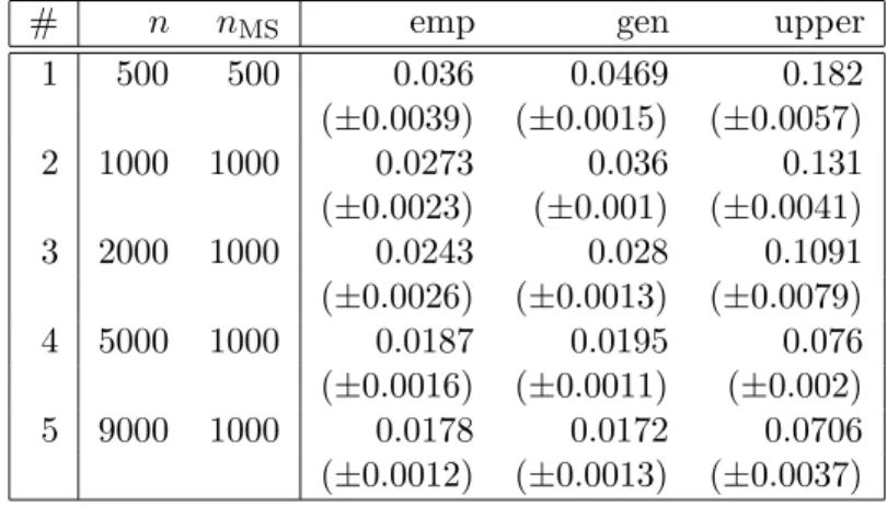
# n nMS emp gen upper
1 500 500 0.036 0.0469 0.182 (±0.0039) (±0.0015) (±0.0057) 2 1000 1000 0.0273 0.036 0.131 (±0.0023) (±0.001) (±0.0041) 3 2000 1000 0.0243 0.028 0.1091 (±0.0026) (±0.0013) (±0.0079) 4 5000 1000 0.0187 0.0195 0.076 (±0.0016) (±0.0011) (±0.002) 5 9000 1000 0.0178 0.0172 0.0706 (±0.0012) (±0.0013) (±0.0037)
Table 1: Experimental results for Laplace GPC. n: task training set size; nMS: model
selection training set size. emp: expected empirical error; gen: expected generali-sation error (estimated as average over test set). upper: upper bound on expected generalisation error after Theorem 2. Figures are mean and width of 95% t-test confidence interval.
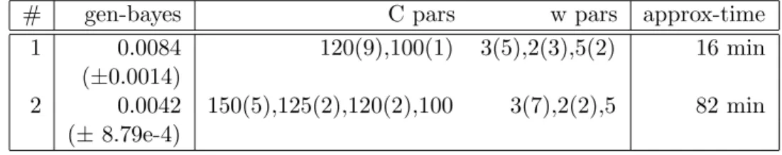
# gen-bayes C pars w pars approx-time
1 0.0339 50(6),30(2),20,25 0.5(5),2(3),0.75(2) 14 min (±0.0023) 2 0.0274 10(9),20 3(5),2(2),5 67 min (±0.0022) 3 0.0236 5(5),3(3),10(2) 10(6),7.5(2),5(2) 91 min (±0.0029) 4 0.0171 5(6),7.5(2),15,20 7.5(3),10(3),12(2),5,3 762 min (±0.0016) 5 0.0158 2(4),3(2),5(2),7.5(2) 12(4),10(3),5(2),7.5 3618 min (±0.0017)
Table 2: Additional information for Laplace GPC experiments. gen-bayes: test error of corr. Bayes classifier. C pars, w pars: Values of C, w chosen by MS (frequency in parentheses). approx-time: approximate total running time. Figures are mean and width of 95%t-test confidence interval.
Note that the resource requirements for our experiments are well within today’s desktop machines computational capabilities. For example, experiment #4 was completed in total time of about 12 to 13 hours, the memory requirements are around 250M. Now, for this setting both the expected empirical error and the estimate (on the test set) of the expected generalisation error lie around 2%, while the PAC bound on the expected generalisation error given by Theorem 2 is 7.6% — an impressive, highly nontrivial result on samples of size
n= 5000. Our largest experiment #5 was done mainly for comparison with experiment #2 for sparse greedy GPC (see Section 4.2). The total computation time was 6 hours for each iteration, and the memory requirements are around 690M. We note a slight improvement in test errors as well as in the upper bound values (which now lie around 7%).
The “gen-bayes” column in Table 2 contains the test error that a Bayes classifier with the same approximate posterior as the Gibbs classifier attains. Note that it is not necessarily the best we could obtain for a Bayes classifier, because the model selection is done specifically for the Gibbs, not the Bayes classifier. In the Laplace GPC case we note that Bayes and Gibbs variants perform comparably well, although the Bayes classifier attains slightly better results and, as mentioned in Section 2.1, can be evaluated more efficiently. We include these results for comparison only: although our main result implies a bound on the generalisation error of the Bayes classifier (see Section 1.3.1), the link is too weak to render a sufficiently tight result.
4.2 Experiments with Sparse Greedy GPC
The algorithmic details of our implementation can be found in a separate paper (Seeger et al., 2002). Training proceeds in two phases. In the first phase, a numberkrand of patterns
from the training sample are selected at random and included into the approximation. In the second phase, we include further patterns until the active set has grown to size k. However, now the next pattern to be included is determined by scoring all remaining ones using the differential entropy criterion (see Section 3.2) and choosing the one with the best value. Empirically, we found the greedy selection to be very effective, thus typically
krand k. Note that we require krand ≥ 1, because the differential entropy criterion is
constant over all patterns if the active set is empty and the kernel diagonal is constant. We use different values for k and krand during model selection, denoted by kMS, krand,MS.
For all experiments reported here, we chose MS training size nMS = 1000, MS validation
size lMS = 1000, kMS = 150, krand = 3 and krand,MS = 2. Note that in experiments which
have the same (n, nMS, lMS) constellation as Laplace GPC experiments, we use the same
data subsets, in order to facilitate direct comparisons. The results are listed in Table 3. In Table 4, we list additional information about the experiments.
Let us compare these results to the ones obtained for Laplace GPC. The sparse GPC Gibbs classifier trained with 5000 examples attains an expected test error of 2.1%, and the upper bound evaluates to 6.7%. While the former is the same as for the Laplace GPC variant, the latter is significantly lower. The ratio between upper bound and expected test error is 3.19, the ratio between gap bound and expected test error is 2.46 — demonstrating an impressive tightness for a state-of-the-art classifier trained on just 5000 examples. Also important for the practitioner, experiment #1 for the sparse GPC was completed in total time of about 16 minutes on the machine mentioned in Section 4.1 — almost fifty times faster
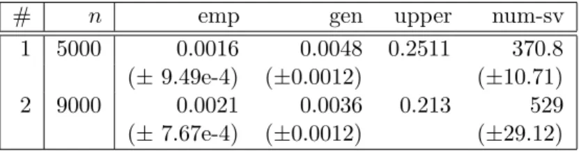
# n k emp gen upper
1 5000 500 0.0154 0.0207 0.067
(±0.0021) (±0.0015) (±0.0026)
2 9000 900 0.0101 0.0116 0.0502
(± 6.88e-4) (±5.49e-4) (±6.13e-4)
Table 3: Experimental results for sparse GPC.n: task training set size; k: final active set size. emp: expected empirical error; gen: expected generalisation error (estimated as average over test set). upper: upper bound on expected generalisation error after Theorem 2. Figures are mean and width of 95%t-test confidence interval.
# gen-bayes C pars w pars approx-time
1 0.0084 120(9),100(1) 3(5),2(3),5(2) 16 min
(±0.0014)
2 0.0042 150(5),125(2),120(2),100 3(7),2(2),5 82 min (±8.79e-4)
Table 4: Additional information for sparse GPC experiments. gen-bayes: test error of corr. Bayes classifier. C pars, w pars: Values of C, w chosen by MS (frequency in parentheses). approx-time: approximate total running time. Figures are mean and width of 95%t-test confidence interval.
than the Laplace GPC experiment #4. Note that the limited size of the task database does not allow samples sizes much larger than n= 9000 (experiments on much larger datasets are subject to future work). It is interesting to observe that for this sample size, the results here are significantly better than for the full Laplace GPC on the same task13 (experiment #5 in Section 4.1). Finally note that we did not try to optimise the final active set sizek, but simply fixed k=n/10 a priori. An automatic choice of k could be based on heuristics which evaluate the error on the datapoints outside the active set.
The “gen-bayes” column in Table 4 serves the same purpose as the “gen-bayes” column in Table 2. In case of sparse greedy GPC, the results show that the Bayes classifier performs somewhat significantly better than the Gibbs variant, although the latter still attains very competitive results. A possible explanation for this difference, given that it cannot be observed for Laplace GPC, is obtained by inspecting the (C, w) kernel parameters values that are preferred by sparse greedy GPC. The parameterC is much larger for sparse GPC, i.e. the latent process has a larger a priori variance. This is sensible, because sparse GPC has to rely on much fewer terms in the final expansion than Laplace GPC, thus has to make sure that the kernels corresponding to active patterns span a larger range, and also
13. Note that we are comparing two entirely different ways of approximating the true posterior by a Gaussian: a Laplace approximation around the mode (which is different from the posterior mean — the “holy grail” of Bayesian logistic regression, see Section 2.1) and an approximation based on repeated moment matching. A more meaningful direct comparison would involve the TAP method of Opper and Winther (2000) which is, however, significantly more costly to compute than the Laplace approximation.
the coefficients in the expansion (the coefficients of β) lie in a broader interval. However, this typically leads to an increase in the predictive variances, which in turn might introduce more sampling errors in the Gibbs predictions.
4.3 Comparison with PAC Compression Bound
In this section, we present further experiments in order to compare our result for sparse GPC with a state-of-the-artPAC compression bound. Note that here, we employBayesGP classifiers instead ofGibbsGP classifiers: it would not be fair to compare our Gibbs-specific bound to an “artificially Gibbs-ified” version of a result which is typically used with Bayes classifiers. A compression bound applies to learning algorithms which have a particular characteristic. Namely, suppose we are given a learning algorithm A which maps data samplesS of size nto hypothesesA(S), which are then used to classify future input points.
A is called a compression scheme if there exists another algorithm R, mapping samples of size smaller than nto hypotheses, such that for every sample S we can find a k < nand a subsample ofSof sizeksuch thatRtrained on this subsample outputs the same hypothesis asA trained on S. Popular examples of compression schemes are the perceptron learning algorithm of Rosenblatt (1958) and the support vector machine (see Section 4.3.1).
It turns out that the sparse greedy GPC variant we are using in the experiments re-ported in Section 4.2, is a compression scheme where k is fixed a priori. Herbrich (2001, Theorem 5.18) gives a PAC bound for compression schemes (drawing from earlier work of Littlestone and Warmuth, 1986) which can be considered state-of-the-art. In order to en-sure a fair comparison, we use a refined version of this bound which can be found in (Seeger, 2002). There, it is also shown why and to what extent our sparse greedy GPC variant is a compression scheme. The PAC upper bound on the generalisation error depends only on the training error on the remainingn−kpatterns ofSoutside the active set (called emp\k(S)),
furthermore on k and krand. We repeated the experimental setup used in Section 4.2 and
employed the same dataset splits. The results can be found in Table 5.
# n k emp gen upper
1 5000 500 0.0025 0.0058 0.3048 (±6.79e-4) (±0.0015) (±0) 2 9000 900 0.0024 0.003 0.3041 (±4.25e-4) (±7.54e-4) (±0)
Table 5: Experimental results for PAC compression bound with sparse GP Bayes classifier.
n: task training set size; k: final active set size. emp: empirical error (on full training set); gen: error on test set. upper: upper bound on generalisation error given by PAC compression bound. Figures are mean and width of 95% t-test confidence interval.
For both experiments, emp\k(S) = 0 was achieved in all runs, the compression bound is tightest in this case. Nevertheless, in experiment #1, the upper bound on the generalisation error is 30.5%, a factor of 50 above our estimate on the test set. The ratio is even worse for experiment #2.
The reader may wonder why the generalisation errors here are slightly lower than the ones reported in Table 4. This should be due to the fact that in Section 4.2, we evaluated the Bayes classifier based on the hyperparameter values which have been optimised for the Gibbs variant, while here we performed model selection for the Bayes classifier explicitly.
4.3.1 Comparison with Compression Bound for Support Vector Classifiers
We can also compare our main result for sparse GP Gibbs classifiers with state-of-the-art bounds for the popular support vector machine (SVM). This kernel machine is non-probabilistic, due to its ε-insensitive loss which cannot be seen as the negative log of a proper noise distribution (see Seeger, 2000). A trained SVM discriminant function is a ker-nel expansion much like the discriminant function of a GP Bayes classifier (the predictive mean). The special form of the loss function encourages sparse expansions on tasks which are not very noisy. The training patterns corresponding to non-zero dual expansion coeffi-cients are referred to as support vectors. However, sparseness is not a directly controllable parameter, furthermore it is not an explicit algorithmic goal of the SVM algorithm to end up with a maximally sparse expansion. The aim is rather to maximise the “soft” minimal empirical margin which is, loosely speaking, the minimal empirical margin (i.e. the distance of the discriminating hyperplane to the closest datapoints, as measured in the feature space norm) after removing some outlier training points (we are penalised for the margin vio-lations of these outliers). This particular statistic of the empirical margin distribution is inspired by some PAC generalisation error bounds (e.g., Shawe-Taylor et al., 1998, Herbrich and Graepel, 2001), but in our opinion this link is rather weak for “non-near-asymptotic” situations. In practice, modern algorithms for SV classification such as Sequential Minimal Optimisation (SMO)proposed by Platt (1998) can often tackle problems with rather large sample sizesnin much less thanO(n3) (average case), by concentrating optimisation efforts
on a small active set. For more details on SVM see (Vapnik, 1998, Burges, 1998, Cristianini and Shawe-Taylor, 2000, Sch¨olkopf and Smola, 2002, Herbrich, 2001). Due to the setup of SVM training as a constrained optimisation problem, it is possible to show that the algo-rithm is a k-compression scheme, where k is the number of support vectors. Thus, if we observe a small ratio k/n, the PAC compression bound will render a nontrivial guarantee on the generalisation error. It is important to observe that in case of SV classification, we always have emp\k(S) = 0, i.e. the trained discriminant does not make any errors on the points which are not support vectors, and that this zero-error case is maximally favourable to the PAC compression bound. Experimental results for SV classifiers and the PAC com-pression bound can be found in Table 6. Again, we employed the same dataset splits as used in Section 4.2.
In both experiments, a higher degree of sparsity is attained than the one chosen in the experiments above for sparse GPC (as mentioned above, we did not try to optimise this degree in the sparse GPC case), leading to somewhat better values for the PAC compression bound. However, the values of 25% (experiment #1) and 21% (experiment #2) are still by factors > 50 above the estimates computed on the test set. The compression bound applies to SVM, but is certainly not specifically tailored for this algorithm, since it does not even depend on the empirical margin distribution. The margin bound of Shawe-Taylor et al. (1998), commonly used to justify data-dependent structural risk minimisation for