Department of Econometrics and Business Statistics
http://www.buseco.monash.edu.au/depts/ebs/pubs/wpapers/
Automatic forecasting with a
modified exponential smoothing
state space framework
Alysha M De Livera
April 2010
exponential smoothing state space
framework
Alysha M De Livera
Department of Econometrics and Business Statistics, Monash University, VIC 3800
Australia.
Email: [email protected]
Division of Mathematics, Informatics and Statistics,
Commonwealth Scientific and Industrial Research Organisation, Clayton, VIC 3168
Australia.
Email: [email protected]
28 April 2010
exponential smoothing state space
framework
Abstract
A new automatic forecasting procedure is proposed based on a recent exponential smoothing framework which incorporates a Box-Cox transformation and ARMA residual corrections. The procedure is complete with well-defined methods for initialization, estimation, likeli-hood evaluation, and analytical derivation of point and interval predictions under a Gaussian error assumption. The algorithm is examined extensively by applying it to single seasonal and non-seasonal time series from the M and the M3 competitions, and is shown to provide competitive out-of-sample forecast accuracy compared to the best methods in these competi-tions and to the traditional exponential smoothing framework. The proposed algorithm can be used as an alternative to existing automatic forecasting procedures in modeling single seasonal and non-seasonal time series. In addition, it provides the new option of automatic modeling of multiple seasonal time series which cannot be handled using any of the existing automatic forecasting procedures. The proposed automatic procedure is further illustrated by applying it to two multiple seasonal time series involving call center data and electricity demand data.
Keywords: exponential smoothing, state space models, automatic forecasting, Box-Cox transformation, residual adjustment, multiple seasonality, time series
1
Introduction
In numerous business and industrial applications such as supply chain management, regular forecasting of a vast number of univariate time series is often an essential task. The need for simple, robust automatic forecasting algorithms in such situations has given rise to an extensive forecasting literature and the development of suitable software (Geriner & Ord 1991,Mélard & Pasteels 2000,Tashman & Leach 1991,Hyndman & Khandakar 2008,
Hyndman et al. 2002,Makridakis et al. 1982,1993,Makridakis & Hibon 2000). The main focus of these literature has been on non-seasonal and/or single seasonal time series. In practice, online prediction for time series with multiple seasonal patterns may also be required, especially for those time series related to consumption. For instance, online electricity demand forecasting is needed for the control and scheduling of power systems (Taylor 2003). However, only a very few models are available for modeling time series with multiple seasonal patterns that are suitable for use in an online environment (Taylor 2003,
2008), and automatic model selection procedures for such series are not yet available. In this paper, a new automatic forecasting algorithm based on a modified exponential smoothing framework is introduced for selecting the best of the available models for a given a time series, and using it to obtain point and interval predictions. The proposed procedure could be used as an alternative to existing automatic forecasting procedures for single seasonal and non-seasonal time series, and in addition has the advantage of the automated modeling of time series with multiple seasonal patterns.
Among many available forecasting algorithms, exponential smoothing methods play an important role, and provide competitive out-of-sample performance with minimal effort in model identification (Tashman & Leach 1991,Makridakis & Hibon 2000,Makridakis et al. 1982,1993). Over recent years, the early literature on exponential smoothing (Brown 1959,
Gardner 1985) has been extended to a model based approach (Snyder 1985,Ord et al. 1997,
Hyndman et al. 2008). This has led to a widely applicable exponential smoothing modeling framework, and with the use of recently developed software packages, these exponential smoothing models handle trend, seasonality and other features of the data without the need for human intervention (Hyndman et al. 2002,Hyndman & Khandakar 2008). As with the rest of the available automatic forecasting approaches, this procedure cannot be used for
forecasting multiple seasonal time series. The notation ETS(*,*,*) is used in identifying these exponential smoothing models, where the triplet (*,*,*) stands for possible error (E), trend (T) and seasonal (S) combinations respectively.
A new exponential smoothing framework has been recently introduced by De Livera & Hyndman(2009) as an alternative to traditional exponential smoothing. The homoscedastic ETS models are extended to accommodate multiple seasonality; modified with the inclusion of an integrated Box-Cox transformation to handle non-linearities and a residual ARMA adjustment to account for any autocorrelation in the residuals. These models are described in the following way. Let yt, t=1, 2, . . . , denote an observed time series. The notation yt(ω)
is used to represent the Box-Cox transformed observed value at time t with the parameterω. The transformed series y(tω), t=1, 2, . . . , is then decomposed into an irregular component
dt, a level component`t, a growth component bt and possible seasonal componentss( i) t with seasonal frequenciesmi, fori=1, . . . ,M whereM is the total number of seasonal patterns in the series. In order to allow for possible dampening of the trend, a damping parameterφ is included (Gardner & McKenzie 1985). The irregular component of the series is described by an ARMA(p,q) process with parametersϕi for i=1, . . . ,pandθi fori=1, . . . ,q. The error component "t is assumed to be a Gaussian white noise process with zero mean and constant varianceσ2. The smoothing parameters, given byα,β,γi for i=1, . . . ,M, determine the extent of the effect of the irregular component on the states `t,bt,s(ti) respectively. The equations for the models are shown below.
yt(ω)= ytω−1 ω ; ω6=0 logyt ω=0 yt(ω)=`t−1+φbt−1+ M X i=1 s(ti−)m i +dt `t=`t−1+φbt−1+αdt (1) bt=φbt−1+βdt s(ti)=s(ti−)m i +γidt dt= p X i=1 ϕidt−i+ q X i=1 θi"t−i+"t,
The notation BATS(p,q,m1,m2, . . . ,mM) is used for these models, where B, A, T, S represent the Box-Cox transformation, the ARMA residuals, the trend and the seasonal components respectively. The arguments include the ARMA parameters (p and q) and the seasonal frequencies (m1, . . . ,mM). The models can be represented in the following linear innovations state space form (De Livera & Hyndman 2009).
y(tω)=w0xt−1+"t (2)
xt =F xt−1+g"t,
wherew0is a row vector,g is a column vector, F is a square matrix andxt is the unobserved state vector at time t.
The BATS modeling framework avoids some of the important weaknesses of the traditional exponential smoothing framework (De Livera & Hyndman 2009). Some complications arising from the ETS framework for non-negative time series are described inAkram et al.(2009). Furthermore, for non-linear ETS models, theforecastibility conditionswhich guarantee stable forecasts are not available, and analytical results for the prediction distributions do not exist. The BATS modeling framework which uses an integrated Box-Cox transformation in a homoscedastic environment, avoids such complications. In addition, in contrast to the ETS models, the BATS models are designed to capture any autocorrelation in the residuals. The paper is organized as follows. In Section2, a detailed account of the formulation of the BATS(p,q,m1,m2, . . . ,mM) automatic procedure is provided, including the methods for initialization, estimation, parameter restriction, model selection, and point and interval predictions. A thorough analysis of the proposed automatic algorithm on single seasonal and non-seasonal time series is presented in Section3, where it is compared with existing automatic forecasting procedures. First, the proposed algorithm is applied to the 111 series from the M forecasting competition inMakridakis et al.(1982), and consequently a suitable estimation criteria and a residual ARMA fitting approach are selected. Using the 111 and the 1001 series from the M competition and the 3003 series from the M3 competition (Makridakis & Hibon 2000), the out-of-sample performance of the BATS automatic forecasting procedure is compared with those methods presented inMakridakis et al.(1982),Makridakis & Hibon
Section4, by applying it to two multiple seasonal time series which cannot be handled using any of the existing automatic forecasting approaches.
2
The automatic forecasting procedure
The proposed automatic forecasting procedure has several steps: (1) specification of all available model combinations which are to be considered for each series; (2) estimation of the models; (3) selection of the best of the available models, and (4) the generation of prediction distributions using the best model. These steps are discussed in Sections2.1-2.4
respectively.
2.1 Specification of BATS model combinations
In the BATS modeling framework, a total of 24 models is available for consideration of each series. This consists of 16 model combinations considering each B,A,T,S component and 8 additional models considering a damped trend component. Possible model combinations are presented in Table1. In the Table, Td represents the damped trend component andN represents the model with no components except the level term. These model combinations are obtained by excluding the boundary cases. For example,ω=1 is considered as having no Box-Cox transformation,φ=1 as having no damping component, p=q=0 as having no ARMA residual adjustment in the model and so on. Twelve models with an appropriate Box-Cox transformation are included in these combinations, presented as an alternative to the existing non-linear exponential smoothing models, and twelve more models without a Box-Cox transformation.
Six of the linear single seasonal BATS models are equivalent to some of the ETS models as shown in Table2. It should be noted that in the ETS (*,*,*) notation, A stands for an
Additive component, Ad stands for an Additive dampedcomponent and N stands for None. Refer toHyndman et al.(2008) for details. Some of these represent the underlying models for well- known exponential smoothing methods. For example, BATS model combination of
Nrepresents thesimple exponential smoothing method(Brown 1959),Trepresents theHolt’s linear method (Holt 1957),Td represents thedamped trend method(Gardner & McKenzie
Seasonal Non-seasonal Linear S N AS A TS T ATS AT TdS Td ATdS ATd Non- linear BS B BAS BA BTS BT BATS BAT BTdS BTd BATdS BATd
Table 1: BATS model combinations.
BATS ETS N (A,N,N) S (A,N,A) T (A,A,N) TS (A,A,A) Td (A,Ad,N) TdS (A,Ad,A)
Table 2: Linear BATS model combinations and equivalent ETS representations.
1985), andTSrepresents theHolt-Winter’s additive seasonal method(Holt 1957) and so on. In developing an automatic forecasting algorithm, a simple, robust method for choosing between the 24 BATS models is required.
2.2 Estimation
The initial statesx0, the smoothing parameters, the Box-Cox parameter, the damping param-eter and the coefficients for the ARMA component have to be estimated using an appropriate estimation criterion. In this paper, three different estimation criteria are considered for non-linear optimization as follows: (1) maximize the log likelihood of the estimates (MLE) by minimizingL∗given by L∗(ϑ,x0) =nlog
Pn t=1" 2 t −2(ω−1)Pnt=1logyt whereϑ is a vector of all parameters to be estimated in the model, x0 is the initial state vector, and
nis the length of the time series. See De Livera & Hyndman (2009) for the derivation; (2) minimize the Root Mean Square Error of the original data (RMSE) given by the mean of p yt−ˆyt2
, and (3) minimize the Root Mean Square Error of the transformed data (RMSET) given by the mean of
q
In implementing the estimation procedure, approximations of the initial state values are required to seed the non-linear optimization. First, if the data requires a Box-Cox transfor-mation, an initial value forωhas to be approximated. For this,ω=0 (which corresponds to a log transformation) is used following De Livera & Hyndman (2009). For seasonal BATS models, initial state values are obtained by using the heuristic method described by
De Livera & Hyndman(2009). For single seasonal BATS models, this initialization procedure is equivalent to the procedure presented inHyndman et al.(2002). For non-seasonal BATS models, a linear regression is performed on the first few values of the data set and the initial trend b0 is set to the slope obtained from the regression. The intercept of the regression can be negative, and so letting the intercept be equal to the initial level `0 may not be appropriate for positive time series. As the applications of this paper involve only positive data,`0 is set to y1 followingMakridakis et al.(1998). The initial values obtained this way are then used to seed a non-linear optimization algorithm together with the initial values for the smoothing parameters, the damping parameter and the coefficients of the ARMA component.
For seasonal models, optimizing initial seasonal values is done only for those seasonal time series with low seasonal periods (including quarterly and monthly data), as optimizing too many parameters can lead to numerically unstable results. The seasonal values are constrained when optimizing, so that each seasonal component sums to zero. The smoothing parameters are restricted to the forecastibility region given in Hyndman et al. (2007). Restricting the parameters in this way, rather than restricting them to the usual parameter region of[0, 1]has several advantages as noted inHyndman et al.(2007). In addition,ω and φ are restricted to lie between 0 and 1, and ARMA coefficients are restricted to the stationarity region.
2.3 Model selection
Selecting among models can be done using an information criterion or another method such as prediction validation (Billah et al. 2005,Burnham & Anderson 2002).Billah et al.(2005) indicated that information criterion approaches, such as the AIC, provide the best basis for automated model selection. In this paper, the AIC=L∗( ˆϑ,xˆ0) +2K is used for choosing
between the models, whereK is the total number of parameters in ϑincluding the number of free states in x0, and ϑˆ, xˆ0 denote the estimates of ϑ and x0 respectively. When any of the model parameters take boundary values, the value of K reduces accordingly, as the model simplifies to a special case. For example, when either φ=1 orω=1, the value ofK
is reduced by one in each case. The AIC has been successfully used in several automated algorithms (Hyndman & Khandakar 2008).
In this paper, when considering appropriate models for each series, the seasonal models are only considered when the data have a specific period (For example, when the data is quarterly, monthly or have other specific single/multiple periods).
Selecting appropriate ARMA orders
Twelve out of the twenty four BATS model combinations presented in Table1include an ARMA residual adjustment. However, in considering different values for ARMA orderspand
q, there is an infinite number of models to consider. Hence, a method for finding the best of the available p,qcombinations is required. In tackling this problem, the following four ARMA fitting approaches are explored.
(i)Setting{p=0,q=0}
Setting{p=0,q=0}assumes that an ARMA residual adjustment is not necessary. In this case, the total number of BATS combinations shown in Table1reduces to twelve. Out of these models, the model with the minimum AIC is chosen.
(ii)Finding the values for p and q in a two step procedure
In this approach, as a first step, approach (i) is carried out, in an attempt to capture the level, trend and seasonal components in the series using a BATS model without an ARMA residual adjustment. As a second step, in order to account for any residual autocorrelation, an appropriate ARMA model is fitted to the residuals. In doing so, all possible ARMA combinations up to p=q=5 are considered, and the ARMA p,q
combination which minimizes the AIC is chosen. Then, the BATS model chosen in the first step is fitted again with thep,qvalues chosen in the second step. This model with ARMA residual adjustment is only retained if it reduces the AIC of the overall BATS
model. In this case, there is a total of 12+1=13 BATS models to be applied for each series.
(iii)Finding the values for p and q in a single step procedure
In this procedure, it is assumed that any autocorrelation in the errors can be captured by considering different ARMA orders in a single step. Approach (i) is applied in order to find the best of the B,T,S combination with{p=0,q=0}. Then the chosen model is fitted repeatedly with varying p,qcombinations. In doing so, all possible combinations ofp,qup to p=q=5 are considered. This involves fitting a further 35 models, taking the total number of models to 47. Out of these models, the model with the minimum AIC is chosen.
(iv): Finding the values for p and q in a stepwise procedure
Approach (iii) can be considerably more time consuming as it involves fitting 47 models for each series, and when the orders of p,q are high, it may also lead to possible over fitting of the models. Hence, in choosing the orders ofp andq, rather than considering all possible p,q values, a stepwise procedure may be applied as follows. This stepwise ARMA fitting approach is an adapted version of the the stepwise ARIMA model selection procedure introduced byHyndman & Khandakar(2008). First, follow approach (i) in order to find the best B,T,S combination with{p=0,q=0}. Fit the chosen BATS model repeatedly with {p = 1,q = 0}, {p = 0,q = 1} and
{p=2,q=2}, optimizing parameters in each case. Out of these four BATS models, select the model with the smallest AIC. Setting the ARMA component of this model as theincumbentARMA component, consider the following six variations.
• Allowoneof p,qto vary by±1 from theincumbentARMA component; • Allowboth p,qto vary by±1 from theincumbentARMA component
Fit the chosen BATS model with the above variations as the ARMA component. When-ever a model with lower AIC is found, the corresponding ARMA component becomes the incumbentARMA component. This way, the above variations are considered re-peatedly, and the process terminates when a model with a lower AIC cannot be found. In implementing this process, upper bounds are set top=q=5.
2.4 Point and interval predictions
Letϑ be a vector of all parameters to be estimated in a model, including the smoothing parameters and the Box-Cox parameter, nbe the length of the time series,hbe the length of the forecast horizon, and yn+h|n ≡ yn+h | xn,ϑ be a random variable denoting future values of the series given the model, its estimated parameters and the state vector at the last observation xn. A Gaussian assumption for the errors implies that yn(ω+)h|n is also normally distributed, with mean E(yn(ω+)h|n)and variance V(yn(ω+)h|n)given by the equations (Hyndman et al. 2005): E(yn(ω+)h|n) = w0Fh−1xn (3a) V(yn(ω+)h|n) = σ2 ifh=1; σ2 1+ h−1 X j=1 c2j ifh≥2; (3b)
wherecj=w0Fj−1g, the matrices and vectors being obtained from the state space form of the BATS model given by (2). Point forecasts and forecast intervals are obtained using the inverse Box-Cox transformation.
3
Application to non-seasonal and single seasonal
time series
The M competitions involve large and miscellaneous sets of time series data collected from a diverse range of sources, and consist of monthly, quarterly, annual and other series (Makridakis et al. 1982,Makridakis & Hibon 2000). These competitions have been used widely for testing extrapolation methods.
In this section, the proposed automatic procedure is applied to the 111 series and the 1001 series from the M1 competition (Makridakis et al. 1982), and to the 3003 series from the M3 competition (Makridakis & Hibon 2000). The 111 series is a subset of the 1001 series, which was used for comparison of the more time consuming methods. The required forecast horizons for the competitions are 18 for monthly, 8 for quarterly, 6 for yearly and 8 for the
other series. The results for these applications are obtained simply by applying the proposed algorithm to the data, without considering any data pre-processing procedures. Hyndman et al.(2002) points out that more sophisticated data preprocessing techniques had been carried out by some of the competitors such asReilly(1999) in the M3 competition.
3.1 Application to 111 series
In this Section, using the 111 series, the effects of various estimation criteria, different ARMA fitting approaches and the integrated Box-Cox transformation on the out-of-sample performance are explored. First the automatic forecasting procedure was applied to the 111 series, using ARMA fitting approaches (i)-(iv) described in Section2.3, under each of the three estimation criteria presented in Section2.2namely,RMSE,RMSET andMLE. Table3
shows the average out-of-samplemean absolute percentage error(MAPE) across all forecast horizons and for each seasonal subset of the 111 series, obtained by applying the proposed automatic procedure. It is seen that the RMSE criterion provided the lowest out-of-sample
Approach (i) Approach (ii) Approach (iii) Approach (iv) Criterion yearly quarterly monthly all yearly quarterly monthly all yearly quarterly monthly all yearly quarterly monthly all RMSET 13.1 20.0 17.3 18.0 13.0 19.9 17.0 17.7 14.3 19.2 19.3 19.8 13.4 19.9 17.0 17.8 MLE 13.0 18.0 16.6 17.4 12.9 18.0 16.2 17.0 14.2 18.0 18.6 19.2 13.1 19.0 16.3 17.3 RMSE 11.8 17.9 15.7 16.3 11.8 17.9 15.3 15.9 13.2 18.1 17.9 18.5 12.1 17.9 15.4 16.2
Table 3: Average MAPE across all forecast horizons for each seasonal subset and for all series.
MAPE values for each seasonal subset and across all forecast horizons for all four ARMA fitting approaches. The RMSET criterion provided the worst out-of-sample MAPE values for all four ARMA fitting approaches. In comparing ARMA fitting approaches (i)-(iv), approach (ii), that is residual ARMA correction in a two-step procedure offered the best out-of-sample performance. As explained in section2.3, possible over-fitting may have led to the worst out-of-sample MAPE results across all series in approach (iii). A comparison of approach (i) with approaches (ii) and (iv) indicates that the residual ARMA correction has improved the out-of-sample performance of the models when averaged across all forecast horizons for all 111 series.
As explained in Section2.2, in estimating the BATS models,ωis allowed to vary between 0 and 1. It can be noticed that the boundary cases forω correspond to special cases. For example, setting ω=0 in those non linear models presented in Table 1is equivalent to
taking a log transformation of the series before applying the twelve homoscedastic models, and setting ω =1 is equivalent to having no transformation in the models, so that only those twelve linear homoscedastic models are considered. Based on the above results, using approach (ii) as the ARMA fitting procedure and RMSE as the estimation criterion, the automatic algorithm was applied to the 111 series by considering these two boundary cases. For all 111 series, when averaged across all forecast horizons, setting ω=0 provided an out-of-sample MAPE of 16.9, and settingω=1 provided an out-of-sample MAPE of 17.0, compared to the MAPE of 15.9 obtained by choosingωbetween 0 and 1 using the RMSE estimation criterion.
Consequently RMSE as the estimation criterion, approach (ii) as the ARMA fitting procedure, and an integrated Box-Cox transformation whereωis allowed to vary between 0 and 1 are used in the subsequent applications.
The results obtained from the BATS automatic forecasting algorithm were then compared with those methods from the M1 competition (Makridakis et al. 1982) where the 111 series were used by an expert in each method to predict up to 18 periods ahead, and the results obtained from ETS automated forecasting procedure inHyndman et al.(2002).
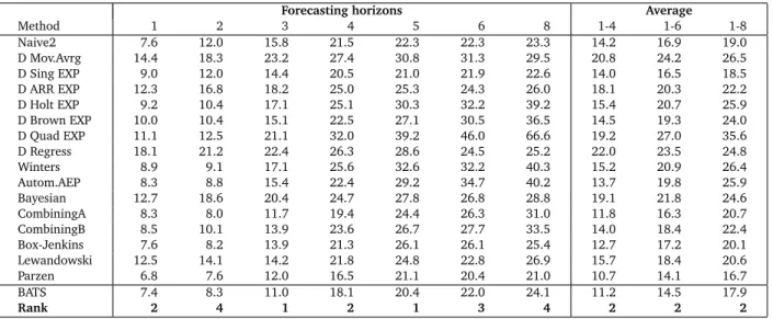
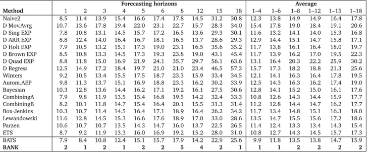
Tables4-6show the out-of-sample MAPE results over a range of forecasting horizons for those methods which take into account any seasonality in the data from the M1 competition for yearly, quarterly and monthly time series respectively. Refer toMakridakis et al.(1982) for details of each method. A ranking obtained by comparing BATS automatic forecasting procedure with the rest of the available methods is also shown. The proposed automatic procedure is ranked first when averaged over all six forecasting horizons for yearly data, ranked second when averaged over all eight forecast horizons for quarterly data and, ranked first when averaged over all eighteen forecast horizons for monthly data. Table7 shows the out-of-sample MAPE for all series along with those results presented in Makridakis et al.
(1982) andHyndman et al.(2002). The BATS procedure ranks first when averaged over the first four and the first six forecast horizons and ranks second for the rest of the averaged forecast horizons up to forecast horizon 18.
Forecasting horizons Average Method 1 2 3 4 5 6 1–4 1–6 Naive2 6.8 9.7 16.6 21.1 23.8 24.8 13.6 17.1 D Mov.Avrg 8.6 10.9 17.7 21.9 24.7 26.0 14.8 18.3 D Sing EXP 6.2 9.1 16.3 21.0 23.6 25.4 13.1 16.9 D ARR EXP 7.8 13.7 17.7 24.4 25.3 29.3 15.9 19.7 D Holt EXP 5.6 7.2 11.9 16.2 19.0 16.5 10.2 12.7 D Brown EXP 6.7 8.2 12.0 16.5 19.8 16.4 10.8 13.3 D Quad EXP 7.0 8.6 11.8 16.0 20.7 17.4 10.9 13.6 D Regress 6.9 7.8 14.9 18.4 20.0 20.6 12.0 14.8 Winters 5.6 7.2 11.9 16.2 19.0 16.5 10.2 12.7 Autom.AEP 7.1 8.8 14.1 17.8 21.8 19.1 11.9 14.8 Bayesian 12.2 12.6 14.9 18.0 20.6 20.6 14.4 16.5 CombiningA 5.7 7.7 12.5 17.4 20.0 17.8 10.8 13.5 CombiningB 6.3 8.3 13.7 17.5 19.7 20.1 11.5 14.3 Box-Jenkins 7.2 10.8 13.7 18.6 23.2 22.3 12.6 16.0 Lewandowski 7.3 8.3 14.7 13.8 16.8 15.1 11.0 12.7 Parzen 7.6 7.7 12.8 16.0 20.5 18.0 11.0 13.8 BATS 5.9 6.7 9.9 13.8 17.1 17.2 9.1 11.8 Rank 4 1 1 1 2 5 1 1
Table 4: Comparison of BATS for 20 yearly time series in the 111 series.
Forecasting horizons Average
Method 1 2 3 4 5 6 8 1-4 1-6 1-8 Naive2 7.6 12.0 15.8 21.5 22.3 22.3 23.3 14.2 16.9 19.0 D Mov.Avrg 14.4 18.3 23.2 27.4 30.8 31.3 29.5 20.8 24.2 26.5 D Sing EXP 9.0 12.0 14.4 20.5 21.0 21.9 22.6 14.0 16.5 18.5 D ARR EXP 12.3 16.8 18.2 25.0 25.3 24.3 26.0 18.1 20.3 22.2 D Holt EXP 9.2 10.4 17.1 25.1 30.3 32.2 39.2 15.4 20.7 25.9 D Brown EXP 10.0 10.4 15.1 22.5 27.1 30.5 36.5 14.5 19.3 24.0 D Quad EXP 11.1 12.5 21.1 32.0 39.2 46.0 66.6 19.2 27.0 35.6 D Regress 18.1 21.2 22.4 26.3 28.6 24.5 25.2 22.0 23.5 24.8 Winters 8.9 9.1 17.1 25.6 32.6 32.2 40.3 15.2 20.9 26.4 Autom.AEP 8.3 8.8 15.4 22.4 29.2 34.7 40.2 13.7 19.8 25.9 Bayesian 12.7 18.6 20.4 24.7 27.8 26.8 28.8 19.1 21.8 24.6 CombiningA 8.3 8.0 11.7 19.4 24.4 26.3 31.0 11.8 16.3 20.7 CombiningB 8.5 10.1 13.9 23.6 26.7 27.7 33.5 14.0 18.4 22.4 Box-Jenkins 7.6 8.2 13.9 21.3 26.1 26.1 25.4 12.7 17.2 20.1 Lewandowski 12.5 14.1 14.2 21.8 24.8 22.8 26.9 15.7 18.4 20.6 Parzen 6.8 7.6 12.0 16.5 21.1 20.4 21.0 10.7 14.1 16.7 BATS 7.4 8.3 11.0 18.1 20.4 22.0 24.1 11.2 14.5 17.9 Rank 2 4 1 2 1 3 4 2 2 2
Table 5: Comparison of BATS for 23 quarterly time series in the 111 series.
Forecasting horizons Average
Method 1 2 3 4 5 6 8 12 15 18 1-4 1-6 1-8 1-12 1-15 1-18 Naive2 9.2 11.7 12.4 11.7 12.6 13.5 16.0 14.5 31.2 30.8 11.3 11.8 13.0 13.7 15.8 17.7 D Mov.Avrg 10.1 12.8 16.0 16.0 18.2 19.4 20.4 15.7 28.3 34.0 13.7 15.4 16.6 16.6 17.8 20.0 D Sing EXP 7.9 10.9 11.7 10.6 11.6 13.2 14.4 13.6 29.3 30.1 10.3 11.0 12.0 12.6 14.5 16.5 D ARR EXP 7.9 10.5 11.5 11.1 11.3 12.7 13.3 13.7 28.6 29.3 10.2 10.8 11.6 12.3 14.2 16.1 D Holt EXP 8.2 11.5 12.3 11.4 12.5 15.2 17.7 16.5 35.6 35.2 10.9 11.8 13.5 14.8 17.2 19.5 D Brown EXP 8.4 11.6 13.0 11.2 13.3 16.4 19.6 19.0 43.1 45.4 11.1 12.3 14.2 16.0 19.5 22.9 D Quad EXP 8.6 12.5 13.8 12.1 16.3 18.7 25.3 29.7 56.1 63.6 11.7 13.7 16.6 20.4 25.7 31.0 D Regress 12.2 14.7 16.0 15.7 16.6 19.9 19.6 23.4 46.5 57.3 14.7 15.9 16.8 18.1 21.4 26.7 Winters 10.3 12.0 12.5 11.8 11.9 14.8 17.5 15.9 33.4 34.5 11.7 12.2 13.6 14.6 16.8 19.1 Autom.AEP 11.2 12.8 13.0 11.9 11.2 13.4 17.6 16.2 30.2 33.9 12.2 12.2 13.4 14.2 16.1 18.4 Bayesian 8.9 10.8 10.9 9.9 10.9 12.8 16.0 16.1 27.5 30.6 10.1 10.7 11.8 12.6 14.5 16.6 CombiningA 8.4 11.1 11.8 10.4 11.1 13.4 15.6 14.2 32.4 33.3 10.4 11.0 12.3 13.1 15.3 17.6 CombiningB 8.6 10.7 10.6 10.8 10.2 11.5 15.6 15.5 31.3 31.4 10.2 10.4 11.7 13.0 15.3 17.4 Box-Jenkins 12.1 11.5 9.9 11.1 11.0 12.5 16.7 16.4 26.2 34.2 11.1 11.3 12.7 13.8 15.6 17.9 Lewandowski 12.6 13.6 14.6 13.5 13.8 16.6 16.2 17.0 33.0 28.6 13.6 14.1 14.4 14.9 17.1 18.9 Parzen 12.7 12.6 9.6 11.7 10.2 11.8 14.3 13.7 22.5 26.5 11.7 11.4 12.1 12.6 13.9 15.4 BATS 8.7 9.0 11.1 10.1 12.7 13.2 15.8 14.2 22.9 25.6 9.7 10.8 12.0 12.8 13.9 15.3 Rank 8 1 5 2 12 6 6 4 2 1 1 3 4 5 1 1
Forecasting horizons Average Method 1 2 3 4 5 6 8 12 15 18 1–4 1–6 1–8 1–12 1–15 1–18 Naive2 8.5 11.4 13.9 15.4 16.6 17.4 17.8 14.5 31.2 30.8 12.3 13.8 14.9 14.9 16.4 17.8 D Mov.Avrg 10.7 13.6 17.8 19.4 22.0 23.1 22.7 15.7 28.3 34.0 15.4 17.8 19.0 18.4 19.1 20.6 D Sing EXP 7.8 10.8 13.1 14.5 15.7 17.2 16.5 13.6 29.3 30.1 11.6 13.2 14.1 14.0 15.3 16.8 D ARR EXP 8.8 12.4 14.0 16.4 16.7 18.1 16.5 13.7 28.6 29.3 12.9 14.4 15.1 14.7 15.8 17.1 D Holt EXP 7.9 10.5 13.2 15.1 17.3 19.0 23.1 16.5 35.6 35.2 11.7 13.8 16.1 16.4 18.0 19.7 D Brown EXP 8.5 10.8 13.3 14.5 17.3 19.3 23.8 19.0 43.1 45.4 11.7 13.9 16.2 17.0 19.5 22.3 D Quad EXP 8.8 11.8 15.0 16.9 21.9 24.1 35.7 29.7 56.1 63.6 13.1 16.4 20.3 22.2 25.9 30.2 D Regress 12.5 14.9 17.2 18.4 19.7 21.0 21.0 23.4 46.5 57.3 15.7 17.3 18.2 18.8 21.3 25.6 Winters 9.2 10.5 13.4 15.5 17.5 18.7 23.3 15.9 33.4 34.5 12.1 14.1 16.3 16.4 17.8 19.5 Autom.AEP 9.8 11.3 13.7 15.1 16.9 18.8 23.3 16.2 30.2 33.9 12.5 14.3 16.3 16.2 17.4 19.0 Bayesian 10.3 12.8 13.6 14.4 16.2 17.1 19.2 16.1 27.5 30.6 12.8 14.1 15.2 15.0 16.1 17.6 CombiningA 7.9 9.8 11.9 13.5 15.4 16.8 19.5 14.2 32.4 33.3 10.8 12.6 14.3 14.4 15.9 17.7 CombiningB 8.2 10.1 11.8 14.7 15.4 16.4 20.1 15.5 31.3 31.4 11.2 12.8 14.4 14.7 16.2 17.7 Box-Jenkins 10.3 10.7 11.4 14.5 16.4 17.1 18.9 16.4 26.2 34.2 11.7 13.4 14.8 15.1 16.3 18.0 Lewandowski 11.6 12.8 14.5 15.3 16.6 17.6 18.9 17.0 33.0 28.6 13.5 14.7 15.5 15.6 17.2 18.6 Parzen 10.6 10.7 10.7 13.5 14.3 14.7 16.0 13.7 22.5 26.5 11.4 12.4 13.3 13.4 14.3 15.4 ETS 8.7 9.2 11.9 13.3 16.0 16.9 19.2 15.2 28.0 31.0 10.8 12.7 14.3 14.5 15.7 17.3 BATS 7.9 8.4 10.8 12.4 15.1 15.7 17.9 14.2 22.9 25.6 9.9 11.8 13.5 13.8 14.7 15.9 RANK 2 1 2 1 2 2 5 4 2 1 1 1 2 2 2 2
Table 7: Comparison of BATS automatic forecasting procedure for all 111 series.
3.2 Application to 1001 series
The automatic forecasting procedure was then applied to the 1001 series. Table8shows the out-of-sample MAPE comparison between the BATS automatic procedure and the results obtained from those methods presented in Makridakis et al. (1982) and Hyndman et al.
(2002). Only those methods which take into account any seasonality in the data are presented in the table. As with the 111 series, a ranking is provided for comparison. In comparison with the rest of the methods, the BATS method is ranked second when averaged over the first four, the first six and the first eight forecast horizons. When averaged over the first twelve and fifteen, it is ranked fourth, and ranked fifth when averaged over the first eighteen.
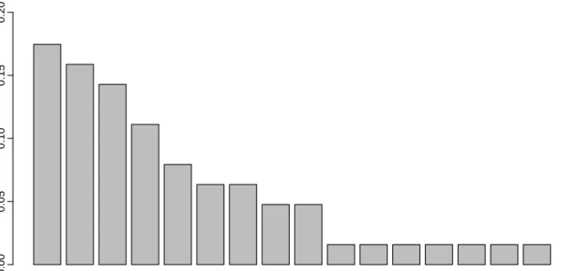
Table 9 shows the percentage of each BATS model combination selected for the 1001 series. 54.4% of the chosen models are non-seasonal models, and out of these, N(simple exponential smoothing),T(Holt’s method) andBT(Holt’s method with an integrated Box-Cox transformation) are the most commonly chosen models. Non-trended seasonal models, that is SandBS are the most commonly chosen seasonal models. Models with an integrated Box-Cox transformation have been chosen 43.5% of the time, and approximately 96% of the values for ω selected by using the RMSE criterion were between 0 and 0.3. Models with residual ARMA adjustment have been selected 6.3% of the time, and as shown by the
relative frequency diagram in Figure 1, pure AR and MA models are the most frequently selected.
Forecasting horizons Average of forecasting horizons Method 1 2 3 4 5 6 8 12 15 18 1–4 1–6 1–8 1–12 1–15 1–18 Naive2 9.1 11.3 13.3 14.6 18.4 19.9 19.1 17.1 21.9 26.3 12.1 14.4 15.2 15.7 16.4 17.4 D Mov.Avrg 11.5 14.9 17.0 17.8 21.5 22.3 20.6 17.8 23.2 29.4 15.3 17.5 18.1 18.1 18.6 19.6 D Sing EXP 8.6 11.6 13.2 14.1 17.7 19.5 17.9 16.9 21.1 26.1 11.9 14.1 14.8 15.3 16.0 16.9 D ARR EXP 9.4 13.5 14.0 15.3 18.1 20.2 18.0 17.1 21.4 26.0 13.1 15.1 15.6 15.9 16.5 17.4 D Holt EXP 8.7 11.0 13.3 15.2 19.1 21.6 24.8 23.9 33.7 48.3 12.1 14.8 16.7 18.4 20.2 22.9 D Brown EXP 8.7 10.9 13.8 15.0 18.7 21.1 24.5 23.1 30.8 43.7 12.1 14.7 16.6 18.0 19.6 21.9 D Quad EXP 9.8 12.7 16.6 18.8 25.7 31.0 45.1 40.7 64.4 108.3 14.5 19.1 23.7 26.9 31.2 38.5 D Regress 15.5 16.9 19.1 18.3 21.9 23.0 24.2 29.7 49.1 70.7 17.4 19.1 20.0 22.6 25.5 29.8 Winters 8.7 10.9 13.2 14.9 19.0 21.5 24.3 23.0 32.8 47.0 11.9 14.7 16.5 18.1 19.8 22.4 Autom.AEP 9.1 11.9 13.4 13.7 17.9 20.3 20.3 19.3 24.8 28.8 12.0 14.4 15.5 16.3 17.5 18.8 Bayesian 11.2 12.8 14.5 16.2 19.8 22.3 22.6 18.9 23.5 28.3 13.7 16.1 17.2 17.6 18.3 19.3 CombiningA 8.1 10.4 12.1 13.3 16.7 19.2 19.7 18.6 24.2 30.8 11.0 13.3 14.5 15.4 16.5 17.9 CombiningB 8.5 11.1 12.8 13.8 17.6 19.2 18.9 18.4 23.3 30.3 11.6 13.8 14.8 15.6 16.5 17.8 ETS 9.0 10.8 12.8 13.4 17.4 19.3 19.5 17.2 23.4 29.0 11.5 13.8 14.7 15.4 16.4 17.6 BATS 8.6 11.2 12.6 13.3 16.8 18.7 19.2 17.1 21.5 26.9 11.4 13.5 14.7 15.5 16.5 17.7 Rank 3 7 2 1 2 1 5 2 3 4 2 2 2 4 4 5
Table 8: Comparison of BATS automatic forecasting procedure for 1001 series.
Seasonal Non-seasonal
Linear Non-linear Linear Non-linear
Model Percentage Model Percentage Model Percentage Model Percentage
S 17.6 BS 16.0 N 13.7 B 4.6
TS 2.8 BTS 4.7 T 9.6 BT 10.0
TdS 1.1 BTdS 2.2 Td 7.3 BTd 4.2
AS 0.9 BAS 0.3 A 2.0 BA 0.8
ATS 0.0 BATS 0.0 AT 0.9 BAT 0.5
ATdS 0.0 BATdS 0.1 ATd 0.7 BATd 0.1
Total 22.4 Total 23.3 Total 34.2 Total 20.2
(0,1) (0,2) (2,0) (3,0) (0,3) (5,0) (1,1) (0,4) (1,0) (0,5) (4,0) (4,1) (3,2) (2,3) (1,2) (3,1) ARMA order Relative frequency 0.00 0.05 0.10 0.15 0.20
Figure 1: Relative frequency diagram for ARMA orders{p,q}selected for 1001 series.
3.3 Application to 3003 series
Based on the results obtained for the 111 and the 1001 series, using the RMSE as the estimation criterion and the residual ARMA fitting approach (ii), the BATS algorithm was fitted to the 3003 series in the M3-competition. The out-of-sample performance was compared with those methods inMakridakis & Hibon(2000) andHyndman et al.(2002). In comparing the results, thesymmetric mean absolute percentage error(sMAPE) was used, as it enables comparisons with published M3 results. However some authors such asHyndman & Koehler (2006) recommend against the use of sMAPE. Although several variations of sMAPE appear in forecasting literature (Armstrong 1985,Makridakis 1993,Chen & Yang 2004,Andrawis & Atiya 2009), these variations generate the same results, as all the obser-vations in the 3003 series are positive, andMakridakis & Hibon(2000) lets any negative forecasts equal to zero.
The out-of-sample results obtained for quarterly, monthly, yearly, other and all 3003 series are shown in Tables10-14respectively, along with the results for ETS method and those methods from the M3-competition.
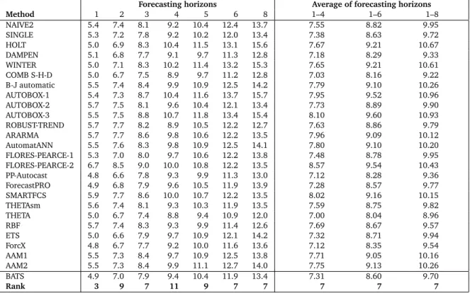
Forecasting horizons Average of forecasting horizons Method 1 2 3 4 5 6 8 1–4 1–6 1–8 NAIVE2 5.4 7.4 8.1 9.2 10.4 12.4 13.7 7.55 8.82 9.95 SINGLE 5.3 7.2 7.8 9.2 10.2 12.0 13.4 7.38 8.63 9.72 HOLT 5.0 6.9 8.3 10.4 11.5 13.1 15.6 7.67 9.21 10.67 DAMPEN 5.1 6.8 7.7 9.1 9.7 11.3 12.8 7.18 8.29 9.33 WINTER 5.0 7.1 8.3 10.2 11.4 13.2 15.3 7.65 9.21 10.61 COMB S-H-D 5.0 6.7 7.5 8.9 9.7 11.2 12.8 7.03 8.16 9.22 B-J automatic 5.5 7.4 8.4 9.9 10.9 12.5 14.2 7.79 9.10 10.26 AUTOBOX-1 5.4 7.3 8.7 10.4 11.6 13.7 15.7 7.95 9.52 10.96 AUTOBOX-2 5.7 7.5 8.1 9.6 10.4 12.1 13.4 7.73 8.89 9.90 AUTOBOX-3 5.5 7.5 8.8 10.7 11.8 13.4 15.4 8.10 9.60 10.93 ROBUST-TREND 5.7 7.7 8.2 8.9 10.5 12.2 12.7 7.63 8.86 9.79 ARARMA 5.7 7.7 8.6 9.8 10.6 12.2 13.5 7.96 9.09 10.12 AutomatANN 5.5 7.6 8.3 9.8 10.9 12.5 14.1 7.80 9.10 10.20 FLORES-PEARCE-1 5.3 7.0 8.0 9.7 10.6 12.2 13.8 7.48 8.78 9.95 FLORES-PEARCE-2 6.7 8.5 9.0 10.0 10.8 12.2 13.5 8.57 9.54 10.43 PP-Autocast 4.8 6.6 7.8 9.3 9.9 11.3 13.0 7.12 8.28 9.36 ForecastPRO 4.9 6.8 7.9 9.6 10.5 11.9 13.9 7.28 8.57 9.77 SMARTFCS 5.9 7.7 8.6 10.0 10.7 12.2 13.5 8.02 9.16 10.15 THETAsm 5.6 7.4 8.1 9.3 10.3 11.9 13.5 7.59 8.75 9.82 THETA 5.0 6.7 7.4 8.8 9.4 10.9 12.0 7.00 8.04 8.96 RBF 5.7 7.4 8.3 9.3 9.9 11.4 12.6 7.69 8.67 9.57 ETS 5.0 6.6 7.9 9.7 10.9 12.1 14.2 7.32 8.71 9.94 ForcX 4.8 6.7 7.7 9.2 10.0 11.6 13.6 7.12 8.35 9.54 AAM1 5.5 7.3 8.4 9.7 10.9 12.5 13.8 7.71 9.05 10.16 AAM2 5.5 7.3 8.4 9.9 11.1 12.7 14.0 7.75 9.13 10.26 BATS 4.9 7.0 7.9 9.4 10.4 11.9 13.4 7.31 8.60 9.70 Rank 3 9 7 11 9 7 7 7 7 7
Table 10: Average sMAPE across different forecast horizons: 756 quarterly series.
Forecasting horizons Average of forecasting horizons Method 1 2 3 4 5 6 8 12 15 18 1–4 1–6 1–8 1–12 1–15 1–18 NAIVE2 15.0 13.5 15.7 17.0 14.9 14.4 15.6 16.0 19.3 20.7 15.30 15.08 15.26 15.55 16.16 16.89 SINGLE 13.0 12.1 14.0 15.1 13.5 12.8 13.8 14.5 18.3 19.4 13.53 13.39 13.56 13.81 14.49 15.30 HOLT 12.2 11.6 13.4 14.6 13.6 12.9 13.7 14.8 18.8 20.2 12.95 13.05 13.29 13.74 14.49 15.34 DAMPEN 11.9 11.4 13.0 14.2 12.9 12.3 13.0 13.9 17.5 18.9 12.63 12.63 12.81 13.08 13.75 14.58 WINTER 12.5 11.7 13.7 14.7 13.6 13.0 14.1 14.6 18.9 20.2 13.17 13.23 13.48 13.86 14.60 15.42 COMB S-H-D 12.3 11.5 13.2 14.3 12.9 12.2 13.0 13.6 17.3 18.3 12.83 12.74 12.88 13.09 13.73 14.47 B-J automatic 12.3 11.7 12.8 14.3 12.7 12.3 13.0 14.1 17.8 19.3 12.78 12.70 12.86 13.19 13.95 14.80 AUTOBOX-1 13.0 12.2 13.0 14.8 14.1 13.1 14.3 15.4 19.1 20.4 13.27 13.37 13.67 14.07 14.91 15.81 AUTOBOX-2 13.1 12.1 13.5 15.3 13.3 13.5 13.9 15.2 18.2 19.9 13.51 13.47 13.72 14.14 14.84 15.67 AUTOBOX-3 12.3 12.3 13.0 14.4 14.6 13.9 14.8 16.1 19.2 21.2 12.99 13.41 13.84 14.39 15.17 16.16 ROBUST-TREND 15.3 13.8 15.5 17.0 15.3 15.3 17.4 17.5 22.2 24.3 15.39 15.37 15.85 16.55 17.45 18.38 ARARMA 13.1 12.4 13.4 14.9 13.7 13.9 15.0 15.2 18.5 20.3 13.42 13.55 13.96 14.39 15.06 15.83 AutomatANN 11.6 11.6 12.0 14.1 12.2 13.6 13.8 14.6 17.3 19.6 12.31 12.51 12.89 13.41 14.12 14.91 FLORES-PEARCE-1 12.4 12.3 14.2 16.1 14.6 13.9 14.6 14.4 19.1 20.8 13.74 13.92 14.21 14.28 15.01 15.95 FLORES-PEARCE-2 12.6 12.1 13.7 14.7 13.2 12.8 13.4 14.4 18.2 19.9 13.26 13.18 13.31 13.52 14.30 15.17 PP-Autocast 12.7 11.7 13.3 14.3 13.2 13.1 14.0 14.3 17.7 19.6 13.02 13.05 13.33 13.70 14.34 15.13 ForecastPRO 11.5 10.7 11.7 12.9 11.8 12.0 12.6 13.2 16.4 18.3 11.72 11.78 12.02 12.43 13.07 13.85 SMARTFCS 11.6 11.2 12.2 13.6 13.1 13.4 13.5 14.9 18.0 19.4 12.16 12.53 12.85 13.49 14.20 15.01 THETAsm 12.9 12.2 13.6 14.3 14.1 14.1 14.0 14.2 17.6 19.1 13.24 13.52 13.81 14.03 14.54 15.24 THETA 11.2 10.7 11.8 12.4 12.2 12.2 12.7 13.2 16.2 18.2 11.54 11.75 12.09 12.48 13.09 13.83 RBF 13.7 12.3 13.7 14.3 12.3 12.5 13.5 14.1 17.3 17.8 13.49 13.14 13.36 13.64 14.19 14.76 ForcX 11.6 11.2 12.6 14.0 12.4 12.0 12.8 13.9 17.8 18.7 12.32 12.28 12.44 12.81 13.58 14.44 ETS 11.5 10.6 12.3 13.4 12.3 12.3 13.2 14.1 17.6 18.9 11.93 12.05 12.43 12.96 13.64 14.45 AAM1 12.0 12.3 12.7 14.1 14.0 13.7 14.3 14.9 18.0 20.4 12.80 13.16 13.59 14.03 14.77 15.67 AAM2 12.3 12.4 12.9 14.4 14.3 13.9 14.5 15.1 18.4 20.7 13.03 13.40 13.83 14.23 15.00 15.92 BATS 11.9 10.9 12.6 13.3 12.2 12.2 13.4 13.8 17.2 18.9 12.20 12.20 12.49 12.99 13.68 14.47 Rank 7 4 6 3 2 3 8 4 3 6 5 4 5 5 5 5
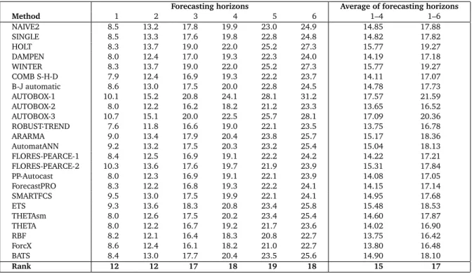
Forecasting horizons Average of forecasting horizons Method 1 2 3 4 5 6 1–4 1–6 NAIVE2 8.5 13.2 17.8 19.9 23.0 24.9 14.85 17.88 SINGLE 8.5 13.3 17.6 19.8 22.8 24.8 14.82 17.82 HOLT 8.3 13.7 19.0 22.0 25.2 27.3 15.77 19.27 DAMPEN 8.0 12.4 17.0 19.3 22.3 24.0 14.19 17.18 WINTER 8.3 13.7 19.0 22.0 25.2 27.3 15.77 19.27 COMB S-H-D 7.9 12.4 16.9 19.3 22.2 23.7 14.11 17.07 B-J automatic 8.6 13.0 17.5 20.0 22.8 24.5 14.78 17.73 AUTOBOX-1 10.1 15.2 20.8 24.1 28.1 31.2 17.57 21.59 AUTOBOX-2 8.0 12.2 16.2 18.2 21.2 23.3 13.65 16.52 AUTOBOX-3 10.7 15.1 20.0 22.5 25.7 28.1 17.09 20.36 ROBUST-TREND 7.6 11.8 16.6 19.0 22.1 23.5 13.75 16.78 ARARMA 9.0 13.4 17.9 20.4 23.8 25.7 15.17 18.36 AutomatANN 9.2 13.2 17.5 20.3 23.2 25.4 15.04 18.13 FLORES-PEARCE-1 8.4 12.5 16.9 19.1 22.2 24.2 14.22 17.21 FLORES-PEARCE-2 10.3 13.6 17.6 19.7 21.9 23.9 15.31 17.84 PP-Autocast 8.0 12.3 16.9 19.1 22.1 23.9 14.08 17.05 ForecastPRO 8.3 12.2 16.8 19.3 22.2 24.1 14.15 17.14 SMARTFCS 9.5 13.0 17.5 19.9 22.1 24.1 14.95 17.68 ETS 9.3 13.6 18.3 20.8 23.4 25.8 15.48 18.53 THETAsm 8.0 12.6 17.5 20.2 23.4 25.4 14.60 17.87 THETA 8.0 12.2 16.7 19.2 21.7 23.6 14.02 16.90 RBF 8.2 12.1 16.4 18.3 20.8 22.7 13.75 16.42 ForcX 8.6 12.4 16.1 18.2 21.0 22.7 13.80 16.48 BATS 8.4 13.0 17.7 20.4 23.5 25.6 14.90 18.10 Rank 12 12 17 18 19 18 15 17
Table 12: Average sMAPE across different forecast horizons: 645 yearly series.
Forecasting horizons Average of forecasting horizons
Method 1 2 3 4 5 6 8 1–4 1–6 1–8 NAIVE2 2.2 3.6 5.4 6.3 7.8 7.6 9.2 4.38 5.49 6.30 SINGLE 2.1 3.6 5.4 6.3 7.8 7.6 9.2 4.36 5.48 6.29 HOLT 1.9 2.9 3.9 4.7 5.8 5.6 7.2 3.32 4.13 4.81 DAMPEN 1.8 2.7 3.9 4.7 5.8 5.4 6.6 3.28 4.06 4.61 WINTER 1.9 2.9 3.9 4.7 5.8 5.6 7.2 3.32 4.13 4.81 COMB S-H-D 1.8 2.8 4.1 4.7 5.8 5.3 6.2 3.36 4.09 4.56 B-J automatic 1.8 3.0 4.5 4.9 6.1 6.1 7.5 3.52 4.38 5.06 AUTOBOX-1 2.4 3.3 4.4 4.9 5.8 5.4 6.9 3.76 4.38 4.93 AUTOBOX-2 1.6 2.9 4.0 4.3 5.3 5.1 6.4 3.19 3.86 4.41 AUTOBOX-3 1.9 3.2 4.1 4.4 5.5 5.5 7.0 3.39 4.09 4.71 ROBUST-TREND 1.9 2.8 3.9 4.7 5.7 5.4 6.4 3.32 4.07 4.58 ARARMA 1.7 2.7 4.0 4.4 5.5 5.1 6.0 3.17 3.87 4.38 AutomatANN 1.7 2.9 4.0 4.5 5.7 5.7 7.4 3.26 4.07 4.80 FLORES-PEARCE-1 2.1 3.2 4.3 5.2 6.2 5.8 7.3 3.71 4.47 5.09 FLORES-PEARCE-2 2.3 2.9 4.3 5.1 6.2 5.7 6.5 3.67 4.43 4.89 PP-Autocast 1.8 2.7 4.0 4.7 5.8 5.4 6.6 3.29 4.07 4.62 ForecastPRO 1.9 3.0 4.0 4.4 5.4 5.4 6.7 3.31 4.00 4.60 SMARTFCS 2.5 3.3 4.3 4.7 5.8 5.5 6.7 3.68 4.33 4.86 ETS 2.0 3.0 4.0 4.4 5.4 5.1 6.3 3.37 3.99 4.51 THETAsm 2.3 3.2 4.3 4.8 6.0 5.6 6.9 3.66 4.37 4.93 THETA 1.8 2.7 3.8 4.5 5.6 5.2 6.1 3.20 3.93 4.41 RBF 2.7 3.8 5.2 5.8 6.9 6.3 7.3 4.38 5.12 5.60 ForcX 2.1 3.1 4.1 4.4 5.6 5.4 6.5 3.42 4.10 4.64 BATS 1.7 2.8 3.9 4.2 5.1 5.0 6.3 3.17 3.78 4.32 Rank 2 5 2 1 1 1 4 1 1 1
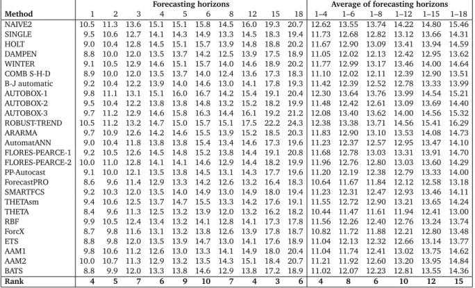
Forecasting horizons Average of forecasting horizons Method 1 2 3 4 5 6 8 12 15 18 1–4 1–6 1–8 1–12 1–15 1–18 NAIVE2 10.5 11.3 13.6 15.1 15.1 15.8 14.5 16.0 19.3 20.7 12.62 13.55 13.74 14.22 14.80 15.46 SINGLE 9.5 10.6 12.7 14.1 14.3 14.9 13.3 14.5 18.3 19.4 11.73 12.68 12.82 13.12 13.66 14.31 HOLT 9.0 10.4 12.8 14.5 15.1 15.7 13.9 14.8 18.8 20.2 11.67 12.90 13.09 13.41 13.94 14.59 DAMPEN 8.8 10.0 12.0 13.5 13.7 14.2 12.5 13.9 17.5 18.9 11.05 12.02 12.13 12.42 12.95 13.62 WINTER 9.1 10.5 12.9 14.6 15.1 15.7 14.0 14.6 18.9 20.2 11.77 12.99 13.17 13.46 14.00 14.64 COMB S-H-D 8.9 10.0 12.0 13.5 13.7 14.0 12.4 13.6 17.3 18.3 11.10 12.02 12.11 12.39 12.90 13.51 B-J automatic 9.2 10.4 12.2 13.9 14.0 14.6 13.0 14.1 17.8 19.3 11.42 12.39 12.52 12.78 13.33 13.99 AUTOBOX-1 9.8 11.1 13.1 15.1 16.0 16.7 14.2 15.4 19.1 20.4 12.30 13.64 13.76 13.99 14.54 15.21 AUTOBOX-2 9.5 10.4 12.2 13.8 13.8 14.8 13.2 15.2 18.2 19.9 11.48 12.42 12.61 13.09 13.69 14.40 AUTOBOX-3 9.7 11.2 12.9 14.6 15.8 16.3 14.4 16.1 19.2 21.2 12.08 13.40 13.62 14.00 14.56 15.32 ROBUST-TREND 10.5 11.2 13.2 14.7 15.0 15.7 15.1 17.5 22.2 24.3 12.38 13.38 13.71 14.56 15.41 16.29 ARARMA 9.7 10.9 12.6 14.2 14.6 15.5 13.9 15.2 18.5 20.3 11.83 12.90 13.10 13.53 14.08 14.73 AutomatANN 9.0 10.4 11.8 13.8 13.8 15.4 13.4 14.6 17.3 19.6 11.23 12.37 12.57 12.95 13.47 14.10 FLORES-PEARCE-1 9.2 10.5 12.6 14.5 14.8 15.2 13.8 14.4 19.1 20.8 11.68 12.78 13.03 13.31 13.91 14.70 FLORES-PEARCE-2 10.0 11.0 12.8 14.1 14.1 14.6 12.9 14.4 18.2 19.9 11.96 12.76 12.80 13.03 13.60 14.29 PP-Autocast 9.1 10.0 12.1 13.5 13.8 14.5 13.1 14.3 17.7 19.6 11.20 12.19 12.38 12.79 13.33 14.00 ForecastPRO 8.6 9.6 11.4 12.9 13.3 14.2 12.6 13.2 16.4 18.3 10.64 11.67 11.84 12.12 12.58 13.18 SMARTFCS 9.2 10.3 12.0 13.5 14.0 14.9 13.0 14.9 18.0 19.4 11.23 12.31 12.47 12.93 13.46 14.11 THETAsm 9.4 10.6 12.5 13.7 14.7 15.5 13.3 14.2 17.6 19.1 11.55 12.72 12.90 13.21 13.65 14.24 THETA 8.4 9.6 11.3 12.5 13.2 13.9 12.0 13.2 16.2 18.2 10.44 11.47 11.61 11.94 12.41 13.00 RBF 9.9 10.5 12.4 13.4 13.2 14.1 12.8 14.1 17.3 17.8 11.56 12.26 12.40 12.76 13.24 13.74 ForcX 8.7 9.8 11.6 13.1 13.2 13.8 12.6 13.9 17.8 18.7 10.82 11.72 11.88 12.21 12.80 13.48 ETS 8.8 9.8 12.0 13.5 13.9 14.7 13.0 14.1 17.6 18.9 11.04 12.13 12.32 12.66 13.14 13.77 AAM1 9.8 10.6 11.2 12.6 13.0 13.3 14.1 14.9 18.0 20.4 11.04 11.74 12.41 13.02 13.75 14.62 AAM2 10.0 10.7 11.3 12.9 13.2 13.5 14.3 15.1 18.4 20.7 11.21 11.92 12.60 13.20 13.95 14.84 BATS 8.8 9.9 12.0 13.3 13.8 14.6 12.9 13.8 17.2 18.9 11.02 12.07 12.23 12.81 13.55 14.36 Rank 4 5 7 6 9 10 7 4 3 6 4 8 6 10 12 15
Table 14: Average sMAPE across different forecast horizons: all 3003 series.
These results demonstrate that the proposed BATS automatic procedure is comparable with the rest of the methods. It performs very well on theotherseries, being ranked first for all averaged forecast horizons.
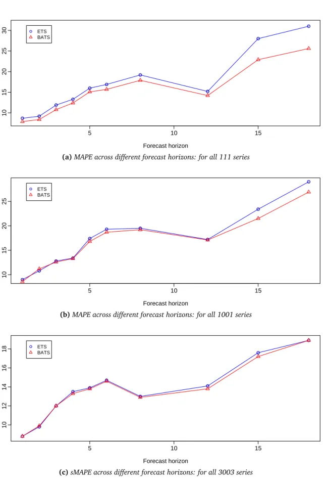
As with the results obtained for all 111 and all 1001 series, the results obtained for all 3003 series show that the proposed BATS algorithm outperformed the ETS method when averaged over the first four and the first six forecast horizons (See Tables 7, 8and 14). Figure2
provides a graphical illustration of the comparison between BATS and ETS forecasting algorithms for all 111, 1001 and 3003 series, showing that the BATS automatic procedure offers competitive results to traditional exponential smoothing models.
● ● ● ● ● ● ● ● ● ● 5 10 15 10 15 20 25 30 Forecast horizon MAPE ● ● ● ● ● ● ● ● ● ● ● ETS BATS
(a)MAPE across different forecast horizons: for all 111 series
● ● ● ● ● ● ● ● ● ● 5 10 15 10 15 20 25 Forecast horizon MAPE ● ● ● ● ● ● ● ● ● ● ● ETS BATS
(b)MAPE across different forecast horizons: for all 1001 series
● ● ● ● ● ● ● ● ● ● 5 10 15 10 12 14 16 18 Forecast horizon sMAPE ● ● ● ● ● ● ● ● ● ● ● ETS BATS
(c)sMAPE across different forecast horizons: for all 3003 series
Figure 2: The out-of-sample performance across different forecast horizons, comparing BATS with ETS (a) for all 111 series (b) for all 1001 series (c) for all 3003 series.
4
Application to multiple seasonal data
In this section, applications of the automatic BATS exponential smoothing algorithm to multiple seasonal time series are considered. In the existing forecasting literature, automatic modeling procedures for multiple seasonal time series are not available. As with the non-seasonal and single non-seasonal series, RMSE as the estimation criterion and approach (ii) as the ARMA selection procedure were used.
Figure3shows a time series of the number of calls at a large US bank, starting from March 3 2003. The data are half hourly and consist of 1500 observations. The figure depicts a daily seasonal pattern with frequency m1 =28 and a weekly seasonal pattern with frequency
m2 = 28∗5 = 140. The proposed BATS automatic procedure was applied to this data
Half−hours Number of calls 0 500 1000 1500 500 1000 1500 2000
Figure 3: Half hourly call center data provided by a large bank in US, starting from March 3 2003
set and the model BATS(2, 2, 28, 140) without a Box-Cox transformation was selected by the automated algorithm, with parameter estimates of αˆ = −0.0116,βˆ = 0.0048,γˆ1 = 0.0557,γˆ2=0.1778,φˆ=0.8558,ϕˆ1=1.2341,ϕˆ2=−0.3245,θˆ1=−0.7458,θˆ2 =0.2542. The trend, seasonal and irregular components obtained by the selected BATS model are shown in Figure4. The vertical bars at the right side of each sub-plot are of equal heights but plotted on different scales, providing a comparison of the size of each component. Small estimated values forαandβ indicate that the level and the slope of the trend component
is almost deterministic implying a global trend, and the estimated value of 0.8558 for φ implies a damping effect. In forecasting, this will dampen the trend component as the length of the forecast horizon increases. It is seen in Figure4that this trend component is relatively small compared to the seasonal components. Likewise, the time series plot itself (shown in Figure 3) depicts a small, stable trend component. The estimated values ofγ1 andγ2, together with Figure 4indicate that the weekly seasonal component is considerably variable over time while the daily seasonal component stays relatively stable. The model implies that the irregular component of the series is correlated and can be described by an ARMA(2, 2) process. 500 1500 data 1100 1250 trend −800 0 400 daily −200 0 200 weekly −300 0 200 remainder Half−hours 1 500 1000 1500
Figure 4: Decomposition obtained for the call center data from the BATS automatic procedure
Figure 5 presents the analytical point predictions and 95% interval predictions up to a day ahead together with the actual values. It is seen that the point predictions follow the observed series closely, with the prediction intervals containing almost all the observed values.
The second application involves a time series of electricity demand in England and Wales beginning June 2000, recorded at half hourly intervals. A double seasonal pattern can be clearly seen in the time series plot shown in Figure6. The within-day seasonal pattern has a
Half−hours Number of calls 1500 1505 1510 1515 1520 1525 400 600 800 1000 1200 1400 1600 ● ● ● ● ● ● ● ● ● ● ● ● ● ● ● ● ● ● ● ● ● ● ● ● ● ● ● ● ● Actual Point predictions Interval predictions
Figure 5: A comparison of the out-of-sample call center forecasts with the actual values up to 28 half hours ahead
duration of m1=48 half-hour periods and the within-week seasonal pattern has a duration of m2=336 half-hour periods. The data consists of 5 weeks of observations, that is 1680 values. For such electricity demand series,Taylor(2003,2008) points out the importance of short term and very short term forecasts for the real-time scheduling of electricity generation.
Half−hours Electricity demand (MW) 0 500 1000 1500 20000 25000 30000 35000
For this series, the automatic BATS forecasting procedure led to the selection of BATS(4, 0, 48, 336) model with no Box-Cox transformation. The estimated parameters are as follows. αˆ=0.0089,βˆ=0,γˆ1=0.1059,γˆ2=0.0180,φˆ=0.9998,ϕˆ1=0.9234,ϕˆ2= 0.1399,ϕˆ3=−0.1252,ϕˆ4 =−0.0278. The estimated values of 0.0089 forα and 0 forβ suggest a global trend component with a purely deterministic growth rate. The damping effect of the trend component is negligible as implied by the estimated value forφ which is almost 1. Figure7shows the trend, seasonal and irregular components obtained by the selected model. It indicates that the trend component of the series is relatively small and that the weekly seasonal component does not have much variation over time. The irregular component is correlated and is modeled by an ARMA(4, 0) process. Figure8presents the analytical point predictions and 95% interval predictions up to 28 steps ahead together with the actual values. As with the call center application, it is seen that the point predictions follow the observed series closely, and that the narrow prediction intervals contain virtually all the out-of-sample observations.
20000 35000 data 29900 30300 trend −8000 0 6000 daily −8000 0 weekly −1000 500 remainder Half−hours 1 500 1000 1500
Figure 7: Decomposition obtained for the electricity demand data from the BATS automatic procedure
Half−hours Electricity demand (MW) 1680 1685 1690 1695 1700 1705 25000 30000 35000 ● ● ● ● ● ● ● ● ● ● ● ● ● ● ● ● ● ● ● ● ● ● ● ● ● ● ● ● ● Actual Point predictions Interval predictions (a)
Figure 8: A comparison of the out-of-sample electricity demand forecasts with the actual values up to 28 half hours ahead
5
Conclusion
In this paper, a new automatic exponential smoothing framework is introduced, which is complete with straightforward initialization and estimation procedures including likelihood evaluation, and the computation of point forecasts and prediction intervals. The new algorithm provides an alternative to existing automatic forecasting practices; but provides the option of modeling time series with multiple seasonal patterns, which cannot be handled using any of the existing automatic forecasting procedures.
The proposed BATS automatic procedure is shown to perform well in applications to the 111 and the 1001 series from the M competition and to the 3003 series from the M3 competition, and is comparable with the best methods of these competitions. The out-of-sample forecast accuracy results obtained for all 111, 1001 and 3003 series (presented in Tables 7,8and
14respectively) showed that the BATS automatic algorithm outperformed the traditional exponential smoothing framework when averaged over the first four and the first six forecast horizons. Two applications involving call center data and electricity demand data were used to illustrate the competency of the BATS automatic approach for forecasting multiple seasonal time series. The methods used in this paper for the implementation of the BATS
automatic procedure will be available in theforecastpackage for R (Hyndman & Khandakar 2008).
Acknowledgement
I thank Rob Hyndman, Ralph Snyder and Peter Toscas for providing valuable comments which improved this paper. I also thank Michèle Hibon for providing the out-of-sample results for the M competition and the M3 competition, and James Taylor for providing the electricity demand data.
References
Akram, M., Hyndman, R. & Ord, J. (2009), ‘Exponential smoothing and non-negative data’,
Australian & New Zealand Journal of Statistics51(4), 415–432.
Andrawis, R. & Atiya, A. (2009), ‘A new Bayesian formulation for Holt’s exponential smooth-ing’,Journal of Forecasting28(3), 218–234.
Armstrong, J. S. (1985),Long-range forecasting: from crystal ball to computer, Wiley.
Billah, B., Hyndman, R. J. & Koehler, A. B. (2005), ‘Empirical information criteria for time series forecasting model selection’, Journal of Statistical Computation and Simulation
75, 831–840.
Brown, R. G. (1959),Statistical forecasting for inventory control, McGraw-Hill, New York. Burnham, K. P. & Anderson, D. R. (2002),Model selection and multimodel inference: a practical
information-theoretic approach, 2nd edn, Springer-Verlag.
Chen, Z. & Yang, Y. (2004), ‘Assessing forecast accuracy measures’,Preprint Seriespp. 2004– 10.
De Livera, A. & Hyndman, R. (2009), Forecasting time series with complex seasonal patterns using exponential smoothing, Working paper 15/09, Department of Econometrics & Business Statistics, Monash University.
Gardner, Jr, E. S. (1985), ‘Exponential smoothing: The state of the art’,Journal of Forecasting
4, 1–28.
Gardner, Jr, E. S. & McKenzie, E. (1985), ‘Forecasting trends in time series’,31(10), 1237– 1246.
Geriner, P. & Ord, J. (1991), ‘Automatic forecasting using explanatory variables: A compara-tive study’,International Journal of Forecasting7(2), 127–140.
Holt, C. C. (1957), Forecasting trends and seasonals by exponentially weighted averages, O.N.R. Memorandum 52/1957, Carnegie Institute of Technology.
Hyndman, R. J., Akram, M. & Archibald, B. C. (2007), ‘The admissible parameter space for exponential smoothing models’,Annals of the Institute of Statistical Mathematics60, 407– 426.
Hyndman, R. J. & Koehler, A. B. (2006), ‘Another look at measures of forecast accuracy’,
International Journal of Forecasting22, 679–688.
Hyndman, R. J., Koehler, A. B., Ord, J. K. & Snyder, R. D. (2005), ‘Prediction intervals for exponential smoothing using two new classes of state space models’,Journal of Forecasting
24, 17–37.
Hyndman, R. J., Koehler, A. B., Ord, J. K. & Snyder, R. D. (2008),Forecasting with exponential smoothing: the state space approach, Springer-Verlag, Berlin.
URL:www.exponentialsmoothing.net
Hyndman, R. J., Koehler, A. B., Snyder, R. D. & Grose, S. (2002), ‘A state space framework for automatic forecasting using exponential smoothing methods’,International Journal of Forecasting18(3), 439–454.
Hyndman, R. & Khandakar, Y. (2008), ‘Automatic time series forecasting: The forecast package for R’,Journal of Statistical Software26(3).
Makridakis, S. (1993), ‘Accuracy measures: theoretical and practical concerns’,International Journal of Forecasting9(4), 527–529.
Makridakis, S., Anderson, A., Carbone, R., Fildes, R., Hibon, M., Lewandowski, R., Newton, J., Parzen, E. & Winkler, R. (1982), ‘The accuracy of extrapolation (time series) methods: results of a forecasting competition’,International Journal of Forecasting1, 111–153. Makridakis, S., Chatfield, C., Hibon, M., Lawrence, M., Mills, T., Ord, K. & Simmons, L.
(1993), ‘The M2-competition: a real-time judgmentally based forecasting study’, Interna-tional Journal of Forecasting9(1), 5–22. 2R.
Makridakis, S. & Hibon, M. (2000), ‘The M3-competition: Results, conclusions and implica-tions’,International Journal of Forecasting16, 451–476.
Makridakis, S., Wheelwright, S. C. & Hyndman, R. J. (1998), Forecasting: methods and applications, 3 edn, John Wiley & Sons, New York.
URL:www.robjhyndman.com/forecasting/
Mélard, G. & Pasteels, J. M. (2000), ‘Automatic arima modeling including interventions, using time series expert software’,International Journal of Forecasting16(4), 497 – 508. Ord, J. K., Koehler, A. B. & Snyder, R. D. (1997), ‘Estimation and prediction for a class of dynamic nonlinear statistical models’,Journal of the American Statistical Association
92, 1621– 1629.
Reilly, D. (1999),Autobox 5.0 for Windows: reference guide, Automatic Forecasting Systems, Hatboro, Pennsylvania.
Snyder, R. D. (1985), ‘Recursive estimation of dynamic linear models’,Journal of the Royal Statistical Society. Series B (Methodological)47(2), 272–276.
Tashman, L. J. & Leach, M. L. (1991), ‘Automatic forecasting software: A survey and evaluation’,International Journal of Forecasting7(2), 209 – 230.
Taylor, J. (2008), ‘An evaluation of methods for very short-term load forecasting using minute-by-minute British data’,International Journal of Forecasting24(4), 645–658. Taylor, J. W. (2003), ‘Short-term electricity demand forecasting using double seasonal