Strong Coupling Lattice QCD in the Continuous Time Limit

(1)

University of Bielefeld

Doctoral Thesis

Strong Coupling Lattice QCD

in the Continuous Time Limit

Author:

Marc Andre Klegrewe

University of Bielefeld

Supervisor:

Dr.Wolfgang Unger Dr.Olaf Kaczmarek

University of Bielefeld

A thesis submitted in partial fulfillment of the requirements for the degree of Doctor rerum naturalium

in the

High Energy Physics Group Department of Physics

(2)

(3)

Acknowledgements

My PhD position was funded by the Deutsche Forschungsgemeinschaft (DFG) through the Emmy Noether Program under Grant No. UN 370/1. Additionally, I was supported through the CRC-TR 211 ’Strong-interaction matter under extreme conditions’– project number 315477589 – TRR 211. My numerical simulations were mainly performed on the OCuLUS cluster at PC2 (Universität Paderborn). I’m very pleased that all these institutions and collaborations supported my work.

I would like to thank Dr. Wolfgang Unger for supervising my PhD thesis. I’m extremely grateful that he was always available for many fruitful discussions. He successfully guided me through the different stages of my PhD and strongly encouraged me to pursuit a scientific

career. Sorry for that .

Apart from spending my time in Wolfgang’s office, I was always enjoying the company of Thilo Siewert. I can’t think of any better office buddy. After more than four years, our office turned out to be a pretty solid 3d printer factory with an attached snack bar. Who can say that?

Thank you to Dr. Hauke Sandmeyer for providing the AnalysisToolBox and explaining its functionality. I appreciate our monthly night shifts in medieval city building activities. After eight years of practice we mastered the craft quite well.

Furthermore, I’m grateful of having awesome parents who invited me for dinner every sunday evening such that I was always well fed for the upcoming week. Also, I had to stack up on nutella every other weekend and therefore it was quite essential for me to come by.

Finally, thank you Lisa for being there for me .

(4)

(5)

Strong Coupling Lattice QCD in the Continuous Time Limit

Marc Andre Klegrewe

Abstract

Lattice methods are the essential tool to study QCD in its non-perturbative framework. At fi-nite baryon densities, Monte Carlo simulations are most severely hindered by the sign problem. Thus, a finite density analysis of thermodynamic observables is limited, and the explo-ration of the QCD phase diagram via lattice QCD requires new ideas to tackle the sign problem.

Within the strong coupling limit of lattice QCD (SC-LQCD), a dual formulation is known which suffers only from a mild sign problem, allowing studies at finite baryon densities. Moreover, the continuous time framework is employed, which exhibits many assets compared to standard discrete time analysis such as a faster sampling of configurations, the avoidance

of extrapolations inNτ as well as a smoother treatment of observables on anisotropic lattices.

On top of that, its feature of having static baryons removes the sign problem completely.

The measurement of the critical temperatureTc atµB= 0 or the determination of physical

quantities such as the pion decay constantFπ directly in the continuous time limit significantly

removes uncertainties due to extrapolations in discrete time studies. The featured continuous time algorithm allows for a straightforward study of temporal correlators at zero and finite baryon density. Pole masses are extracted using correlated fits and the temperature dependence is analyzed. A Taylor expansion in the pressure allows to compare the finite density phase transition with the radius of convergence. The temperature dependence of Taylor coefficients is inspected and the pressure from finite density Monte Carlo simulations is reconstructed.

The continuous time limit within the SC-LQCD framework turns out to be highly promising for future projects such as studies with multiple flavors, at finite quark masses as well as at finite gauge coupling. Within the scope of this thesis, evidence is provided that the continuous time limit is well defined and suited to study QCD thermodynamics. This is illustrated with various applications.

(6)

(7)

Table of Contents

the insights from the mentioned fields account for all physic phenomena known by then [1]. It was Planck’s theory on the black-body radiation [2] giving finally rise to the idea of quantization which is fundamental for the study of microscopic theories. While it was widely believed that the quantization of radiation could be a property of the emitting and absorbing object, the discovery of the photoelectric effect [3] stating that the energy quantization is in fact a property of the electromagnetic radiation itself corrected this believe. Apart from light, the concept of quantization was successively introduced in the description of nuclear matter as well. While the interaction of photons with electrons gave rise to the first of the three fundamental microscopical interactions, a further exploration of the substructure of the atomic nucleus was necessary for the others to emerge. While the nucleus was first believed to be constituted merely out of protons [4], it took till the 1930’s to discover the neutron [5]. With the arising studies of nuclear fission processes the weak force as an interaction for explaining nuclear decays started to thrive. A further exploration of the substructure of protons and neutrons was strongly enhanced by collider experiments in the 1950s which led to the discovery of innumerable many new resonances in the particle spectrum (often referred to as particle zoo). As these could not be all be elementary particles, it dates back to Gell-Mann in 1961 [6] and his classification according to the Eightfold Way which took the field a giant leap forward. This structured way of organizing hadrons gave rise to the quark-model in 1964 [7, 8]. The associated interaction is the strong force which binds quarks together into colorless objects called mesons and baryons and dominates over the electric repulsion of its constituents on short distances.

This completes the set of three classes of fundamental interactions acting on microscopical scales - the strong, weak and electromagnetic interaction - which are formulated as Quantum Field Theories that comprise the frameworks of quantum mechanics and special relativity. The only exception is gravity, which represents the fourth fundamental interaction and acts

(12)

on macroscopic scales.

Within this dissertation the Quantum Field Theory of quark interactions mediated by massless non-abelian gauge vector fields (so-called gluons) is discussed which is known as Quantum Chromodynamics (QCD). It is because of this strong force why quarks are bound together into hadrons. Apart from gluons being able to self-interact, a particular interesting feature of QCD is the energy dependence of its coupling constant. At large energies the coupling decreases and finally vanishes resulting in what is called asymptotic freedom [9]. Quarks and gluons are then forming a state of matter referred to as Quark-Gluon Plasma (QGP) [10]. On the contrary, the strong coupling regime reveals a state denoted

as confinement where quarks form bound, colorless objects referred to as hadrons. As

perturbation theory breaks down in this regime, alternative methods have to be applied to describe these states of matter. While confinement is not yet proven by analytic studies, it is predicated by lattice QCD [11] where a discretization of Euclidean space-time is used to perform studies typically on a 3 + 1 dimensional grid. In addition to the lattice acting as a non-perturbative regularization scheme where no infinities arise at finite lattice spacing a, there is the advantage to perform lattice QCD calculations on a computer using Monte Carlo methods. Even though lattice QCD is nowadays a well-established tool, it still suffers a very crucial limitation. Simulations at finite baryon chemical potential fail due to the infamous sign problem that is manifested in a complex integrand which cannot be interpreted as a probability weight. Therefore, Monte-Carlo methods require an infinite amount of statistics to yield reasonable results. As the sign problem is representation dependent, it can be circumvented by finding a suitable set of dual variables. In the strong coupling limit of QCD such a formulation is known which renders the sign problem mild. While this limit exhibits important similarities to full QCD such as chiral symmetry breaking, it also offers an unobstructed view on lattice QCD at finite densities [12]. Within this thesis the strong coupling limit framework is enhanced by performing studies directly in the continuous

time limit [13]. Hence, extrapolations in Nτ can be avoided while the algorithm allows

a faster sampling of configurations. The sign problem vanishes completely in the contin-uous time limit and the expressions for the calculation of dual observables simplify significantly.

This thesis is structured into six chapters. The first chapter 1 comprises an

introduc-tion to the theory of Quantum Chromodynamics and its formulaintroduc-tion on a discrete lattice. Symmetries are studied and the staggered formulation of fermions is introduced. Finally, the partition function for the strong coupling limit is derived and the new degrees of freedom are discussed. This chapter is followed by the formulation of the continuous time limit (chapter 2). In particular, the step-by-step derivation of the continuous time partition function from the discrete version expressed in terms of a Hamiltonian, is the central element of this chapter. A

(13)

Worm type algorithm is presented which samples configurations according to the continuous time partition function (see chapter 3). This algorithm is used to perform first measurements which validate the correct performance of the algorithm (chapter 4). Furthermore, various

thermodynamic observables are extracted at zero temperature T = 0 as well as at finite

temperatures. A comparison to results from discrete time simulations and extrapolation in

Nτ highlights the significance of an algorithm that directly samples in the continuous time

limit. The last chapters deal with two major topics in the field of QCD.

In chapter 5 meson correlators are studied with the main intention to analyze their behavior at finite densities and temperatures in the chiral limit. Pole masses for various particles are extracted from correlated fits [14] of temporal correlators that decay in time. A sophisticated fit procedure is presented which is essential for a reasonably extended mass plateau and therefore, the ground state mass extraction. Multiple state fits are discussed which deal with correlators being in general spoiled by infinitely many states especially at short distances [15]. The continuous time formulation is a key concept to yield an almost arbitrary discretization in temporal direction for an exceptional ground state analysis.

In the final chapter 6 the Taylor expansion method is explored which is a well-established tool in full QCD to study the finite density phase diagram and locate the critical endpoint [16–18]. In the strong coupling limit the phase diagram is already settled due to the mild sign problem. Hence, this framework allows to test the range of validity of a Taylor expansion

of some thermodynamic variable in powers ofµB about µB = 0. Taylor coefficients for an

expansion in the pressure are discussed under the assumption that the system is homogeneous. The continuous time framework in combination with a histogram method allows to extract the first six orders of Taylor coefficients. These expansion coefficients are used to construct the radius of convergence which locates the nearest non-analyticity, i.e. the phase boundary with its tri-critical point in the chiral limit. Finally, the pressure itself is reconstructed which requires to account for the non-homogeneity of the system. Thus, a Taylor expansion based on the spatial dimer density is performed.

(14)

(15)

Chapter 1

Theoretical Framework

1.1 The Theory of Quantum Chromodynamics

From all the elementary particles contributing to the Standard model of modern physics (cf. Fig. 1.1), the theory of Quantum Chromodynamics (QCD) deals with the quarks and gluons. Latter are the massless gauge bosons mediating the strong force and they are the reason for the interaction of quarks. Furthermore, as gluons themselves carry the color charge, it is possible for them to self-interact.

QCD is a non-Abelian gauge theory based on the color gauge symmetrySU(3) described by

the Lagrangian density in Minkowski space-time [20]

LM QCD =LF+LYM = Nf X f=1 Nc X a,b=1 4 X α,β=1 ¯ ψ_faα(x)(D/ab_αβ−mfδabδαβ)ψfbβ(x)− N2 c−1 X a=1 1 4F a µν(x)Faµν(x), (1.1)

with the six flavors of quarksf =u, d, s, c, b, t featured in nature coming in three colorsNc.

The color indices a, b and spinor indices α, β are dropped in the following to shorten the

upcoming expressions. Additionally, the flavor index is neglected as this dissertation focuses

on systems with a single flavor of quarks Nf = 1 only. The Dirac operator and the field

strength tensor incorporated in Eq. (1.1) read /

D≡γµ(∂µ+igAµ)

Fµν ≡∂µAν−∂νAµ−ig[Aµ, Aν],

(1.2)

with the gluonic gauge fieldAµ=

PN2 c−1 a=1 λ a 2 A a

µ and the Gell-Mann matrices λa as generators

of SU(3) [20]. These gluon fields describe a vector with N_c2−1 = 8 components which are

used to express all traceless Hermitian matrices within the gauge group.

In order to draw a connection between Quantum Field Theory and Statistical Physics, an

(16)

Chapter 1 Theoretical Framework ⌫e ⌫µ ⌫⌧ e µ ⌧ Z W g u d c s _b t H I II III

Standard Model of Elementary Particles

L E P TO NS <latexit sha1_base64="mPIdFu7Amdm5qTHGnqm+xmUx/jo=">AAADMnichVJNb9NAEH01X234SuHIgYgIiQOKHIhUekEVUODAR4CmrdRU1a67DlYc21pvKoqVI7+Ga/kxcENc+QkI8XbqIqBCXWs9s2/fvJ2ZXV2kSenC8PNccOr0mbPn5hca5y9cvHS5uXhlvcynNjKDKE9zu6lVadIkMwOXuNRsFtaoiU7Nhh4/9Psbe8aWSZ6tuf3CbE/UKEviJFKO0E7z+lA0qlhZbWbV0Jl3TsfVs9X+2ssXb2aznWY77IQyWsedbu20UY9+3vyJIXaRI8IUExhkcPRTKJT8ttBFiILYNipill4i+wYzNBg7JcuQoYiO+R9xtVWjGddes5ToiKeknJaRLdzkfCyKmmx/qqFf0v7gfC/Y6L8nVKLsM9yn1VRcEMXnxB3eknFS5KRmHuVycqSvyiHGPakmYX6FIL7O6LfOI+5YYmPZaWFVmCNqaFnvsQMZ7YAZ+C4fKbSk4l1aJdaISlYrKupZWt99n09DsvSsWPTNH92tiB321d9Rhdd4ggfiLWEZt3mjPdylDeGfS/ffx3HcWb/T6fY6vVe99sr9+uHM4xpu4Ba1lrCCp+iznggf8BEH+BQcBF+Cr8G3Q2owV8dcxV8j+P4L+K6qOw==</latexit> G A U G E B O S O NS <latexit sha1_base64="Tk4usSJss3ECN6giHAnJfr2jG8I=">AAADN3ichVJNb9NAEH01X234Cu2Ri0VA4oAip0SCE+oHJVyghZK2UlNVu+46WHFsy95UFCt/gF/DtfwTTtwQV+4I8XbqIqBCXWs9s2/fvJ2ZXZ0ncWmD4POMd+HipctXZucaV69dv3GzeWt+q8wmRWj6YZZkxY5WpUni1PRtbBOzkxdGjXVitvVo1e1vH5qijLP0jT3Kzd5YDdM4ikNlCe037w5Eo4pUoc20Gljzzuqo6i33e2v+yvrm+svN6XS/2QragQz/rNOpnRbqsZE1f2KAA2QIMcEYBiks/QQKJb9ddBAgJ7aHilhBL5Z9gykajJ2QZchQREf8D7nardGUa6dZSnTIUxLOgpE+7nE+E0VNtjvV0C9pf3C+F2z43xMqUXYZHtFqKs6J4gviFm/JOC9yXDNPczk/0lVlEeGxVBMzv1wQV2f4W+cpdwpiI9nxsSbMITW0rA/ZgZS2zwxcl08VfKn4gFaJNaKS1oqKegWt677LpyFZOlYk+uaP7lbETvrq7qjCa/SwIt4i7/IhHvBOH/EfwD2Xzr+P46yztdjudNvdV93W0pP64cziNu7gvigt4Tk2WE+ID/iIY3zyjr0v3lfv2wnVm6ljFvDX8L7/AjOkq5o=</latexit> V E C TO R B O S O NS <latexit sha1_base64="DYnkZIssi4LB57Y32ewClB6JCY8=">AAADOHichVJNb9NAEH01X234CnDkYhFV4oAip42AY9VS4AIpbZNWaqrK666DFce21puKYuUX8Gu4ll/CjRviyhkh3k5dBFSoa61n9u2btzOzq4o0KW0QfJ7zLl2+cvXa/ELj+o2bt24379wdlPnURLof5WludlVY6jTJdN8mNtW7hdHhRKV6R43X3P7OkTZlkmfb9rjQ+5NwlCVxEoWW0EFzcSgaVRwapWfV0Op3VsXVYH1tu7fpr/a2eq+3ZrODZitoBzL8806ndlqox0be/IkhDpEjwhQTaGSw9FOEKPntoYMABbF9VMQMvUT2NWZoMHZKliYjJDrmf8TVXo1mXDvNUqIjnpJyGkb6WOR8LoqKbHeqpl/S/uB8L9jovydUouwyPKZVVFwQxVfELd6ScVHkpGae5XJxpKvKIsZTqSZhfoUgrs7ot84z7hhiY9nxsS7METWUrI/YgYy2zwxcl88UfKn4kDYUq0UlqxVD6hla132XT0OydKxY9PUf3a2InfbV3VGFTbzAqnhLvMtlPOKdPuE/gHsunX8fx3lnsNTudNvdN93WyuP64czjPh7goSit4CU2WE+ED/iIE3zyTrwv3lfv2ynVm6tj7uGv4X3/BYKIrAY=</latexit> S C A L A R B O S O NS <latexit sha1_base64="2H6ImgsANu5hiswt2JCZMzu66hg=">AAADP3ichVJLb9NAEP5iHm3DK4UjF4uoEocqsqtUcKr64HUAWhrSVmqqyuuugxXHtuxNRbHyC/g1XOHEz+AXcENckTjw7dRFQIW61uzMfjPz7cx4VZ7EpfG8Lw3n0uUrV2dm55rXrt+4eas1f3unzCZFqPthlmTFngpKncSp7pvYJHovL3QwVoneVaMN69891kUZZ+lrc5Lrg3EwTOMoDgND6LC1MBCOKgoKpafVwOi3RkVVb2Pt+dq2u77Z23zZm04PW22v48lyzxt+bbRRr61svtHAAEfIEGKCMTRSGNoJApT89uHDQ07sABWxglYsfo0pmsydMEozIiA64j7kab9GU54tZynZIW9JKAUzXSxQngijYrS9VdMuqX9S3gk2/O8NlTDbCk+oFRnnhPEFcYM3jLgoc1xHntVycabtyiDCQ+kmZn25ILbP8DfPI3oKYiPxuHgskUNyKDkfcwIpdZ8V2CmfMbjS8RF1IFoLS1ozBuQrqO30bT1NqdJGRcKv/5huRex0rvYfVdjGU6yLtYRlfovUPmVRdh/21fj/vpHzxs5Sx+92uq+67dWV+v3M4i7u4T45HmAVz7DFrkK8xwd8xCfns/PV+eZ8Pw11GnXOHfy1nB+/AN3Dq7E=</latexit> gluon photon Z boson W boson up down strange charm top bottom

electron muon tau

neutrino neutrino neutrino

higgs

QUA

RK

S

<latexit sha1_base64="VTRxe28AJWIMwZFnJrbEDdaxeVw=">AAADM3ichVJNaxRBEH0Zv5L1a41HQRYXwUNYZuOCCjnEzwgiJNFNAtkQuic967CzM0NPbzAOe/PXeFV/jOQmXv0Hgr6uTEQNkh5qqvpV1euq6tZFmpQuDL/MBGfOnjt/YXaucfHS5StXm9fmN8p8YiPTj/I0t1talSZNMtN3iUvNVmGNGuvUbOrRY+/f3De2TPLstTsozM5YDbMkTiLlCO02bw6Eo4qV1WZaDZx563RcrfUfrr94NZ3uNtthJ5TVOml0a6ONeq3mzZ8YYA85IkwwhkEGRzuFQslvG12EKIjtoCJmaSXiN5iiwdwJowwjFNER/0Putms0495zlpId8ZSUYpnZwm3KM2HUjPanGtol9Q/KO8GG/z2hEmZf4QG1JuOcML4k7vCGEadljuvI41pOz/RdOcS4L90krK8QxPcZ/eZ5Qo8lNhJPC08lckgOLft9TiCj7rMCP+VjhpZ0vEetRBthyWpGRT5L7afv62lIlT4qFn7zx3QrYkdz9XdUYR0reCRWD3exgAe80wWK3/kH0/33eZw0NhY73V6nt9ZrLy/VT2cWN3ALd8hzD8t4jlV2FOE9PuAjPgWfg8Pga/DtKDSYqXOu468VfP8FPhaqHQ==</latexit>

Fermion generations Interaction/Force carries

Figure 1.1: The Standard Model of elementary particles in contemporary physics (inspired by

[19]). The quarks are the fermionic contribution to QCD while the gluon is the gauge particle mediating the strong force. Additionally, the photon is depicted as the carrier of the electromagnetic force which acts on the charged particles, which includes all quarks and the first leptonic row. The

W andZ boson complete the set of gauge particles. These mediate the weak interaction and all

fermions as well as the Higgs particle are affected by this force.

rise to the Euclidean action

S_QCDE [Aµ,ψ, ψ, g, m] =¯ Z β 0 dτ Z V d3x LE_QCD[Aµ,ψ, ψ, g, m]¯ = Z β 0 dτ Z V d3x ψ(x)(¯ D/E+m)ψ(x) +1 4Fµν(x)F µν_(x), (1.3)

with the covariant derivative given asD/E≡γµ_(∂

µ+igAµ). Note that due to the Wick rotation

the inverse temperature β= 1/T and the Euclidean timeτ are matched. This relation can

be stressed by writing the QCD partition function as an Euclidean path integral with the

Boltzmann weight given by the Euclidean action SE

QCD in Eq. (1.3)

Z =Tr[e−βH] =

Z

DAµDψDψe¯ −SQCDE [Aµ,ψ,ψ,g,m]¯ _. _(1.4)

The partition function is by all means essential for the calculation of any thermodynamic

quantity. Note that the dependency on the bare input parameters g, m is dropped in the

(17)

1.2 Symmetries of QCD

over the Grassmann-valued fermionic partR _D_ψDψ¯

(see Appendix (B))

ZF =

Z

DψDψe¯ −SF[Aµ,ψ,ψ]¯ = detM[Aµ] (1.5)

by means of the Matthews-Salam formula Eq. (B.5).

Finally, thermal expectation values of some observableO can be written in terms of Eq. (1.4)

and Eq. (1.5) as

hOi= 1

Z Z

DAµDψDψOe¯ −SQCDE [Aµ,ψ,ψ]¯ _(1.6)

= 1

Z Z

DAµOF[Aµ]e−SY M[Aµ]detM[Aµ] (1.7)

whereOF[Aµ] is given by [22]

OF[Aµ] =

R

DψDψO[A¯ µ,ψ, ψ]e¯ −SF[Aµ,

¯ ψ,ψ] R

D[ ¯ψψ]e−SF[Aµ,ψ,ψ]¯ (1.8)

In Section 1.3 these fundamental relations of QCD are formulated on a four-dimensional lattice.

1.2 Symmetries of QCD

This section covers a discussion on the symmetries of the QCD Lagrangian. Especially the introduction of a mass term will give rise to various scenarios. Since the breaking of certain symmetries is strongly related to the phase structure of QCD a short review on the expected phase diagram is given.

Within QCD the color charge is a conserved quantity characterized by the local symmetry

groupSU(Nc) which is the defining local gauge group for the strong interactions. Global

symmetries are of interest in order to study the dynamics of fermions coupled to gauge fields where the hierarchy of hadron masses is explained through the spontaneous breaking of symmetries giving rise to Goldstone bosons.

1.2.1 Chiral Symmetry

The non-interacting part of the QCD Lagrangian that contains the quark fields exhibits the symmetry properties of interest. For simplicity the Euclidean Lagrangian with massless quarks

mq= 0 is considered which yields the gauge invariant fermionic action

SF=

Z

d4x ψ(x)γµ¯ [∂µ+igAµ(x)]ψ(x). (1.9)

(18)

Based on the chiral projectors [23] PR= 1+γ5 2 , PL= 1−γ5 2 with PRPL= 0, PR2 =PR, PL2=PL and PRγµ=γµPL, (1.10)

the quark fields can be projected onto states of definite chirality

ψR=PRψ, ψL=PLψ, ψ(x) =ψL(x) +ψR(x),

¯

ψR= ¯ψPR, ψ¯L= ¯ψPL, ψ(x) = ¯¯ ψL(x) + ¯ψR(x).

(1.11)

This decomposition allows to split up the fermionic action in a left and right-handed contribu-tion SF = Z d4xψ¯L(x)γµ[∂µ+igAµ(x)]ψL(x) + ¯ψR(x)γµ[∂µ+igAµ(x)]ψR(x) , (1.12)

such that also the LagrangianL=L_L+L_Rdecouples into two independent terms. Therefore,

the massless Lagrangian is invariant under independent left- and right-handed transformations. The symmetry group decomposition for massless quarks reads

SU(Nf)V ⊗SU(Nf)A⊗U(1)V ⊗U(1)A, (1.13)

where the indices denote vector (L=R) and axial-vector (L=R†) transformations. From the

symmetry in Eq. (1.13) the U(1)_A contribution is broken by quantum effects, also denoted as

the axial anomaly, such thatSU(Nf)V ⊗SU(Nf)A⊗U(1)V remains, with U(1)V ≡U(1)B

comprising the conservation of the Baryon number.

In case of finite quark masses, the introduction of a respective mass term mixes states of different chirality

SM[ ¯ψ, ψ] =

Z

d4x( ¯ψRMψL+ ¯ψLMψR). (1.14)

such that the SU(Nf)A is explicitly broken. In case of degenerate masses, the symmetry

group is broken down to

SU(Nf)V ⊗U(1)V, (1.15)

with the still intactSU(Nf)V vector subgroup. However, if non-degenerated massesmu 6=

md6=. . . for the quark fields are assumed, also this part is explicitly broken down to

SU(Nf)V →

Nf

O

f=1

(19)

1.2 Symmetries of QCD

On the lattice the number of flavors is typically Nf = 1,2 or 2 + 1. The latter notation

emphasizes that two light flavors (u and d) and a heavier quark (s) are considered. In nature

the explicit breaking of chiral symmetry is very small in case of the two lightest quarks such

thatSU(2)_L⊗SU(2)_Ris a very reasonable symmetry. By including the strange quark there

are∼10% effects leading to a more strongly brokenSU(3)_L⊗SU(3)_R symmetry [22].

1.2.2 Spontaneous Breaking of Chiral Symmetry

In theory, the QCD Lagrangian follows a symmetry of SU(Nf)L⊗SU(Nf)R⊗U(1)V for

massless quarks. Compared with the continuum, the chiral symmetrySU(Nf)L⊗SU(Nf)R

is present for Nf = 2 where isospin multiplets can be formulated for hadrons which then

transform underSU(2)_I =SU(2)_V. For three flavors this symmetry is more approximate but

still clearly visible in the spectrum.

However, mass degenerated parity doublets are missing in the spectrum of hadrons as expected if the full symmetry would be valid. For example the proton and neutron have masses of

about 938 MeV while their parity partner has a mass of ∼ 1535 MeV [24]. Furthermore,

the occurrence of light pseudo-scalar pions (π+, π−, π0) as well as heavier but still light

pseudo-scalar kaons (K+, K0, ¯K0, K−) and theη-meson has to be explained. A comparison

with experimental data indicates that this significant mass difference must be due to a spontaneously broken symmetry. Physically, the spontaneous symmetry breaking in the confined phase can be understood by quarks polarizing the gluonic medium. This leads to the formation of a gluon cloud which gives the quarks an effective mass [10]. This mass also holds in case massless quarks are considered. If a continuous symmetry such as the chiral symmetry spontaneously breaks, it generates massless Goldstone bosons in the spectrum. The number of particles to be generated is stated by Goldstone’s theorem as the difference of the number of generators of the full symmetry group and the subgroup that remains unbroken. Hence, for

the chiral symmetry group there areN_f2−1 massless Goldstone bosons to be expected as

SU(Nf)L⊗SU(Nf)R→SU(Nf)V. For Nf = 2 these are the three pions, while forNf = 3

this yields the following eight particles [23]: the three pions, the four kaons, and theη-meson

(c.f. Fig. C.1:Left).

In nature the particles associated with the Goldstone bosons do have finite, non-degenerated quark masses since the chiral symmetry is explicitly broken by the mass term. Either way,

they can be seen as pseudo-Goldstone bosons which stay light due tou anddquark masses

being much smaller than the QCD scale Λ_{M S} and the mass of the strange quark being of the

order of the scale [23].

1.2.3 QCD Phase Diagram

In analogy with confinement, chiral symmetry and its breaking is another phenomenon that has not been proven analytically but can be observed in the non-perturbative framework

(20)

Chapter 1 Theoretical Framework Crossover 200 <latexit sha1_base64="Dk+CmIMasHV5rDN0y35H6qBEjeY=">AAACzHichVFLS8NAEJ7GV1tfVY9egkXwICWpgh4LPvCiVLQPqEU26bYuzYtkW6ilV29e9bfpb/Hgt2sUtEg3bGb2m2++ndlxIk8k0rLeMsbc/MLiUjaXX15ZXVsvbGzWk3AQu7zmhl4YNx2WcE8EvCaF9HgzijnzHY83nP6JijeGPE5EGNzKUcTbPusFoitcJgHdlC3rvlC0SpZe5rRjp06R0lUNC+90Rx0KyaUB+cQpIAnfI0YJvhbZZFEErE1jYDE8oeOcJpRH7gAsDgYD2se/h1MrRQOclWais13c4mHHyDRpF/tcKzpgq1s5/AT2A/tRY71/bxhrZVXhCNaBYk4rXgKX9ADGrEw/ZX7XMjtTdSWpS8e6G4H6Io2oPt0fnVNEYmB9HTHpTDN70HD0eYgXCGBrqEC98reCqTvuwDJtuVYJUkUGvRhWvT7qwZjtv0Oddurlkn1QKl8fFiv76cCztE07tIepHlGFLqiKOlxU90wv9GpcGdIYG5MvqpFJc7bo1zKePgGSMY8l</latexit> 100 <latexit sha1_base64="JP0fEZqJ8ePzk76oX7GIJAH0UqE=">AAACzHichVFLS8NAEJ7GV1tfVY9egkXwICWpgh4LPvCiVLQPqEWSdFuX5sVmW6ilV29e9bfpb/Hgt2sUtEg3bGb2m2++ndlxY58n0rLeMsbc/MLiUjaXX15ZXVsvbGzWk2ggPFbzIj8STddJmM9DVpNc+qwZC+YErs8abv9ExRtDJhIehbdyFLN24PRC3uWeIwHd2JZ1XyhaJUsvc9qxU6dI6apGhXe6ow5F5NGAAmIUkoTvk0MJvhbZZFEMrE1jYAIe13FGE8ojdwAWA8MB2se/h1MrRUOclWaisz3c4mMLZJq0i32uFV2w1a0MfgL7gf2osd6/N4y1sqpwBOtCMacVL4FLegBjVmaQMr9rmZ2pupLUpWPdDUd9sUZUn96PzikiAlhfR0w608weNFx9HuIFQtgaKlCv/K1g6o47sI62TKuEqaIDPQGrXh/1YMz236FOO/VyyT4ola8Pi5X9dOBZ2qYd2sNUj6hCF1RFHR6qe6YXejWuDGmMjckX1cikOVv0axlPn4/JjyQ=</latexit> Tc<latexit sha1_base64="j4yZT+OvGhMp4qXgVOLmegIHNjo=">AAACzHichVFLS8NAEJ7GV1tfVY9egkXwICVRQY8FH3hRKvYFtZRku42heZFsC7X06s2r/jb9LR78dk0FLdINm5n95ptvZ3bsyHMTYRjvGW1hcWl5JZvLr66tb2wWtrbrSTiIGa+x0Avjpm0l3HMDXhOu8Hgzirnl2x5v2P1zGW8MeZy4YVAVo4i3fcsJ3J7LLAHovtphnULRKBlq6bOOmTpFSlclLHzQA3UpJEYD8olTQAK+RxYl+FpkkkERsDaNgcXwXBXnNKE8cgdgcTAsoH38HZxaKRrgLDUTlc1wi4cdI1OnfewrpWiDLW/l8BPYT+wnhTn/3jBWyrLCEawNxZxSvAEu6BGMeZl+ypzWMj9TdiWoR2eqGxf1RQqRfbIfnQtEYmB9FdHpUjEdaNjqPMQLBLA1VCBfeaqgq467sJayXKkEqaIFvRhWvj7qwZjNv0OddepHJfO4dHR3UiwfpgPP0i7t0QGmekpluqYK6mCo7oVe6U271YQ21ibfVC2T5uzQr6U9fwHPS4+p</latexit> T[MeV] <latexit sha1_base64="K2FH5H9ynmSpKvCv3/Slgh6ruO8=">AAAC2nichVFLS8NAEJ7GV1sfrXr0EiyCBympCgpeCj7wUqjQFzSlJOm2huZFsi3W0os38erNq/4o/S0e/HZNBS3SDZuZ/eabb2d2zMCxI65p7wllYXFpeSWZSq+urW9ksptbtcgfhBarWr7jhw3TiJhje6zKbe6wRhAywzUdVjf75yJeH7Iwsn2vwkcBa7lGz7O7tmVwQO1spqKfNXXO7vi4xGqTVjub0/KaXOqsU4idHMWr7Gc/SKcO+WTRgFxi5BGH75BBEb4mFUijAFiLxsBCeLaMM5pQGrkDsBgYBtA+/j2cmjHq4Sw0I5lt4RYHO0SmSnvYV1LRBFvcyuBHsJ/Y9xLr/XvDWCqLCkewJhRTUrEEnNMtGPMy3Zg5rWV+puiKU5dOZTc26gskIvq0fnQuEAmB9WVEpUvJ7EHDlOchXsCDraIC8cpTBVV23IE1pGVSxYsVDeiFsOL1UQ/GXPg71FmndpgvHOUPb45zxYN44EnaoV3ax1RPqEjXVEYdYvIv9Epviq48KI/K0zdVScQ52/RrKc9fiDGVAA==</latexit> µB[GeV] <latexit sha1_base64="45aQF+6G5IKnVYGbz4qiqkWk2kg=">AAAC3nichVFJS8NQEJ7Gra1btEcvwSJ4kJJWQcFLcb8IFewCbalJ+hpDs5G8Fmvp1Zt49eZVf5L+Fg9+eaaCFumEl5n3zcz3ZtF92wq5qr4npJnZufmFZCq9uLS8siqvrVdCrxcYrGx4thfUdC1ktuWyMre4zWp+wDRHt1lV7x5H/mqfBaHludd84LOmo5mu1bEMjQNqyZmG02sdNQ7rDc7u+PCcVUbNlpxVc6oQZdLIx0aWYil58gc1qE0eGdQjhxi5xGHbpFGIr055UskH1qQhsACWJfyMRpRGbg9RDBEa0C7+Jm71GHVxjzhDkW3gFRsnQKZCWzhnglFHdPQqgx1Cf+LcC8z894WhYI4qHEDrYEwJxkvgnG4RMS3TiSPHtUzPjLri1KED0Y2F+nyBRH0aPzwn8ATAusKj0KmINMGhi3sfE3Chy6ggmvKYQREdt6E1oZlgcWNGDXwBdDR91IM15/8uddKoFHL53Vzhai9b3IkXnqQN2qRtbHWfinRBJdRhYIYv9Epv0o30ID1KT9+hUiLOydAvkZ6/AN79lq0=</latexit> 0 <latexit sha1_base64="C6lgP6u6gIHIGHW8n9mOOZLQ5r0=">AAACynichVFLS8NAEJ7GV1tfVY9egkXwICWpgh4LPvCg0IJ9QC2ySbc1NC8220It3rx51R+nv8WD366poEW6YTOz38x883Ji30ukZb1njIXFpeWVbC6/ura+sVnY2m4k0VC4vO5GfiRaDku474W8Lj3p81YsOAscnzedwZmyN0dcJF4U3spxzDsB64dez3OZBFSz7gtFq2TpY84qdqoUKT3VqPBBd9SliFwaUkCcQpLQfWKU4GuTTRbFwDo0ASagedrO6YnyiB3Ci8ODAR3g38ernaIh3ooz0dEusvi4ApEm7eNeakYH3iorh55AfuI+aqz/b4aJZlYVjiEdMOY04w1wSQ/wmBcZpJ7TWuZHqq4k9ehUd+Ohvlgjqk/3h+ccFgFsoC0mXWjPPjgc/R5hAiFkHRWoKU8ZTN1xF5JpyTVLmDIy8AlINX3UgzXbf5c6qzTKJfuoVK4dFyuH6cKztEt7dICtnlCFrqiKOlzkeaFXejOuDWGMjcm3q5FJY3bo1zGevwBa9I6v</latexit> 1 <latexit sha1_base64="6XhcTki2+GVZ5GCWp8gXsFjL6go=">AAACynichVFLS8NAEJ7GV1tfVY9egkXwICWpgh4LPvCg0IJ9QC2ySbd1aV5s0kIt3rx51R+nv8WD366poEW6YTOz38x883IiT8SJZb1njIXFpeWVbC6/ura+sVnY2m7E4VC6vO6GXihbDou5JwJeT0Ti8VYkOfMdjzedwZmyN0dcxiIMbpNxxDs+6weiJ1yWAKrZ94WiVbL0MWcVO1WKlJ5qWPigO+pSSC4NySdOASXQPWIU42uTTRZFwDo0ASahCW3n9ER5xA7hxeHBgA7w7+PVTtEAb8UZ62gXWTxciUiT9nEvNaMDb5WVQ48hP3EfNdb/N8NEM6sKx5AOGHOa8QZ4Qg/wmBfpp57TWuZHqq4S6tGp7kagvkgjqk/3h+ccFglsoC0mXWjPPjgc/R5hAgFkHRWoKU8ZTN1xF5JpyTVLkDIy8ElINX3UgzXbf5c6qzTKJfuoVK4dFyuH6cKztEt7dICtnlCFrqiKOlzkeaFXejOuDWmMjcm3q5FJY3bo1zGevwBdWo6w</latexit> Vacuum Nuclear Matter h_i¯ = 0 <latexit sha1_base64="QDSfqtJZahlecUmgdmjfBxt1/NA=">AAAC63ichVHPaxNBFP6ybTWpVdN69LI0CD2UsKmCXgoBrXgRUmjSQraU2e10HTL7g9lNIYZc/Qe8Sa/evOr/on+Lh34z3RZqkc4y+95873vfvDcvKrQqqyD43fCWllcePGy2Vh+tPX7ytL2+MSrzqYnlMM51bo4iUUqtMjmsVKXlUWGkSCMtD6PJWxs/PJemVHl2UM0KeZyKJFNnKhYVoZO2H2qRJVr6YSTMPByUamF/oXHorh+ctDtBN3DLv+v0aqeDeg3y9h+EOEWOGFOkkMhQ0dcQKPmN0UOAgtgx5sQMPeXiEgusMndKliRDEJ3wn/A0rtGMZ6tZuuyYt2huw0wfL7jfO8WIbHurpF/S/uX+7LDkvzfMnbKtcEYbUbHlFD8Sr/CJjPsy05p5Xcv9mbarCmd447pRrK9wiO0zvtF5x4ghNnERH3uOmVAjcudzvkBGO2QF9pWvFXzX8SmtcFY6laxWFNQztPb1WQ/H3Pt3qHed0U6397K7s/+q09+uB97Ec2xii1N9jT4+YMA6YnzBD/zELy/1vnrfvIsrqteoc57h1vK+XwJn7JvQ</latexit> Early Universe CEP ? Quark Gluon Plasma h_{i 6= 0}¯ <latexit sha1_base64="1qiOj6BLIts9vBoWt0cg6FOhW8U=">AAAC7nichVFNSxxBEH2OJn7ka6NHL4OL4EGWWQ3EoxAVL8IKWRUcCT1jO2m2t2fSMyvo4g/wD3gTr968mp8Sf4uHvG5HIRGxh56qfvXqdVVXUmhVVlH0ZyQYHXvzdnxicurd+w8fPzU+T++U+cCmspvmOrd7iSilVkZ2K1VpuVdYKfqJlrtJ75uL7x5LW6rcfK9OCnnQF5lRRyoVFaEfjWashcm0DONE2GHcKdWZ+8XWo7GRv8KIrKgV+RU+d9q100S9OnnjDjEOkSPFAH1IGFT0NQRKfvtoI0JB7ABDYpae8nGJM0wxd0CWJEMQ7fGf8bRfo4Znp1n67JS3aG7LzBDz3BteMSHb3Srpl7T33Kcey168YeiVXYUntAkVJ73iFvEKP8l4LbNfMx9reT3TdVXhCCu+G8X6Co+4PtMnnTVGLLGej4RY98yMGok/H/MFDG2XFbhXflQIfceHtMJb6VVMrSioZ2nd67Mejrn9/1CfOztLrfZya2n7S3N1sR74BGYxhwVO9StWsYkO60hxjhvc4ndQBBfBZXD1QA1G6pwZ/LOC679VO51R</latexit> µB/T .1 <latexit sha1_base64="aLsptqPNkNJur5ZhSFAO4VDdb9s=">AAADSHichVLLahRBFD3T0ZiMr4ku3TSOgoswdkdFl8EXboQImSSQCUN1T6XT9JOqnkBs5gf8Grf6Cf6Bf+FOBBeeunaCGiQ11NxTp+49de/tG9V5apsg+Nrzli5dXr6ystq/eu36jZuDtVs7tpqbWI/jKq/MXqSsztNSj5u0yfVebbQqolzvRtkLd797rI1Nq3K7Oan1QaGSMj1MY9WQmg7uTUSjnSmTJUbrctFOivn0+cPtSa6ttWnhh4vpYBiMAln+eRB2YIhubVVrvWVMMEOFGHMU0CjREOdQsPztI0SAmtwBWnKGKJV7jQX6jJ3TS9NDkc34n/C037Elz07TSnTMV3Juw0gf97lfi2JEb/eqJra0P7nfC5f894VWlF2GJ7QRFVdF8S35Bkf0uCiy6DxPc7k40lXV4BDPpJqU+dXCuDrjM52XvDHkMrnx8Uo8E2pEcj5mB0raMTNwXT5V8KXiGa0Sq0Wl7BQV9Qyt677Lpy9fTTMbp67/6G1L3nU145tOwWksyBqeI0EBRtzrVHboyRkK4OYn/HdazoOdjVH4aLTx7vFwc72bpBXcwV084LQ8xSbeYIv1xfiAj/iEz94X75v33fvx29XrdTG38dda8n4BnQGtNA==</latexit> Terra Incognita 200 <latexit sha1_base64="Dk+CmIMasHV5rDN0y35H6qBEjeY=">AAACzHichVFLS8NAEJ7GV1tfVY9egkXwICWpgh4LPvCiVLQPqEU26bYuzYtkW6ilV29e9bfpb/Hgt2sUtEg3bGb2m2++ndlxIk8k0rLeMsbc/MLiUjaXX15ZXVsvbGzWk3AQu7zmhl4YNx2WcE8EvCaF9HgzijnzHY83nP6JijeGPE5EGNzKUcTbPusFoitcJgHdlC3rvlC0SpZe5rRjp06R0lUNC+90Rx0KyaUB+cQpIAnfI0YJvhbZZFEErE1jYDE8oeOcJpRH7gAsDgYD2se/h1MrRQOclWais13c4mHHyDRpF/tcKzpgq1s5/AT2A/tRY71/bxhrZVXhCNaBYk4rXgKX9ADGrEw/ZX7XMjtTdSWpS8e6G4H6Io2oPt0fnVNEYmB9HTHpTDN70HD0eYgXCGBrqEC98reCqTvuwDJtuVYJUkUGvRhWvT7qwZjtv0Oddurlkn1QKl8fFiv76cCztE07tIepHlGFLqiKOlxU90wv9GpcGdIYG5MvqpFJc7bo1zKePgGSMY8l</latexit> 100 <latexit sha1_base64="JP0fEZqJ8ePzk76oX7GIJAH0UqE=">AAACzHichVFLS8NAEJ7GV1tfVY9egkXwICWpgh4LPvCiVLQPqEWSdFuX5sVmW6ilV29e9bfpb/Hgt2sUtEg3bGb2m2++ndlxY58n0rLeMsbc/MLiUjaXX15ZXVsvbGzWk2ggPFbzIj8STddJmM9DVpNc+qwZC+YErs8abv9ExRtDJhIehbdyFLN24PRC3uWeIwHd2JZ1XyhaJUsvc9qxU6dI6apGhXe6ow5F5NGAAmIUkoTvk0MJvhbZZFEMrE1jYAIe13FGE8ojdwAWA8MB2se/h1MrRUOclWaisz3c4mMLZJq0i32uFV2w1a0MfgL7gf2osd6/N4y1sqpwBOtCMacVL4FLegBjVmaQMr9rmZ2pupLUpWPdDUd9sUZUn96PzikiAlhfR0w608weNFx9HuIFQtgaKlCv/K1g6o47sI62TKuEqaIDPQGrXh/1YMz236FOO/VyyT4ola8Pi5X9dOBZ2qYd2sNUj6hCF1RFHR6qe6YXejWuDGmMjckX1cikOVv0axlPn4/JjyQ=</latexit> Tc <latexit sha1_base64="j4yZT+OvGhMp4qXgVOLmegIHNjo=">AAACzHichVFLS8NAEJ7GV1tfVY9egkXwICVRQY8FH3hRKvYFtZRku42heZFsC7X06s2r/jb9LR78dk0FLdINm5n95ptvZ3bsyHMTYRjvGW1hcWl5JZvLr66tb2wWtrbrSTiIGa+x0Avjpm0l3HMDXhOu8Hgzirnl2x5v2P1zGW8MeZy4YVAVo4i3fcsJ3J7LLAHovtphnULRKBlq6bOOmTpFSlclLHzQA3UpJEYD8olTQAK+RxYl+FpkkkERsDaNgcXwXBXnNKE8cgdgcTAsoH38HZxaKRrgLDUTlc1wi4cdI1OnfewrpWiDLW/l8BPYT+wnhTn/3jBWyrLCEawNxZxSvAEu6BGMeZl+ypzWMj9TdiWoR2eqGxf1RQqRfbIfnQtEYmB9FdHpUjEdaNjqPMQLBLA1VCBfeaqgq467sJayXKkEqaIFvRhWvj7qwZjNv0OddepHJfO4dHR3UiwfpgPP0i7t0QGmekpluqYK6mCo7oVe6U271YQ21ibfVC2T5uzQr6U9fwHPS4+p</latexit> Crossover 1s t orde r T[MeV] <latexit sha1_base64="K2FH5H9ynmSpKvCv3/Slgh6ruO8=">AAAC2nichVFLS8NAEJ7GV1sfrXr0EiyCBympCgpeCj7wUqjQFzSlJOm2huZFsi3W0os38erNq/4o/S0e/HZNBS3SDZuZ/eabb2d2zMCxI65p7wllYXFpeSWZSq+urW9ksptbtcgfhBarWr7jhw3TiJhje6zKbe6wRhAywzUdVjf75yJeH7Iwsn2vwkcBa7lGz7O7tmVwQO1spqKfNXXO7vi4xGqTVjub0/KaXOqsU4idHMWr7Gc/SKcO+WTRgFxi5BGH75BBEb4mFUijAFiLxsBCeLaMM5pQGrkDsBgYBtA+/j2cmjHq4Sw0I5lt4RYHO0SmSnvYV1LRBFvcyuBHsJ/Y9xLr/XvDWCqLCkewJhRTUrEEnNMtGPMy3Zg5rWV+puiKU5dOZTc26gskIvq0fnQuEAmB9WVEpUvJ7EHDlOchXsCDraIC8cpTBVV23IE1pGVSxYsVDeiFsOL1UQ/GXPg71FmndpgvHOUPb45zxYN44EnaoV3ax1RPqEjXVEYdYvIv9Epviq48KI/K0zdVScQ52/RrKc9fiDGVAA==</latexit> µB[GeV] <latexit sha1_base64="45aQF+6G5IKnVYGbz4qiqkWk2kg=">AAAC3nichVFJS8NQEJ7Gra1btEcvwSJ4kJJWQcFLcb8IFewCbalJ+hpDs5G8Fmvp1Zt49eZVf5L+Fg9+eaaCFumEl5n3zcz3ZtF92wq5qr4npJnZufmFZCq9uLS8siqvrVdCrxcYrGx4thfUdC1ktuWyMre4zWp+wDRHt1lV7x5H/mqfBaHludd84LOmo5mu1bEMjQNqyZmG02sdNQ7rDc7u+PCcVUbNlpxVc6oQZdLIx0aWYil58gc1qE0eGdQjhxi5xGHbpFGIr055UskH1qQhsACWJfyMRpRGbg9RDBEa0C7+Jm71GHVxjzhDkW3gFRsnQKZCWzhnglFHdPQqgx1Cf+LcC8z894WhYI4qHEDrYEwJxkvgnG4RMS3TiSPHtUzPjLri1KED0Y2F+nyBRH0aPzwn8ATAusKj0KmINMGhi3sfE3Chy6ggmvKYQREdt6E1oZlgcWNGDXwBdDR91IM15/8uddKoFHL53Vzhai9b3IkXnqQN2qRtbHWfinRBJdRhYIYv9Epv0o30ID1KT9+hUiLOydAvkZ6/AN79lq0=</latexit> 0 <latexit sha1_base64="C6lgP6u6gIHIGHW8n9mOOZLQ5r0=">AAACynichVFLS8NAEJ7GV1tfVY9egkXwICWpgh4LPvCg0IJ9QC2ySbc1NC8220It3rx51R+nv8WD366poEW6YTOz38x883Ji30ukZb1njIXFpeWVbC6/ura+sVnY2m4k0VC4vO5GfiRaDku474W8Lj3p81YsOAscnzedwZmyN0dcJF4U3spxzDsB64dez3OZBFSz7gtFq2TpY84qdqoUKT3VqPBBd9SliFwaUkCcQpLQfWKU4GuTTRbFwDo0ASagedrO6YnyiB3Ci8ODAR3g38ernaIh3ooz0dEusvi4ApEm7eNeakYH3iorh55AfuI+aqz/b4aJZlYVjiEdMOY04w1wSQ/wmBcZpJ7TWuZHqq4k9ehUd+Ohvlgjqk/3h+ccFgFsoC0mXWjPPjgc/R5hAiFkHRWoKU8ZTN1xF5JpyTVLmDIy8AlINX3UgzXbf5c6qzTKJfuoVK4dFyuH6cKztEt7dICtnlCFrqiKOlzkeaFXejOuDWGMjcm3q5FJY3bo1zGevwBa9I6v</latexit> 1 <latexit sha1_base64="6XhcTki2+GVZ5GCWp8gXsFjL6go=">AAACynichVFLS8NAEJ7GV1tfVY9egkXwICWpgh4LPvCg0IJ9QC2ySbd1aV5s0kIt3rx51R+nv8WD366poEW6YTOz38x883IiT8SJZb1njIXFpeWVbC6/ura+sVnY2m7E4VC6vO6GXihbDou5JwJeT0Ti8VYkOfMdjzedwZmyN0dcxiIMbpNxxDs+6weiJ1yWAKrZ94WiVbL0MWcVO1WKlJ5qWPigO+pSSC4NySdOASXQPWIU42uTTRZFwDo0ASahCW3n9ER5xA7hxeHBgA7w7+PVTtEAb8UZ62gXWTxciUiT9nEvNaMDb5WVQ48hP3EfNdb/N8NEM6sKx5AOGHOa8QZ4Qg/wmBfpp57TWuZHqq4S6tGp7kagvkgjqk/3h+ccFglsoC0mXWjPPjgc/R5hAgFkHRWoKU8ZTN1xF5JpyTVLkDIy8ElINX3UgzXbf5c6qzTKJfuoVK4dFyuH6cKztEt7dICtnlCFrqiKOlzkeaFXejOuDWmMjcm3q5FJY3bo1zGevwBdWo6w</latexit> Vacuum Hadron Gas/ Hadronic Phase Nuclear Matter h_{i 6= 0}¯ <latexit sha1_base64="1qiOj6BLIts9vBoWt0cg6FOhW8U=">AAAC7nichVFNSxxBEH2OJn7ka6NHL4OL4EGWWQ3EoxAVL8IKWRUcCT1jO2m2t2fSMyvo4g/wD3gTr968mp8Sf4uHvG5HIRGxh56qfvXqdVVXUmhVVlH0ZyQYHXvzdnxicurd+w8fPzU+T++U+cCmspvmOrd7iSilVkZ2K1VpuVdYKfqJlrtJ75uL7x5LW6rcfK9OCnnQF5lRRyoVFaEfjWashcm0DONE2GHcKdWZ+8XWo7GRv8KIrKgV+RU+d9q100S9OnnjDjEOkSPFAH1IGFT0NQRKfvtoI0JB7ABDYpae8nGJM0wxd0CWJEMQ7fGf8bRfo4Znp1n67JS3aG7LzBDz3BteMSHb3Srpl7T33Kcey168YeiVXYUntAkVJ73iFvEKP8l4LbNfMx9reT3TdVXhCCu+G8X6Co+4PtMnnTVGLLGej4RY98yMGok/H/MFDG2XFbhXflQIfceHtMJb6VVMrSioZ2nd67Mejrn9/1CfOztLrfZya2n7S3N1sR74BGYxhwVO9StWsYkO60hxjhvc4ndQBBfBZXD1QA1G6pwZ/LOC679VO51R</latexit> h_i¯ _{= 0} <latexit sha1_base64="QDSfqtJZahlecUmgdmjfBxt1/NA=">AAAC63ichVHPaxNBFP6ybTWpVdN69LI0CD2UsKmCXgoBrXgRUmjSQraU2e10HTL7g9lNIYZc/Qe8Sa/evOr/on+Lh34z3RZqkc4y+95873vfvDcvKrQqqyD43fCWllcePGy2Vh+tPX7ytL2+MSrzqYnlMM51bo4iUUqtMjmsVKXlUWGkSCMtD6PJWxs/PJemVHl2UM0KeZyKJFNnKhYVoZO2H2qRJVr6YSTMPByUamF/oXHorh+ctDtBN3DLv+v0aqeDeg3y9h+EOEWOGFOkkMhQ0dcQKPmN0UOAgtgx5sQMPeXiEgusMndKliRDEJ3wn/A0rtGMZ6tZuuyYt2huw0wfL7jfO8WIbHurpF/S/uX+7LDkvzfMnbKtcEYbUbHlFD8Sr/CJjPsy05p5Xcv9mbarCmd447pRrK9wiO0zvtF5x4ghNnERH3uOmVAjcudzvkBGO2QF9pWvFXzX8SmtcFY6laxWFNQztPb1WQ/H3Pt3qHed0U6397K7s/+q09+uB97Ec2xii1N9jT4+YMA6YnzBD/zELy/1vnrfvIsrqteoc57h1vK+XwJn7JvQ</latexit> Early Universe Quarkyonic Matter? Color Super- conductor? Quark Gluon Plasma De_conf ine ment_& Chi ral Trans ition RH IC,L H_C FAIR Liqui d-G as Neutron Stars

[de Forcrand et. al., 2015]

Liqui d-G

as Hadron Gas/ Hadronic Phase

Educated Guess Measurements

CEP

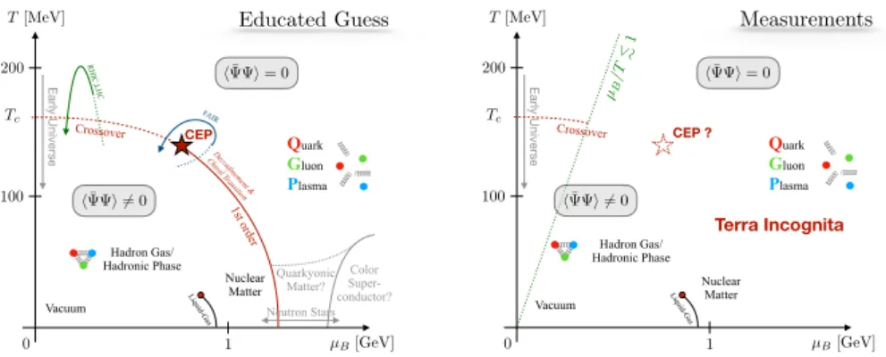
Figure 1.2: Phase diagram of full QCD in terms of temperatureT and baryon chemical potential

µB. Left: It is expected that hadronic phase and the Quark Gluon Plasma are separated by a first

order line at small temperatures and large densities. This line ends in a critical point (CEP) as

a crossover region is connected to it at small densities and temperatures around Tc. The chiral

restoration and deconfinement transition match and the chiral condensate h¯χχican be used as an

order parameter. Right: In fact, only small portions of the phase diagram are settled. While the

nuclear matter transition and a crossover region around Tc are verified, little is known about the

rest of the finite density phase diagram from actual measurements. However, there are many heavy ion colliders probing the essential regions.

accessible by lattice QCD. The order parameter is the chiral condensate [10]

hψψi¯ =h0|ψ(x)ψ(x)|0i¯ =h0|ψ¯R(x)ψ(x)L+ ¯ψL(x)ψ(x)R|0i (1.17)

which is invariant under simultaneous (vector) transformations but not under general chiral rotations. If the chiral symmetry is restored, the chiral condensate vanishes. Otherwise, it has

a non-zero expectation value hψψi 6= 0. Surprisingly, it is observed that the deconfinement¯

phase transition and the chiral transition seem to coincide [21]. This is unexpected as these are related to two distinctly different physical effects. In other words, the chiral transition can indicate at what temperatures quarks and gluons deconfine and transition from the hadronic phase to a Quark-Gluon Plasma. At zero chemical potential the transition temperature is 156.5(1.5) MeV[25]. The main features of the expected phase diagram of full QCD are depicted in Fig. 1.2. In terms of thermodynamic quantities the chiral condensate and the chiral susceptibility are given by

hψψi¯ = T V ∂lnZ ∂mq , χmq = ∂ ∂mqh ¯ ψψi. (1.18)

While the condensate vanishes if the chiral symmetry is restored, the susceptibility forms a peak. Whether the chiral condensate drastically drops to zero when slowly increasing the temperature or if a smooth transition is expected depends on the type of phase transition that takes place. In the same manner the chiral susceptibility can diverge or stay finite depending

(21)

1.3 Lattice Quantum Chromodynamics

on the nature of the phase transition.

There are different schemes that classify the nature of a phase transition. The modern

classificationscheme distinguishes between two broad categories:

1. First-order, discontinuous phase transitions that involve a latent heat due to a fixed amount of energy being absorbed or released. The solid→liquid and liquid→gas transi-tions are of this category.

2. Second-order, continuous phase transitions that have no associated latent heat. These transitions are associated with critical phenomena and characterized by critical exponents. Systems that are filed in the same universality class have matching critical exponents [26].

The QCD phase diagram features a “crossover transition” in Fig. 1.2 which ends in a critical end-point (CEP). The existence as well as the exact location of the CEP is still subject to research. The crossover transition is not a real phase transition since there is no non-analyticity for a definite point with a sensitive order parameter. The phases are continuously connected. In case QCD simulations at vanishing quark masses are considered, denoted as the so-called chiral limit, the crossover becomes a second-order transition which terminates in

a tri-critical point (TCP). The chiral condensatehψψi¯ stays finite along this transition while

the susceptibility is divergent. At large chemical potentials both crossover or second-order transition turn into a first-order transition. In addition to this chiral restoration transition, there is the first-order liquid-gas phase transition of nuclear matter which terminates in a

CEP. Along a first-order transition, bothhψψi¯ and χq are discontinuous.

1.3 Lattice Quantum Chromodynamics

As in all Quantum Field Theories, also QCD has to deal with ultraviolet divergences which spoil calculations, even though the related physical quantities are well-defined and finite. In order to remove these contributions, it is necessary to “regulate” them, i.e. to remove the divergences such that they stay finite. In the low energy regime of QCD the typical perturbative regularization is useless. However, the replacement of continuous space-time by a hypercubic lattice provides the desired ultraviolet (UV) cutoff. This unphysical regulator must be removed in order for calculations to reproduce results in the continuum.

1.3.1 Lattice Regularization

For the regularization of Euclidean space-time, a hyper-cubic lattice Λ is introduced [22]

Λ≡a{n= (n1, n2, n3, n4)|

n = (n1, n2, n3) = 0,1, . . . Nσ−1; n4= 0,1, . . . Nτ−1}

(1.19)

(22)

The four-vectornlabels all of the|Λ|=Q

µNµ=Nσ3×Nτ individual sites which are separated

with respect to their nearest neighbor by the lattice spacinga. Each lattice site location is

therefore addressed as

x∈Λ, xµ=anµ, nµ∈[0, Nµ−1] ∀µ= 1,2,3,4. (1.20)

and consequently, the following replacements have to be taken into account

x→x=na

Z

d4x→a4 X

x∈Λ

. (1.21)

Applied on a function in the momentum this means

f(pµ) = Z dxµe−ipµxµf(xµ)→a X xµ e−ipµxµf(xµ) (1.22)

where the periodicity in the exponential f pµ+ 2π a eν =X xµ e−ipµxµe−2πinνf(xµ) =f(pµ) (1.23)

constraints the momenta to a finite Brillouin Zone as nν ∈Z. The maximum momentum of

p∼1/aacts as the mentioned regulator to render lattice QCD ultraviolet save.

Typically, the spatial volume is considered to be isotropic withN_σ3 =N1·N2·N3. In general

it will deviate from the temporal extent Nσ 6=Nτ.

In the following, lattice sites host quark fields

ψ(x),ψ(x),¯ x∈Λ (1.24)

while the gluon gauge fields will be placed on the links connecting two adjacent sites. They are

represented by the link variablesUµ(x), interconnecting sitex with its neighbor in direction

aeµ=µ.

The main errors in lattice QCD arise from discretization effects and finite volume effects. These can be improved by choosing the spatial extent much larger than the correlation length

aNσ ξ of the particle to be investigated as well as ξ a. As ξ is proportional to the

inverse of the lightest hadron mass, it can be deduced that discretization effects are small if

aM 1, while finite volume effects are small for aM Nσ 1.

Note that due to the lattice discretization, symmetries are violated such as Lorentz symmetry. These are recovered when proceeding towards the continuum limit. This is done by first

extrapolating in the volume V =N_σ3 → ∞denoted as thermodynamic limit and second by

(23)

a → 0 as presented for the discussion of the gauge and fermion part of the discretized

QCD action (see Sections (1.3.2) and (1.3.3)) is not possible, as the only input parameters

are bare parameter, namely the bare coupling g2 = 2Nc/β and the bare quark masses

amu, amd, . . . , amf. Instead of referring to the continuum limit bya→0, the relationβ→ ∞

is used because ofβ∝g−2 and g→0. Discussions on the functional dependence of g(a) via

the Renormalization Group Equation (RGE) (or Callan–Symanzik equation) can be found in [22, 27] and [20].

1.3.2 A Naïve discretization - Gluons

First the Yang-Mills contribution comprising the gluon propagation term of QCD is formulated in terms of lattice degrees of freedom. Such studies where the quarks are considered as infinitely heavy, static objects is referred to as quenched limit with only gluons being the dynamic

variables. Due to the requirement of gauge invariance according to SU(3) transformations, a

gluon field is required to be represented by an appropriate lattice version which is an element of the color gauge group as well. These lattice degrees of freedom are the so-called link

variables Uµ(x). As indicated by their name, the link variables connect two sites which are

required to be nearest neighbors. For the construction of loops it is useful to note that link

variables showing in backward direction U−µ(x) are given as

U−µ(x) =Uµ(x−µ)†. (1.25)

In order to reconstruct the gauge invariant gluonic part of the continuum action S_GCont. =

1 4 R

d4xFµνFµν up to some order in the lattice spacing a, the smallest closed loop build from

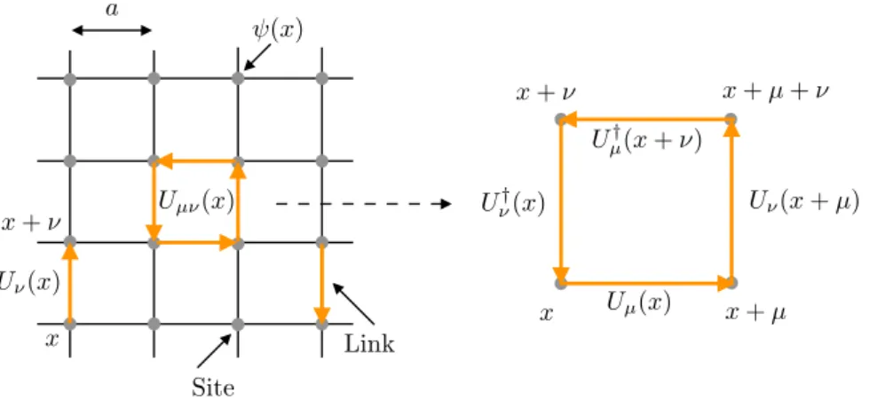
links on the lattice is considered, the so-called plaquette (see Fig. 1.3)

Uµν(x)≡Uµ(x)Uν(x+µ)Uµ†(x+ν)Uν†(x) = _µν(x). (1.26)

Its traced real part is gauge invariant. In fact, the trace of any path ordered product of link variables which forms a closed loop is gauge invariant. Based on the plaquette the Wilson gauge action is formulated [11]

SG(U) =βX x X µ<ν 1− 1 NcRe TrUµν(x) , (1.27)

with the lattice coupling β being related to the bare coupling g via β = 2Nc_g2 . This is the

discrete expression for the continuum gauge action contribution.

In order to ensure that the correct continuum limit can be recovered, the limit a→0 has

to be performed. To do so, the relation of gauge fields Aµ(x) = PN

2 c−1 a=1 Λ a 2 Aaµ(x) and link 9

(24)

Chapter 1 Theoretical Framework x+µ+⌫ x+µ x+⌫ x x Uµ(x) U⌫(x+µ) Uµ†(x+⌫) U⌫†(x) U⌫(x) x+⌫ Link Site a (x) Uµ⌫(x)

Figure 1.3: Left: An isotropic hypercubic lattice. Sitesxdenote where the quark fieldsψ(x)are

placed at. These are connected by linksUµ(x)which have an orientationµand represent the gauge

degrees of freedom. The lattice spacing adenotes the shortest distance between two neighboring

sites. Right: The smallest loop on a lattice, the plaquetteUµν(x)consisting of four links. Its trace

is gauge invariant.

variables in terms of the parallel transporter is recalled

Uµ(x) =Peiag

Rx+µ

x dxµAµ(x)≈eiagAµ(x), (1.28)

withP denoting the path-ordering. The parallel transporter shifts color from a pointxon the

lattice to the adjacent one in direction µ. The plaquette in terms of the gauge field variables

reads

Uµν(x) =eiagAµ(x+µ/2)eiagAν(x+µ+ν/2)e−iagAµ(x+ν+µ/2)e−iagAν(x+ν/2). (1.29)

By utilizing the Baker-Campell Hausdorff formula eAeB =eA+B+12[A,B]+. . . yields

Uµν(x) =eia

2_{g(∂µAν(x)−∂νAµ(x)+ig[Aµ(x),Aν(x)])+O(a}3₎

=eia2gFµν+O(a3), (1.30)

with the field strength tensorFµν(x) =∂µAν(x)−∂νAµ(x)−ig[Aµ(x), Aν(x)] defined just as

the continuum version. Finally, an expansion in the lattice spacinga results in

Uµν(x) = 1 +ia2gFµν−

a4g2

2 FµνF

µν₊_O(a6₎ _(1.31)

which is inserted into the Wilson action Eq. (1.27) with the real part of the trace removing

theO(a2_{)-term of Eq. (1.31). The Wilson action becomes}

SG=a 4 4 X x X µ<ν TrFµνFµν+O(a2). (1.32)

(25)

In the continuum limit the orderO(a2_{) cut-off effects become irrelevant as they vanish for}

a→0. In order to approach the continuum limit faster, there are strategies incorporating

larger gauge invariant loops in the formulation of the gauge action.

1.3.3 A Naïve Discretization - Fermions

This section covers the naïve lattice discretization of the quark fields. For the sake of simplicity, the interacting contribution is disregarded for this discussion such that free fermion fields are described. Therefore, it is the goal to find a formulation for the continuum fermion action

S_Ffree[ψ,ψ] =¯

Z

d4x ψ(x)[γµDµ¯ +m]ψ(x)s (1.33)

in terms of the discretized degrees of freedom, with the covariant derivativeDµ=∂µ+igAµ.

While the prescription from Eq. (1.21) dictates how to convert the space-time integral to a finite sum over lattice sites, the quark fields are placed on the lattice sites according to Eq. (1.24). For the naïve fermion formulation, the derivatives of the quark fields have to be replaced by finite differences. For a symmetric discrete derivative scheme

∂µψ(x)→ 1

2a(ψ(x+µ)−ψ(x−µ)), (1.34)

a lattice version of the free fermion action reads

S_Ffree[ψ,ψ] =¯ a4 X x∈Λ ¯ ψ(x) γµψ(x+µ)−ψ(x−µ) 2a +mψ(x) . (1.35)

This expression is not gauge invariant yet when applying the transformations

ψ(x)→ψ0 = Ω(x)ψ(x), (1.36)

¯

ψ(x)→ψ¯0 = ¯ψ(x)Ω†(x) (1.37)

on the finite difference quark field term, with Ω(x) being an element of SU(3). A gauge

invariant formulation is obtained by introducing the link variablesUµ(x) from Sec. 1.3.2 which

transform according to

Uµ(x)→U_µ0(x) = Ω(x)Uµ(x)Ω†(x+µ). (1.38)

Thus, the naïve action for fermions in an external gauge fieldU reads

SF[ψ,ψ, U] =¯ a4 X x∈Λ ¯ ψ(x) γµ Uµ(x)ψ(x+µ)−U−µ(x)ψ(x−µ) 2a +mψ(x) (1.39) =a4 X x,y∈Λ ¯ ψ(x)M(x, y)ψ(y). (1.40) 11

(26)

In the last line the bilinear structure was identified, with the naïve lattice Dirac operator (or fermion matrix) given as

M(x, y) = 1

2a X

µ

γµ[Uµ(x)δ(x+µ, y)−U_µ†(x−µ)δ(x−µ, y)] +mδ(x, y). (1.41)

For a→0, the link variables from Eq. (1.28) are Taylor expanded

Uµ(x)≈1 +iagAµ(x) +O(a2)

U−µ(x)≈1−iagAµ(x−µ) +O(a2)

(1.42)

and inserted in the action Eq. (1.39)

SF[ψ,ψ, U] =a¯ 4X x∈Λ ¯ ψ(x)   4 X µ=1 γµ _ψ(x₊_µ)₋_ψ(x₋_µ) 2a + iagAµ(x)ψ(x+µ) +iagAµ(x−µ)ψ(x−µ) 2a +mψ(x) +O(a) =a4X x∈Λ ¯ ψ(x) [γµ(∂µ+igAµ(x))ψ(x) +mψ(x)] +O(a). (1.43)

In the last line it is used that ψ(x±µ) = ψ(x) +O(a) and Aµ(x−µ) = Aµ(x) +O(a).

Additionally, the continuum derivative is already reintroduced to highlight the similar structure to Eq. (1.33).

In comparison, the fermionic part of the action provides an error in the lattice spacing of

order O(a) while for the gauge part it is O(a2_{). Note that the naïve discretization scheme is}

only one choice to reproduce the continuum action.

The final partition sum, taking into account the gauge-invariant measure on the lattice reads

Z = Z Y x∈Λ dψ(x)dψ(x)¯ Z Y x∈Λ 3 Y µ=0 dUµ(x)e−SF[U, ¯ ψ,ψ]_e−SG[U] _(1.44)

The naïve lattice discretization introduces a major drawback in the form of the doubler problem which is explored hereafter.

1.3.4 Doubling Problem

In the following, the doubling problem is explored that hinders the use of the naïve fermion

discretization. For the free fermion action, i.e. Uµ(x) =1, the Dirac operator Eq. (1.41) in

momentum space reads

˜ M(p) =m·1+ i a 4 X µ=1 γµsin(pµa) (1.45)

(27)

1.3 Lattice Quantum Chromodynamics 1 a ⇡ 2a ⇡ 2a ⇡ a ⇡ a 1 a f(pµ) _pµ ˜ pµ=sin(pµa) a pµ

Figure 1.4:The naïve lattice discretization gives rise to the momentum pµ˜ = sin(pµa)/a which

becomes zero at additional locations±π/2within the Brillouin Zone. In comparison, the continuum

momentumpµ has a simple zero at0. In four dimensions this gives rise to16poles or so-to-say

15unwanted doublers. (Figure inspired by [20])

which has to be inverted in order to give rise to the fermion propagator [20] ˜ M(p)−1=m−i P µγµpµ˜ m2₊P µp˜2µ , (1.46)

where ˜pµ is given by ˜pµ= sin(pµa)/a(see Fig. 1.4). For ˜pµ→pµ the continuum propagator

is obtained m=0 ⇒ a→0 −iP µγµpµ p2 . (1.47)

This propagator has a single particle pole atpPhys= (0,0,0,0) for massless fermions. However,

the discrete lattice version does not just have a single pole at zero momentum but it is spoiled by the Sine-function which introduces additional contributions. Within the Brillouin Zone

there are 15 additional locations where the Sine-function becomes zero forpµ=π/2. These

correspond to the edges of the Brillouin Zone

pEdge={(π/2,0,0,0),(0, π/2,0,0), . . . ,(π/2, π/2, π/2, π/2)} (1.48)

with a doubling in the number of particles with each dimension. In four dimension there are

2d= 15 + 1 = 16 poles, 15 unphysical and a single physical relevant one.

Thus, the naïve discretization produces Nf·2d particles which do not vanish in the limit

a→0. This is the motivation for the use of different fermion actions, such as the staggered

formulation, which try to cancel out the doublers with additional contributions. These

(28)

contributions are required to vanish in the continuum limit as well. A limitation concerning the construction of lattice fermion formulations is given by the Nielsen–Ninomiya theorem. This theorem states that there is no fermion action without doublers that has all the following properties [28]:

• Continuum chiral symmetry ({D, γ5}= 0) in massless case

• Locality of the fermion operator

• Correct continuum limit

Hence, there are various approaches to discretize fermions in order to tackle the doubling problem. For Wilson fermions all doublers are removed, however, chiral symmetry is explicitly broken. In contrast, the idea of staggered fermions is to reduce the number of doublers by a factor of four, such that doublers will remain in the continuum, however, also chiral symmetry is partly kept restored.

The fermion doubling phenomenon is strongly related to the existence of the chiral anomaly. While in the continuum the anomaly arises from the chiral non-invariance of the path integral measure [23], for the lattice version it is the non-invariance of the Lagrangian.

1.3.5 Staggered Fermions

In order to work towards the staggered formulation, a symmetry of the naïve action is utilized which reduces the number of doublers by a factor four. This four-fold degeneracy is obtained by a local transformation of the fermion fields (spin-diagonalization)

ψ(x)→Ω(x)ψ0(x), ψ(x)¯ →ψ¯0(x)Ω†(x), (1.49)

with a total of sixteen different transformation matrices Ω defined as [29]

Ω(x) =γ₀x0γ₁x1γ₂x2γ₃x3 andxµ∈(0,1). (1.50)

This transformation is used to remove theγµ dependence from the naïve fermion description

by applying

ηµ(x)≡Ω†(x)γµΩ(x) =(−1)x0+x1+x2+x3

Ω†(x)Ω(x) =1.

(1.51)

The newly introduced staggered phasesηµ(x) take over the role of the γµ matrices such that

the whole action S will be diagonal in Dirac space. The phases are constraint by

ηµ(x)ην(x+µ)η_µ†(x+ν)η_ν†(x) =−1 ⇒ηµ(x) =(−1) P ν<µ xν . (1.52)

(29)

Finally, the fermion action acquires the form

S =X x∈Λ 3 X α=0  ψ¯_α(x) 3 X µ=0 ηµ(x) Uµ(x)ψα(x+µ)−ψα(x−µ)Uµ†(x−µ) 2a ! +mψ¯α(x)ψα(x)   (1.53)

Each component of the Dirac spinor labeled by α yields the same term. Because of being

diagonal, three of the four components can be discarded and the one-component fieldχ is

introduced. This reduces the number of Dirac particles in the continuum from 16 to four. In

order to distinguish these four continuum quark flavors, the termtaste is introduced. With

the newly defined one-component fieldsχ the gauge invariant staggered action reads

Sstagg(µ) =X

x∈Λ 1 2a

"

η0(x)γχ(x)¯ eaτµqU0(x)χ(x+ 0)−χ(x−0)e−aτµqU₀†(x−0)

+ d X i=1 ηi(x) ¯χ(x)Ui(x+ 0)χ(x+i)−χ(x−i)U_i†(x−0)+mχ(x)χ(x)¯ # (1.54)

where it is incorporated that general lattice simulations with staggered fields are performed

on anisotropic lattices aσ 6= aτ, thus, accounting for the bare anisotropy parameter γ.

Furthermore, a quark chemical potential contribution is incorporated.

There are a total of 16 one component fields, each with a different phase factor, corresponding

to the sites of a 24 _{hypercube. Each such staggered fermion with its 16 components can be}

seen as four tastes of continuum fermions each with four Dirac components. Note that the taste-symmetry of rotations is broken by a discrete lattice leading to a mass splitting of the taste multiplets [30].

In contrast to Wilson fermions, the staggered formulation keeps a remnant chiral symmetry.

This is stressed by considering the transformation of γ5. According to Eq. (1.49) this is given

by [22]

¯

ψ(x)γ5ψ(x) =η5(x) ¯ψ(x)0ψ(x)0. (1.55)

Thus, the site-dependent staggered phase (x)≡η5 = (−1)x0+x1+x2+x3 substitutes γ5. In the

chiral limit the staggered action is then invariant under continuous transformations

χ(x)→eiα(x)χ(x), χ(x)¯ →χe¯ iα(x). (1.56)

This is the global chiral symmetry for the staggered quark degrees of freedom that are distributed over the hypercube.

A further reduction of the number of doublers can be achieved by applying the rooting procedure where the quartic (square) root is taken from the four-flavor staggered determinant

(30)

det[M] yielding one (two) flavors.

Within this dissertation, staggered fermions based on the action Eq. (1.54) are used.

1.3.6 Finite Temperature and Density

Lattice studies at finite temperature and density are of interest in order to investigate QCD matter in the early stages of the universe and the condensation of hadrons during the cooling process [22].

Finite Temperature The infinite space-time volume limit corresponds to QCD at zero

tem-perature. However, as implied by the continuum discussion of Equations (1.3) and (1.4) a

non-zero temperature is achieved by restricting the physical extent of time to β while the

spatial volume is still be considered in the infinite volume limit. The corresponding fields are periodic (bosons) or anti-periodic (fermions) in time. While the spatial contribution is still considered in the infinite volume limit, the Euclidean lattice time extent is associated with

β =aNτ = 1

T. (1.57)

The limitβ → ∞ corresponds toT →0. At finite spatial volume and finite temperature the

continuum limit is achieved bya→0 while aNσ andaNτ are kept fixed.

Finite Density For QCD matter the net quark number density is non-vanishing. This is

accounted for by considering a non-zero quark chemical potential which yields the grand canonical ensemble

Z(T, µ) = Trhe−β(H−µqNq)i, (1.58)

with the quark numberNq. Alternatively, the baryon number NB=Nq/3 and the baryon

chemical potential µB = 3µq can be used. Since Nq and NB are integer valued, the grand

canonical partition function can be expanded in a power series

Z(T, µ) =X

n

eµq/TnZ(T). (1.59)

This expansion is referred to as fugacity expansion with the fugacity variableeµq/T and the

quark numbern∈Z[22].

The finite density sign problem arises when integrating out the fermionic contribution to the partition function which results in the fermion determinant Eq.(1.5) which depends on the

chemical potential. For µ= 0 the fermion matrix exhibits γ5 hermicity which leads to