longitudinal data - heroin users
receiving methadone
CHIEN-JU LIN
STATISTICAL SCIENCE University College London
A thesis for the degree of Doctor of Philosophy October 2014
I confirm that the work presented in this thesis is my own. Where infor-mation has been derived from other sources, I confirm that this has been indicated in the thesis.
Name: CHIEN-JU LIN
Signature:
I would like to express my sincere gratitude to everyone who supported me throughout my PhD study.
I would like to express the deepest appreciation to my PhD supervisor Dr. Christian Hennig for the continuous support of my research, for his patience, enthusiasm, and vast knowledge.
I would also like to thank my second supervisor, Dr. Ioannis Kosmidis, and thesis committee, Prof. Tom Fearn and Prof. Sabine Landau, for their encouragement and insightful comments.
I thank my fellows at the Department of Statistical Science. In particular, I am grateful to Oya Kalaycioglu and Khadijeh Taiyari for the stimulating discussions and for all the fun we had. Special thanks to Tsu-Jui Cheng, Saul Holding, Maurice Lyver, Yu-Chia Shih, and Ying-Li Wu for their en-couragement and support.
Last but not the least, I owe my deepest gratitude to my family: my par-ents, my lovely sister and brother, my adorable nephews for supporting me spiritually throughout my life.
Methadone is used as a substitute of heroin and there may be certain groups of users according to methadone dosage. In this work we analyze data for 314 participants of a methadone study over 180 days. The data, which is called category-ordered data throughout this study, consists of seven cate-gories in which six catecate-gories have an ordinal scale for representing dosages and one category for missing dosages. We develop a clustering method involving the so-called p-dissimilarity, modification of Prediction Strength (PS), a null model test, and two ordering algorithms. (1) The p-dissimilarity is used to measure dissimilarity between the 180-day time series of the par-ticipants. It accommodates categorical and ordinal scales by using a param-eter p as a switch between data being treated as categorical and ordinal. It measures dissimilarity between observed dosages and missing dosages by using a parameter β. Also, it could be applied in a wider field of applica-tions, such as survey studies in which questions use choices on the Likert scales and a don0tknow-category. (2) The PS determines the number of clusters by measuring the stability of clusters, and the Average Silhouette Width (ASW) measures coherence. We propose rules to modify PS so that it can be fully applied to hierarchal clustering methods. Next, instead of preselecting a clustering method, we let the data to decide which clustering method to use based on cluster stability and cluster coherence. The parti-tion around medoids (PAM) method is then selected. (3) We propose the null model test to determine the number of clusters (k). Many methods for the determination of number of clusters give values for k ≥ 2 based on cluster compactness and separation, and suggest to use the k with the highest value. Viewing this question from a different perspective, for a fixed k and a selected clustering method, the null model test uses a null model and parametric bootstrap to explore the distribution of a statistic under the
in which the distributions of the categories are the same as those of the real data. We apply the null model test to investigate whether the clusters found according to PAM and ASW/PS can be explained by random varia-tion. (4) We use heatplots to evaluate the quality of clustering. A heatplot is a graph that represents data by colour. It consists of horizontal lines representing the data for objects. However, the interpretability of a heat-plot strongly depends on the location of the objects along the vertical-axis. We propose two algorithms to locate objects on a heatplot. The first algo-rithm using multidimensional scaling (MDS) is for general use. The second algorithm using projection vector is for the PAM method. Each of them locates objects in a heatplot. The heatplot can then be used for informa-tion visualisainforma-tion. It displays clustering structures, relainforma-tionships between objects and clusters in terms of their dissimilarities, locations of medoids, and the density of clusters. Despite the fact that no significant clustering structure is observed, the sequences of categories for clusters are clinically useful. The sequences of categories indicate detoxification. Our data shows participants with low heroin addictions attempted to reduce/quit the use of methadone at the third month. As for participants with high addictions, few attempted to reduce the use of methadone at the fifth month and most required more time to finish the detoxification process. Also, we find the heroin onset age might have an influence on the patterns of detoxification.
The following notations, abbreviations and defined terms are used throughout this the-sis. They are also introduced in their first occurrence in each chapter.
Symbol Definition and Explanation k denotes the number of clusters
xit denotes data for the tth variable for objecti.
xi represents data for objecti.
d(., .) denotes dissimilarity between variables
D(., .) denotes dissimilarity between objects\ clusters Ci denotes a category i, representing a set of dosages
δii0(t) is equal to 1 when both objects iandi0 for theirtth values are non-missing,
and equal to 0 otherwise.
p is a tuning constant, 0< p <1, for measuring dissimilarities between objects. αii0(t) refers to dissimilarity between thetth values for objects iand i0.
It is set to the absolute value of the difference between thetth values
β(t) refers to dissimilarity between thetth values in which one or both of them are missing values.
Symbol Explanation
MMT Methadone Maintenance Therapy
ASW(k) Average Silhouette Width index forkclusters PS Prediction Srengh
MDS Multidimensional scaling
Dosage314 dosage data for the 314 participants for 180 days CO314 category-ordered data for the 314 participants
Term Definition
stable methadone dosage means that categorized dosage for a participant consists of long sequences of categories.
initial date means the first date on which a participant joined the MMT. category-ordered data means the data that consists of categories, referring to
List of Figures x
List of Tables xiii
1 Introduction 1
1.1 Background . . . 1
1.2 Motivation . . . 3
1.3 Outline . . . 9
2 Methadone Maintenance Therapy (MMT) 12 2.1 Literature review of methadone . . . 12
2.2 MMT database . . . 14
2.2.1 Data for prescription and dosage taken . . . 15
2.3 Number of participants . . . 18
2.3.1 Records of prescription and dosage taken for the initial sample . 19 2.3.2 Selection of the meaningful sample . . . 21
2.4 A new data format : category-ordered data . . . 24
2.4.1 Category-ordered data: CO314 . . . 25
2.4.2 Imputation of the category-ordered data . . . 29
3 Dissimilarity functions and clustering methods 35 3.1 Dissimilarity functions . . . 35
3.2 Hierarchical clustering and partitioning methods . . . 42
3.2.1 Linkage methods . . . 43
3.2.2 Partition clustering methods . . . 45
4 New dissimilarity function : the p-dissimilarity 50
4.1 Motivation of dissimilarity design . . . 50
4.2 Dissimilarity between categories . . . 52
4.3 Design of the p-dissimilarity . . . 55
4.3.1 The p-dissimilarity without missing values . . . 55
4.3.2 The p-dissimilarity with missing values . . . 58
4.4 Advantages and disadvantages of the p-dissimilarity . . . 60
5 Determination of the number of clusters 63 5.1 Indexes for finding of number of clusters . . . 63
5.2 Average Silhouette Width . . . 65
5.3 Prediction Strength . . . 66
5.3.1 New rules for modifying the Prediction Strength . . . 69
6 The clustering method and number of clusters for CO314 77 6.1 Determination of β,p, and clustering method . . . 77
6.1.1 Determination of β . . . 77
6.1.2 Determination of the clustering methods . . . 80
6.1.3 Determination of p . . . 80
6.2 Null model test . . . 81
6.2.1 Motivation . . . 81
6.2.2 Proposed null model test . . . 85
6.3 Application of the null model test to CO314 . . . 88
6.3.1 Exploration of movements of categories in CO314 . . . 90
6.3.2 The null model for CO314 . . . 98
6.3.3 Determination of the number of clusters . . . 100
7 Visualisation of the PAM results 105 7.1 Motivation . . . 105
7.2 Multidimensional scaling . . . 110
7.3 Order of clusters . . . 111
7.4 Order of objects within clusters . . . 112
7.4.1 Ordering by multidimensional scaling . . . 112
7.5 Comparison of CO314 and the reference datasets . . . 119
8 Sensitivity analysis, stability analysis and features of the final five clusters 126 8.1 Sensitivity analysis . . . 126
8.2 Comparison between CO314 and the imputed datasets . . . 129
8.3 Result of dosage patterns . . . 130
8.4 Demographical information relating to the five clusters . . . 134
9 Conclusion and discussion 139
1.1 Schematic representation of the organization of the contents of the thesis 11
2.1 The number of participants over 732 days. . . 19
2.2 Records of dosage taken for the 1257 participants for 732 days. . . 22
2.3 The dosage taken records for 314 participants over 180 days. . . 24
2.4 Number of prescriptions for the 313 participants over 180 days. . . 25
2.5 Records of prescriptions and dosage taken for two selected participants from day 1 to day 180. . . 26
2.6 Heatplot of Dosage314 and that of CO314 . . . 32
2.7 Illustration of imputation: original data. . . 32
2.8 Illustration of imputation: imputed data in which among the records of category 7, some of them are imputed. . . 33
2.9 Heatplot of ImpCO314 and heatplot of ImpCO7314 . . . 33
2.10 Illustration of imputation for missing records . . . 34
2.11 Heatplot of ImpDosage314 . . . 34
3.1 Illustration the Euclidean distance and the DTW . . . 40
3.2 An illustration of a dendrogram . . . 44
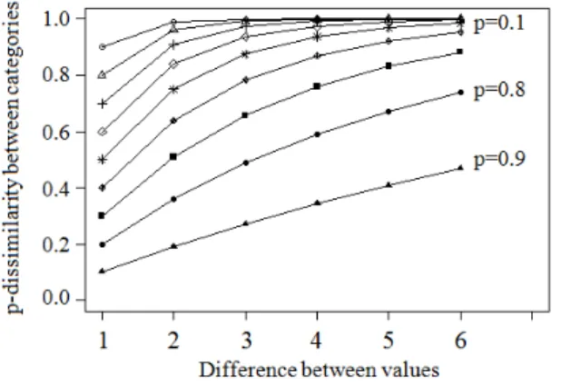
4.1 An illustration of p-dissimilarities . . . 56
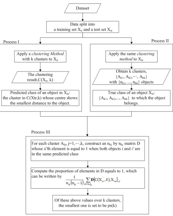
5.1 Flowchart of the Prediction Strength. . . 67
5.2 Application of the new rules onC(Xtr,2) . . . 71
5.3 Simulated datasets . . . 73
6.2 The average Prediction Strength for the four clustering methods for 2 to 20 clusters . . . 82 6.3 The Average Silhouette Width for the four clustering methods for 2 to
20 clusters. . . 83 6.4 Distributions of the number of participants in the seven categories. . . . 89 6.5 The average relative frequencies ofψ1 . . . 96 6.6 The relative frequency of ψ2. . . 97 6.7 Relative frequencies from category 7 to categories 1 to 7. . . 100 6.8 Test of each number of clusters for CO314 for the PAM method with the
average Prediction Strength. . . 101 6.9 The null model test with average Prediction Strength. . . 102 6.10 Test of the homogeneity between the null model and CO314 for the ASW. 103 6.11 Test of the homogeneity between the null model and CO314 with ASW . 104 6.12 The null model test with ASW. . . 104
7.1 The hierarchical tree of the Average Linkage and the heatplot of the p-dissimilarity matrix of CO314 . . . 107 7.2 Heatplot of p-dissimilarity matrix of CO314 with random orders within
clusters. . . 108 7.3 Heatplot of p-dissimilarity matrix of CO314 by seriation. . . 109 7.4 Heatplot of Dosage314and heatplot of the p-dissimilarity matrix of CO314
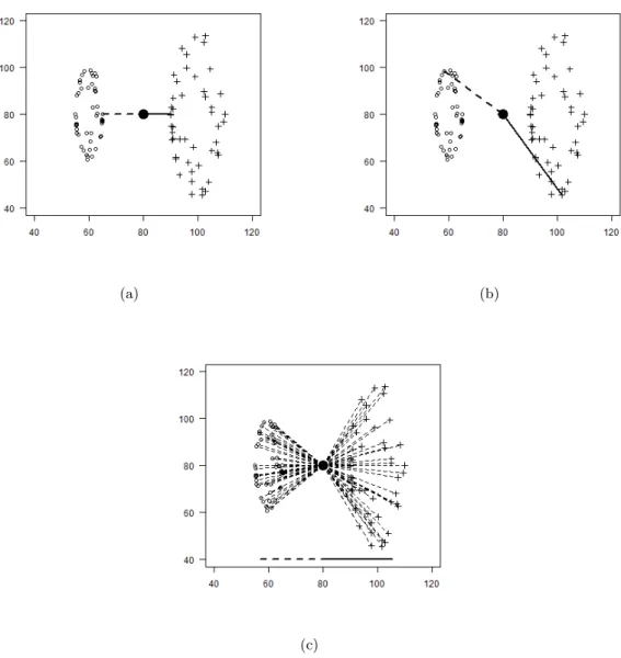
with the order of participants generated from MDS on all participants belonging to the same and the neighbouring clusters. . . 114 7.5 Illustration of the planes . . . 115 7.6 Illustration of representing the dissimilaty between x(j) and x(j−1) by a
vector . . . 116 7.7 Illustration of standardized projection of an object . . . 117 7.8 Heatplot of Dosage314 and heatplot of the p-dissimilarity matrix with
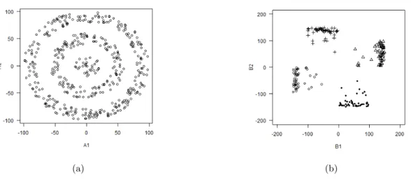
the order of the participants obtained by using projection vectors. . . . 119 7.9 The heatplots of simulated CO314. . . 123 7.10 The heatplots of the p-dissimilarity matrix of simulated CO314. . . 124
8.1 Heatplot of Dosage314 and of the p-dissimilarity matrix of ImpCO314 with the order obtained by the algorithm of the projections. . . 131
8.2 Frequency of the categories from day 1 to day 30 for the five clusters. . 135 8.3 Frequency of the categories from day 31 to day 180 for the five clusters. 136 8.4 The movement of clusters over time . . . 137
2.1 Illustration of the data recording process. . . 16
2.2 Frequency of prescription dosage of the 1252 participants. . . 20
2.3 Number of participants of various attendance rates. . . 21
4.1 The p-dissimilarity matrix of the seven categories with β= 2. . . 60
5.1 The average Prediction Strength of dataset A . . . 75
5.2 The average Prediction Strength of dataset B . . . 76
6.1 The frequency ofα . . . 79
6.2 Relative frequencies from category 1 to categories 1 to 6 over 22 days. . 94
6.3 Relative frequencies from category 2 to categories 1 to 6 over 22 days. . 95
6.4 The estimated transition probabilities matrix forψ1 . . . 99
7.1 The frequencies of answers to each question in the survey. . . 125
8.1 The contingency table of the two clustering results. . . 128
8.2 Stability of the p-dissimilarity ofp= 0.6 to the found clusters. . . 129
8.3 The crosstable of the clustering result of CO314 and that of ImpCO314. 131 8.4 The mean and standard deviation of dosage of the five clusters. . . 132
Introduction
1.1
Background
Drug abuse creates problems in society and the economy. The statistical news released by the Ministry of Justice of Taiwan in 2010 showed that among all arrests for drug abuse violations, 74.2% of them were arrested on charges of Schedule I drugs, defined as drugs with a high potential for abuse and highly addictive. Schedule I drugs include heroin, opium, morphine, etc. Moreover, there was an increasing trend in the number of arrests for abusing Schedule I drugs over the years. Winick [1962] found addicts mature out of addiction as a reflection of their life cycle or they mature out of addic-tion as a funcaddic-tion of the length of their addicaddic-tion. Termorshuizen et al. [2005] showed that the concept of “maturing out” to a drug-free state did not apply to the majority of drug users. Also, Termorshuizen et al. [2005] examined harmfulness to drug users by the mortality rates and reported at least 27% of drug users died within 20 years of starting regular drug use.
Among the abuse Schedule I drugs, heroin is the most expensive and highly addic-tive. Heroin-dependent individuals who aim at overcoming their addiction are offered a methadone maintenance therapy (MMT) for many years. The main purpose of the MMT is not to help them to achieve abstinence but to minimize the harm associated with the use of heroin (Ball and Ross [1991]; Ward et al. [1999]). Research showed that MMT had a positive effect on drug users and on society (Gossop et al. [2000]; Marsch [1998]; Masson et al. [2004]; McLellan et al. [1985]; Powers and Anglin [1993]; Strain
et al. [1993a,b]). The effect of methadone lasts 24 hours and consequently it has to be taken on a daily basis. To date there is no clear principle for the determination of the methadone dosage. Physicians prescribe dosages based on their own intuition.
Some researchers studied methadone dosages. Maxwell and Shinderman [2002] re-ported that higher methadone dosages (above 100 mg/day) were more effective in treat-ing heroin addicts, while Maremmani et al. [2003] observed that many heroin addicts had positive outcomes with lower dosages. Both high and low dosages are consid-ered as good prescriptions. There is no principle for determining proper methadone dosages. Some researchers studied the association between methadone dosages and groups. Langendam et al. [1998] observed that the mean methadone dosage was higher for ethnic west Europeans, older drug users, HIV-positive drug users, longer duration of methadone use and so on. Murray et al. [2008] surveyed 54 participants from a methadone maintenance clinic and found that methadone dosage might be uniquely re-lated to the personality disorders. On the other hand, Gossop et al. [2000] performed a one year follow-up study on 478 participants. The Euclidean distance K-Means cluster-ing method was used to group their study participants by the frequency of their illicit drug use over time. Four groups were identified and two groups showed substantial reductions in their illicit drug use and criminality. They concluded that the methadone dosage might be related to a certain group in which MMT was appropriate. Their works were limited in using self-reported data that was not reliable but their finding might be clinically useful. It was possible that high/low dosage was better in treating some groups of people. However, due to the unreliable data, they failed to address how to find the certain group.
Ideally, drug users are expected to reduce the use of heroin by addicting to methadone and then to quit use of methadone. The dosages should consequently have a pattern in which they go up at the beginning of the treatment and later go down. This would indicate detoxification. Physicians think participants with such a dosage pattern and a high attendance rate, most will have a positive outcome. Therefore, we are interested in the participants’ behaviour, that is, patterns of daily methadone dosage.
An MMT project was launched by a hospital in Taiwan. The project provided an opportunity to acquire more information about this therapy and offered an opportu-nity to obtain more insight into MMT by assessing patterns of daily methadone dosage administered to participants. Two types of methadone dosage were recorded by an MMT database system, one being the dosage of their weekly prescriptions prescribed by physicians and the other the daily dosage they had taken recorded by pharma-cists. Participants would occasionally have multiple prescriptions but only one record of dosage taken in a single day. Besides, there were occasions on which participants abused drugs and took methadone at the same time, so participants were allowed to take dosage that was lower than the prescribed dosage to avoid overdosing. Of those who continued to abuse heroin while receiving the MMT, there were some fluctuations in their dosage taken records as a result of their demand for daily methadone differ-ing. By and large, following a weekly prescription, a participant took methadone daily for a period of seven days. The prescription records were constant over every 7-day period, whereas the dosage taken records varied over time. Moreover, many partici-pants dropped-off from MMT and returned days later, which resulted in lots of missing data in their dosage taken records. These missing records were not missing at random. Although the numerical daily methadone dosage contains variation and non-random missing values, these records were considered to be a more reliable data. More details of the MMT data can be found in Chapter 2.
The aim of our work is to develop a method to divide participants into groups and then find the differences between the groups. Unfortunately, without the data of whether participants achieve abstinence or not, we do not understand the relationship between treatments and final outcomes. However, by clustering, we can study about the association between dosage patterns and demographic factors, the degrees of addictions, retention of MMT. Also, the dosage patterns provides the possibility of developing a guideline for prescribing a proper methadone dosage.
1.2
Motivation
The initial prescription dosage for the participants who had no experience of methadone was 20 mg. The physicians adjusted the dosage of methadone every seven days after
dis-cussing with participants their preferred prescription dosage settings. 10 mg was often used as a unit of adjustment of prescription dosage. While receiving MMT, partici-pants reported the frequency of their drugs use, from which physicians could measure the effectiveness of the MMT. However, this kind of self-reported data was not reliable and not validated. The physicians of the MMT project observed that abused drugs would reduce the demand of daily methadone. As a result, there were fluctuations or missing values in the dosage taken records. These fluctuations reflected the patterns of drug abuse. There were reasons for which participants abused drugs. One of which was they did not believe in the treatment. Ball and Ross [1991] said participants who remained for more than six months had a marked drop in their drug abuse. However, they found, on average, 11 % (200/1800) of people who commenced MMT after inquiry. Besides, only 38 % of them stayed in the therapy after a year. The physicians of the MMT project in Taiwan suspected that early drop out might be caused by participants having no confidence in methadone.
As aforementioned, drug users are expected to have a dosage pattern which goes up at the beginning of the treatment, followed by a period of stable dosage, and then goes down. The physicians believe that of those with such an up-stable-down pattern and a high attendance rate during the treatment period, most will have a positive outcome. On the other hand, those whose daily methadone dosage fluctuates can be interpreted as lacking motivation.
Our idea starts from identifying patterns. We define a methadone curve by joining all daily dosages with a line. Methadone curves are a remarkable tool to show detoxi-cation. By identifying the patterns of methadone curves, we can correct participants’ behaviours of taking dosage to the right track. We mean to convince participants that the dosage is right for them and lead them to have an up-stable-down curve. Since how long participants have been abusing heroin, the degrees of their addictions, the drug abuse history and some unknown factors might all have an influence on the pat-terns of detoxication. There might be more than one concave curve. Therefore, we attempt to develop a clustering technique that is capable of dividing the MMT partic-ipants into subgroups for finding dosage patterns of clusters. These patterns can then
be used as a guideline for determining proper methadone dosages to increase partic-ipants’ trust in MMT and to reduce the rate of quitting the treatment at an early stage.
The central problems of clustering the participants in our study are the fluctua-tions of dosages and missing dosages. First of all, some participants who abused heroin while receiving the MMT did not need the full dosages indicated on their prescrip-tions to accommodate their addicprescrip-tions. In fact, they took a combination of drug and methadone in order for their addictions to be satisfied, so it was not guaranteed that the methadone dosages they took indeed represented detoxication. Secondly, missing dosages were not missing at random. They were recorded as zeroes but the addic-tions should not be zeros. These zeros appeared as sequences. In some cases, a long sequence of zeros point to more severe problems of the participant, or a tendency to leave the study, or illicit drug use. We take account of these issues and propose to categorize dosages for alleviating the fluctuations of observed dosages and for keeping the sequences of missing dosages. The ranges of observed dosages for categories are based on the recommendations of physicians. Participants whose actual dosage is in the range of 20 mg, that is, dosage between 1 and 20 mg, between 21 and 40 mg, between 41 and 60 mg, between 61 and 80 mg, between 81 and 100 mg, can be considered as the same. We define a new data format. The new data consist of seven categories in which six categories have an ordinal scale for representing dosages and one category for missing dosages. Throughout the study we use the term “category-ordered data” to refer to this new data. The methadone curves will then be represented by sequences of categories. The aim of this study is thus to find clusters in which participants have similar long sequences of categories.
Two issues arising in applied cluster analysis are the selection of the clustering method and the determination of the number of clusters. Among clustering methods, we focus on dissimilarity-based clustering methods because the features of our data make the model based clustering methods hard to applied straightforward (see Section 3.3 for details). We review the Single Linkage, the Complete Linkage, the Average Linkage, the K-Means and the partitioning around medoids (PAM) (Gordon [1999]; Hartigan and Wong [1979]; Kaufman and Rousseeuw [1990]). The Single Linkage de-fines the dissimilarity of two clusters as the shortest distance between two objects,
while the Complete Linkage defines the dissimilarity as the furthest distance between two objects. The Average Linkage, instead, utilizes the average of all distances of ob-jects of two clusters. As for the K-Means and the PAM clustering method, the former partitions objects into k clusters in which each object is assigned to the cluster with the nearest mean vector, while the latter partitions objects into k clusters in which each object is assigned to the cluster with the closest medoid. Note thatkis a positive integer and has to be decided first. The clustering methods group together objects that are considered as similar. The criterion of considering two objects or sets as similar is defined by dissimilarity functions. The dissimilarity functions play the role of con-necting the researcher’s goals, features of the data and scientific knowledge (Gordon [1990]; Hennig and Hausdorf [2006]). There is a considerable amount of literature on dissimilarity functions. Many attempts are made with respect to study purposes. For example, in the gene research of Luca and Zuccolotto [2011] and the financial research of Douzal-Chouakria et al. [2009], they proposed new dissimilarity functions which adapt the features of their data. To the best of our knowledge, a dissimilarity function for data in which variables have both categorical and ordinal characters has not yet been established. Therefore, we propose a so-called p-dissimilarity. The p-dissimilarity is used to measure dissimilarity between the 180-day time series of the participants. It accommodates categorical and ordinal scales by using a parameter p as a switch be-tween data being treated as categorical and ordinal. It uses a parameterβ to tune the dissimilarity involving missing values compared to the distances between non-missing values. Also, it could be applied in wider fields of application, such as survey studies in which questions use choices on the Likert scales and adon0tknow-category.
As for the determination of the number of clusters, it is impossible to prove which index is the best mathematically. Researchers try to use simulation studies to under-stand the performance of index. Milligan and Cooper [1985] examined 30 indexes and showed that the Calinski and Harabasz index (Calinski and Harabasz [1974]) had the best performance. Arbelaitz et al. [2013] carried out a similar study, which included many indexes that did not exist in 1985. They found that six indexes had better perfor-mance. Our cluster analysis is performed based on the p-dissimilarity, so indexes that can cooperate with it will be considered. The Average Silhouette Width (ASW) (Kauf-man and Rousseeuw [1990]; Rousseeuw [1987]), which is one of the six indexes, is thus
used in our study. This index measures coherence of clusters. Besides, a more recent index called Prediction Strength (PS) (Tibshirani et al. [2001]) is also used. This index measures stability of each cluster in terms of similarity between clustering results. We focus on these two index, one measuring coherence and the other measuring stability. The PS index can cooperate with the p-dissimilarity, albeit with a modification. The concept of the PS was to view an analysis of clustering as an analysis of classification. At the beginning of the algorithm, a dataset is partitioned into a training set and a test set. Then, for objects in the test set, the algorithm compares their “predicted class” and their “true class”. If a hierarchical clustering method is used, the true class is built based on the hierarchical clustering method. However, the predicted class is built on the basis of the K-Means method. This brings an issue of measuring stability of clustering results obtained by hierarchical clustering methods. Therefore, we propose new rules for modifying the PS when the hierarchical clustering methods and the PAM method are used. Also, the ASW and modified PS are used for selecting clustering methods. We let the data to select the clustering method based on cluster stability and coherence.
Moreover, the information of k is rarely previously known, so indexes for determi-nation of the number of clusters produce values for every k >1 on the basis of cluster compactness and separation, and yet only onek will be used. For some indexes, thek which scores the highest value is used, while for other indexes, the firstk with a value above a threshold is used and, for other indexes, thekfor which there is a gap between its value and that of (k+ 1) is used. An area of rationale behind decisions of whichkto use is not widely understood. We attempt to view the question of determining the num-ber of clusters from a different position. Instead of comparing values fork= 2, . . . , K, for a fixedk, we compare its value to the distribution of the test statistic under the null assumption. The null assumption is that there is no cluster. We propose a null model test to test if the dataset is homogeneous. The null model test involves a null model and parametric bootstrap. The null model fits all non-clustering aspects of the real dataset, such as relationships between variables, time dependency, marginal distributions and etc. The parametric bootstrap is used to draw reference datasets from the null model. These reference datasets are used to construct the distribution of the test statistic. The distribution of the test statistic is used to explore whether the found number of clusters can be explained by random variation. Also, we define a single test of the homogeneity
hypothesis against a clustering alternative by aggregating the test results for differentk.
In addition, assessing the quality of clustering results is also of interest. Some research has been conducted on information visualisation via heatplots of row data matrices and of proximity matrices (Chen [2002]; Hahsler and Hornik [2011]; Hahsler, Hornik, and Buchta [2008]; Wu, Tien, and Chen [2010]). A heatplot is a graph that represents data by colours. It consists of horizontal lines, each representing the data for a study object. Its interpretability strongly depends on the location of the objects along the vertical-axis. Although the aforementioned approaches are interesting, those studies tend to focus on preservation of clustering structure. We attempt to use the heatplots to visualise more information on clustering structures, relationships between objects, relationships between clusters, and relationships between an object and a clus-ter with respect to the dissimilarities, locations of medoids, and the density of clusclus-ters. Moreover, we can assess the quality of clustering result by looking at the changes in colours in the heatplot. Also, one can then make statements about whether there re-ally is some clustering which is visible by looking at the border regions of the clusters on the heatplot. Therefore, we propose two algorithms, one using multidimensional scaling (MDS) (Cox and Cox [1990]; Coxon and Davies [1982]) and the other using projection vectors. Both can be used to generate orders of the objects. By orders of the objects, we mean the locations of objects on the vertical-axis on the heatplot. The first algorithm is for general use. The second algorithm is for the PAM method. As the PAM method works on the basis on medoids, we use projections to quantify information in one dimension, so that information about medoids, such as locations of the medoids, the distance between medoids, and the relationships of the dissimilarities among the participants can be viewed on the heatplot. Also, the colour gradient around the medoids indicates the density the clusters. By which, we can see whether a cluster has its objects being scattered or not. Two algorithms are proposed. Both of them can be used for information visualisation with heatplots.
1.3
Outline
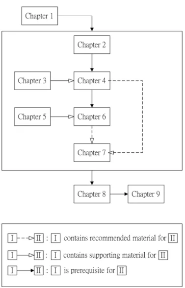
This study is divided into 9 chapters. Figure 1.1 shows the association between chap-ters. Chapter 2 gives a brief overview of Methadone Maintenance Therapy Data and literature reviews of research on the MMT. The data of the daily methadone dosages for 314 participants for a period of 180 days is selected. We propose a so-called category-ordered data in Section 2.4.1. The category-category-ordered data for 314 participants for 180 days is denoted by CO314, and will be used throughout this study.
In Chapter 3 we review clustering methods and dissimilarity functions.
In Chapter 4 we propose the p-dissimilarity. The p-dissimilarity is used to measure dissimilarity for data whose variables have characters of categorical and ordinal scales. Also, it can be used for incomplete data. The p-dissimilarity is based on the assump-tion that it is the neighbouring categories which contribute the most to distinguish the target category. The purpose of the assumption is to find clusters whose participants share similar dosage patterns in terms of sequences of categories. The p-dissimilarity involves two parameters. p is a switch between data being treated as categorical and ordinal andβ is for measuring dissimilarity when missing values occur.
In Chapter 5 we review indexes for the determination of the number of clusters, namely the Calinski and Harabasz (CH) (Calinski and Harabasz [1974]), the Average Silhouette Width (ASW) (Kaufman and Rousseeuw [1990]; Rousseeuw [1987]) and the Prediction Strength (PS) (Tibshirani et al. [2001]). The ASW and the PS are used in this study. We propose rules to modify the Prediction Strength in Section 5.3.1. Also, in order to avoid confusion, we call the equations for computing the dissimilarity between objects “functions” and those for determining the number of clusters “index”.
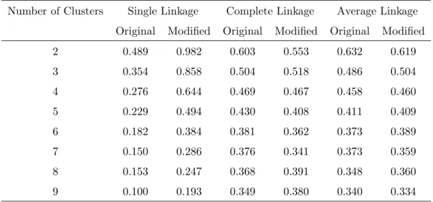
Chapter 6 begins by selecting the value for β, p and the clustering method. We apply the p-dissimilarity to CO314and compare the Single Linkage, the Complete Link-age, the Average Linkage and the PAM method by their values of the ASW and the modified PS. The values for the PAM method are higher and therefore the PAM method
is selected. In Section 6.2 we propose a null model test involving a null model and para-metric bootstrap (Efron and Tibshirani [1993]). The purpose is to investigate whether the clusters found according to the value of the index can be explained by random variation. The process of the null model test is as follows. A null model is constructed to represent a real data. But the null model has no structure of clusters, it is unknown whether there exist clusters in the real data. Then, the null model and boostrap are used to explore the distribution of a statistic such as values of the ASW. Next, the value of the ASW for the real data is compared with the distribution of the values for the null model. In Section 6.3 we show an application of the null model test to CO314. We use relative frequencies to describe the movements from categories to categories over time. Except for the category for missing dosages, we find that the dosage in categories following a valid prescription is stable and the movements between categories in ac-cordance with a weekly prescription. We then construct a Markov null model without structure of clusters, in which the distributions of the categories are the same as those of CO314. Five clusters are selected.
In Chapter 7 we propose two ordering algorithms for the heatplot in order to eval-uate the quality of the clustering. The algorithm of MDS is for general use and the algorithm of projection vectors is for the PAM method. We first use MDS to decide the location of clusters on a heatplot in order to preserve clusters. We then apply either the MDS method or projection vector method to order participants within a cluster. Also, the ordering algorithm of projections with the heatplot is used for a visual significance test.
In Chapter 8 we present a sensitivity analysis of clusters and list demographic data of the five clusters. Some conclusions are drawn in Chapter 9. Despite the fact that no significant clustering structure is observed, the sequences of categories for clusters are clinically useful to prescribe a proper dosage to increase the efficiency of methadone maintenance therapy.
Figure 1.1: Schematic representation of the organization of the contents of the thesis
-Methadone Maintenance
Therapy (MMT)
In this chapter a quick overview of the Methadone Maintenance Therapy (MMT) is given, followed by some research that has been carried out on it. Section 2.2 introduces the MMT database. The initial sample is composed of demographic details and the dataset of records of dosage taken. The study period is set to 180 days. For modelling daily methadone taken by participants for 180 days, a subset of 314 participants is selected from the initial sample (see Section 2.3). In Section 2.4.1 a new data format is created by transforming dosages into categories. The data consist of seven categories in which six categories have an ordinal scale for representing dosages and one category for missing dosages. We call it category-ordered data. The records of dosage taken for the 314 participants for 180 days is denoted by Dosage314. The category-ordered data for the 314 participants for 180 days is denoted by CO314. A heatmap plot is used to have an overview of the datasets. In this study, we perform a clustering analysis on CO314.
2.1
Literature review of methadone
Methadone was developed in 1934 to relieve pain. It was cheaper and less addictive. Later on, it was used as a heroin substitute in a treatment called Methadone Mainte-nance Therapy (MMT). In Taiwan, MMT was introduced in 2005. The main purpose
of MMT is to minimize the harm associated with heroin use (Ward et al. [1999]). The idea of MMT is to let drug users reduce the use of heroin by addicting to methadone and then quit the use of methadone. The effect of methadone lasts 24 hours and conse-quently it has to be taken on a daily basis. Ball and Ross [1991] reported, on average, a clinic received 1800 inquiries a year, but fewer than 200 people commenced MMT. In addition, only 38 percent of the 200 stayed in the therapy after a year. Also, par-ticipants who remained for more than six months had a marked drop in their drug abuse.
In some studies, the effectiveness of methadone maintenance was measured by mor-tality rates (Termorshuizen et al. [2005]), number of times illicit drugs (Marsch [1998]; Strain et al. [1993a,b]), frequency of criminal activity (Gossop et al. [2000]; Marsch [1998]; McLellan et al. [1985]; Powers and Anglin [1993]), cost (Masson et al. [2004]) etc. Research showed that methadone did indeed have a positive effect on drug users and on society.
More research has been done on daily methadone dosage taken by participants. Strain et al. [1993a] studied treatment retentions and illicit drugs use. They com-pared the groups of low to moderate doses of methadone and found that low dose of methadone (≤20 mg) may improve retention but were inadequate for suppressing illicit drug use. Langendam et al. [1998] regarded dosage greater than 60 mg as high. They observed that participants requested to stay at lower dosage because of fear of double addiction and of using drugs other than methadone. Bellin et al. [1999] studied associ-ations between criminal activity and methadone dosage. They found drug user on high dose (≥60 mg) were less likely to return to jail than those on low dose. Maxwell and Shinderman [2002] compared high dose participants (≥100 mg/day, mean 211 mg/day) with control participants (<100 mg/day, mean 65 mg/day). Their result showed that high dose was more effective in treating heroin addicts. While Maremmani et al. [2003] observed that many heroin addicts had positive outcomes with lower dosages. The basic issue of summarizing their studies is that they have different definitions for high dosage. To date there is no clear principle for the determination of the methadone dosage. However, if there were one, response to methadone could be significantly im-proved (Maremmani et al. [2003]; Maxwell and Shinderman [2002]).
There are more research on associations between types of methadone programmes and participants’ characteristics. Murray et al. [2008] considered methadone dosage and personality disorders. The American Psychiatric Association divided personality disorders into three groups. Cluster B was one of them. It included histrionic, narcis-sistic, antisocial and borderline personality disorders. Murray et al. [2008] surveyed 54 participants from a methadone maintenance clinic and found that methadone dosage might be uniquely related to the personality pathology. They suggested that methadone dosage might be a response to misery and physicians might need to communicate with heroin addicts with Cluster B pathology for methadone dosage to some extent. Peles et al. [2007] reported the major risk factors for depression were female gender and high dose (>120 mg). Pud et al. [2012] took account that participants in MMT frequently experienced pain, depression and sleep disorders. They attempted characterize clusters of MMT participants and studied the association between these clusters and quality of life measures. Participants were grouped into three clusters, one of which had highest severity levels of pain, depression and sleep disorders. This cluster scored lowest on all quality of life measures. Also, they reported pain was the most important symptom differentiating MMT patients. Gossop et al. [2000] studied patterns of improvement after receiving MMT for a year. They performed a one year follow-up study on 478 participants. They found that daily methadone dosage of participants who continued to use the drugs during the treatment had a large variation. They used the Euclidean distance K-Means clustering method to group the participants according to their fre-quency of illicit drug use, including opiates, stimulants and benzodiazepines. Four groups were identified. Two groups showed substantial reductions in their illicit drug use and criminality. They concluded that methadone dosage might be related to a cer-tain group and taking methadone might be of benefit to some groups. This suggested that it might be possible to develop a principle to prescribe the best dosage for certain subgroups whether dosage be high or low, which will help participants have positive outcome.
2.2
MMT database
An MMT project was launched by a hospital in central Taiwan. Due to concerns about confidentiality, the name of the hospital is not given here. The project provided an
opportunity to acquire more information about this therapy and offered the possibility of developing a principle to prescribe dosage by assessing patterns of daily methadone dosage administered to participants. As part of the MMT project, an MMT database was developed to manage the records of its participants. The MMT database sys-tem was a syssys-tem for storing the demographic details, medical history and methadone dosage records of participants. Firstly, the demographic details, which included age, gender, education, etc., were recorded when participants visited the hospital for the first time. Secondly, the medical history, which included the frequency of heroin use, urine drug tests, an HIV test, etc., was recorded when participants re-visited the hos-pital. However, not all of the participants underwent the urine drug tests and the HIV test. Thirdly, the methadone dosage records, which included records of prescription and records of dosage taken by participants, were recorded in two steps. (1) A participant visited a doctor and received a 7-day prescription. Subsequently, the system generated seven records, one record for each day of the prescription, with respect to the dosages shown on it. At the same time, the system generated seven zeroes for records of dosage taken. (2) In the following seven days, zeros would be changed to the actual dosage taken by participants every single day they visited the hospital.
Three datasets were recorded; however, they were not synchronized. There were cases where nurses accidently forgot to file participants’ data when they visited the hospital for the first time. As a result, these participants had no demographic de-tails. There were also cases where participants registered with doctors but failed to see their doctors. Consequently, they had no methadone dosage records. These kinds of mismatch happened quite often when merging several datasets. Another issue of this system was the process of recording daily methadone dosage. Seven zeroes for records of dosage taken were generated in advance. If participants did not go to the clinic to take methadone, their records remained zeroes. Later, we will discuss these zeros from an aspect of addictions should not be treated as zeroes.
2.2.1 Data for prescription and dosage taken
In this section we detail the difference between prescription and dosage taken in terms of restriction and daily record.
T able 2.1: Illustrati on of the data recording pro cess of a pa rticipan t o v er a p erio d of 8 da ys. -The table illustrates ho w prescriptions and dail y methadone dosage tak en of a participan t are re corded b y the MMT database in resp onse to ev en ts o v er a p erio d of 8 da ys. The tw o dosage records are recorded in tw o steps. (1) Sev en records of prescription are generated once a prescription is receiv ed. A t the same time, sev en zero es for records of dosage tak en corresp onding to the v alid dates of prescription are generated. (2) In the follo wing sev e n da ys, the zero records will b e changed to the actual d os age tak en b y the participan t. In the last column, RP represen ts the set of the records of the prescriptions dosage, while RD represen ts the se t of records of dosage tak en b y this participan t. Da y Ev en t Resp onse Database 1 Receiv e a 7-da y prescription of 50 mg T ak e 40 mg methadone Generate 7 prescription records Generate 7 zero records Change the 1 st zero to 40 mg RP= { 50, 50, 50, 50, 50, 50, 50 } RD= { 40, 0, 0, 0, 0, 0, 0 } 2 T ak e 45 mg methadone Change the 2 nd zero to 45 mg RP= { 50, 50, 50, 50, 50, 50, 50 } RD= { 40, 45, 0, 0, 0, 0, 0 } 3 F ail to tak e methadone Remained 0 mg RP= { 50, 50, 50, 50, 50, 50, 50 } RD= { 40, 45, 0, 0, 0, 0, 0 } 4 T ak e 50 mg methadone Change the 4 th zero to 50 mg RP= { 50, 50, 50, 50, 50, 50, 50 } RD= { 40, 45, 0, 50, 0, 0, 0 } 5 Receiv e a 7-da y prescription of 60 mg T ak e 55 mg methadone Generate 7 prescription records Generate 7 zero records Change one of the 5 th zeros to 55 mg RP= { 50, 50, 50, 50, (50,60), (50,60), (50,60), 60 } RD= { 40, 45, 0, 50, (55, 0), (0, 0), (0, 0), 0 } 6 T ak e 55 mg methadone Change one of the 6 th zeros to 55 mg RP= { 50, 50, 50, 50, (50,60), (50,60), (50,60), 60 } RD= { 40, 45, 0, 50, (55, 0), (55, 0), (0, 0), 0 } 7 T ak e 60 mg methadone Change one of the 7 th zeros to 60 mg RP= { 50, 50, 50, 50, (50,60), (50,60), (50,60), 60 } RD= { 40, 45, 0, 50, (55, 0), (55, 0), (60, 0), 0 } 8 T ak e 45 mg methadone Change the 8 th zero to 45 mg RP= { 50, 50, 50, 50, (50,60), (50,60), (50,60), 60 } RD= { 40, 45, 0, 50, (55, 0), (55, 0), (60, 0),45 }
There was no restriction on getting prescriptions, but participants were allowed to take methadone once per day. The prescription dosage was the maximum dosage that a participant could take in a day. The initial prescription dosage for the participants who had no experience of methadone was 20 mg. Then, doctors adjusted methadone dosage every seven days according to their subjective judgement and participants’ pref-erence of prescription dosage settings. In the MMT project, 10 mg was used as a unit of adjustment of prescription dosage in practice. However, addictions to heroin varied from participant to participant. Some participants might find that their unexpired prescriptions were not high enough to compensate the need for heroin, so they went to their doctors for new prescriptions with higher dosages. As a result, some participants had more than one prescription at the same time. To avoid participants overdosing, they were limited to use at most one prescription a day.
Only one of the multiple prescriptions was used on a day. Unfortunately, the sys-tem failed to indicate which one was used. Of these participants who had multiple prescriptions, they had more than one record of prescription but at most one nonzero record of dosage taken a day. In addition, values for those nonzero records varied from day to day. The variation of the values was a result for allowing participants to take a dose lower than what was indicated on their prescriptions. The reasons of this were as follows. Heroin users took MMT because of lack of money for drugs, court orders, determination of quitting drug etc. Some participants abused heroin while receiving the MMT, so they did not need a full prescribed dosage to accommodate their addi-tions. In contrast, some tried to reduce methadone dosage to defeat their addicaddi-tions. Therefore, each participant had at most one nonzero record of dosage taken a day and those nonzero records varied over time.
Table 2.1 illustrates the recording process of prescription and that of dosage taken of a participant over a period of 8 days since they first joined MMT. The first col-umn indicates the eight days. The second colcol-umn shows the explanation of events of getting prescriptions and taking dosage, while the third column shows the response of the recording system to the events. The last column shows the records of prescription, denoted by RP, and the records of dosage taken, denoted by RD. At the beginning, the participant in Table 2.1 visits their doctor and receives a prescription of 50 mg. Then,
this participant decides to take 40 mg methadone. Firstly, the system generates seven records of 50 for the prescription records and seven zeroes corresponding to the valid dates of their prescription. Once the participant takes 40 mg methadone, the first zero in DD is changed to 40. On day 2, 45 mg methadone is taken, so the second zero in DD is changed to 45. On day 3, no methadone is taken, so no change is made. On day 4, 50 mg methadone is taken, so the fourth zero is changed to 50. This participant has only one prescription from day 1 to day 4, but has multiple prescriptions from day 5 to day 7. On day 5, the participant visits their doctor for a new prescription before their current prescription expired. The new prescription is 60 mg. Seven records of prescription with a dose of 60 mg and seven zeros of records of dosage taken are gener-ated. As a result, the RP for day 5 is (50, 60). Later on, 55 mg methadone is taken, so the RD for day 5 is (55, 0). On days 6 and 7, 50 mg and 60 mg methadone are taken, respectively. Consequently, the records of dosage taken on day 6 and 7 are (50, 0) and (60, 0), respectively. Note that on days 5 to 7, the database dose not record which prescription is used. Based on limited information, our knowledge of record of dosage taken is that one of the zeros is changed. On day 8, the first prescription expires and 45 mg methadone is taken. The eighth zero is changed to 45.
Participants should have at most one nonzero record. Therefore, in later analysis, of those who had multiple records of dosage taken, the nonzero record would be considered first. For example, the records of dosage taken on day 5 were (0, 55) and it was 55 mg that would be used in the analysis.
2.3
Number of participants
Three datasets were collected from 1st January 2007 to 31st Dec 2008. However, they were not synchronized. The dataset of medical history showed that among those who took a blood test when they re-visited the hospital, 14 % took an HIV test. Also, 4914 urine drug tests were performed, 8 % of drug tests for morphine came positive and 1 % of drug tests for amphetamine came positive. Note that participants underwent more than one urine drug test. Some participants dropped and later returned to the treatment. Their demographic details were re-collected as participants who enter the MMT for their first time in practice. However, in our study, we appended their methadone records to
Figure 2.1: The number of participants over 732 days. - The x-axis is the date and the y-axis is the number of participants. This figure shows the number of participants that were found to have a record of dosage taken over the period between 1st January 2007 and 31st Dec 2008.
the existing dataset of dosages. With this dataset, Figure 2.1 shows the numbers of participants over time. As can be seen, at the beginning of the MMT project, there are only few people. Later on, the numbers of participants goes up as the hospital advertised MMT. Physicians considered participants who stayed in MMT more than six months as candidates being able to achieve abstinence. We limited participants to those who commenced MMT from 1st January 2007 to 30th June 2008 in order to ensure that participants should be able to stay in MMT for six months. A total of 1302 participants was selected. Twenty-one of them had only one nonzero record when they stayed in the MMT. They were eliminated in consideration of their non-contribution to form patterns of dosage taken. Taking into account their demographic details, a total of 1257 participants was obtained in which the two datasets could be matched. The initial sample was composed of demographic details and dataset of records of dosage taken.
2.3.1 Records of prescription and dosage taken for the initial sample
The records of prescriptions and records of dosage taken were stored separately. 1252 out of 1257 participants were found in the prescription dataset. A crucial issue of the records of prescription was that codings of prescription dosages were inconsistent. By coding, we meant the values that were used to indicate dosages. For instance, in the prescription dataset, 2 was used to indicate 10 mg, but 2 also referred to 20 mg.
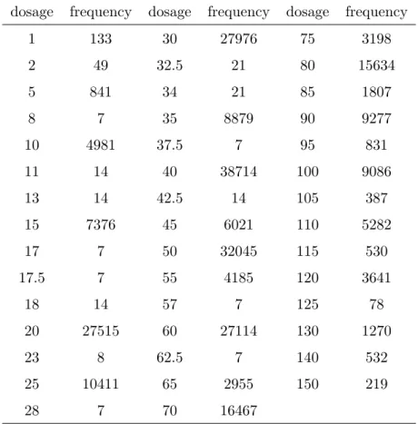
Table 2.2: Frequency of prescription dosage of the 1252 participants.- A total of 21465 prescriptions is selected. The first column refers to the coding in the records of prescription dosages. Unfortunately, we found that the codings referring to dosage are inconsistent. For example, a value 2 refers to 10 mg and it also refers to 20 mg. By and large, most physicians prescribe in intervals of 10 mg and some in intervals of 20 mg.
dosage frequency dosage frequency dosage frequency
1 133 30 27976 75 3198 2 49 32.5 21 80 15634 5 841 34 21 85 1807 8 7 35 8879 90 9277 10 4981 37.5 7 95 831 11 14 40 38714 100 9086 13 14 42.5 14 105 387 15 7376 45 6021 110 5282 17 7 50 32045 115 530 17.5 7 55 4185 120 3641 18 14 57 7 125 78 20 27515 60 27114 130 1270 23 8 62.5 7 140 532 25 10411 65 2955 150 219 28 7 70 16467
This kind of inconsistency happened when creating database without a complete cod-ing book in which a value that is unique to one dosage is listed. Regardless of the inconsistent codings, we attempted to have a better view of prescriptions by showing the frequency of prescribed dosage. This is shown in Table 2.2. Five dosages have their relative frequencies greater than 10%. They are 20 mg (12.20%), 30 mg (10.75%), 40 mg (14.93%), 50 mg (12.41%) and 60 mg (10.14%). Most physicians prescribe in intervals of 10 mg, some in intervals of 20 mg and some 5 mg.
All participants joined MMT on different dates and durations of their staying in MMT were different. Once participants joined MMT, days on which they took
Table 2.3: Number of participants of various attendance rates.-The attendance rates is the proportion of days of receiving methadone therapy to 180 days. Their corre-sponding numbers of participants are listed in the table.
Attendance rate (%) Maximum number of missing records Number of participants ≥90 18 169 ≥80 36 242 ≥70 54 314 ≥60 72 359 ≥50 90 412
methadone became important because the durations and days were the keys to form dosage patterns over time. So we attempted to create a picture to display the durations and days with/without taking methadone. Therefore, we defined a term “initial date”, denoted day 1, as referring to the first date on which the participants joined MMT. Figure 2.2 shows the information on durations and days for the 1257 participants. The x-axis represents the day and the y-axis represents the participant. The colour indi-cates whether participants took methadone. Black refers to nonzero records and white refers to missing dosages. The participants are ordered by the numbers of their nonzero records. Note that if the participants stay in the study, they should be able to provide at least 180 records of dosage taken. A reference line that indicates the 180th day is drawn. As can be seen, some participants have a chunk of missing records followed by nonzero records. This is because their drops out of and returns to MMT. A total of 1257 participants commenced MMT within dates ranging from 1st January 2007 to 30th June 2008, but only some of them provide nearly complete records for 180 days.
2.3.2 Selection of the meaningful sample
Ball and Ross [1991] reported, on average, only 38 percent of the participants stayed in the therapy after a year. A clustering result for the all 1257 participants will definitely give at least one group in which participants have most of their records appearing as missing dosages. Such a group has no contribution to the study at all. There-fore, instead of using 1257 participants, we should perform the analysis on a subset.
Figure 2.2: Records of dosage taken for the 1257 participants for 732 days. -The x-axis is the day and the y-axis is the participant. -The colour indicates where the missing value occurred, appearing in white. The participants are ordered by the numbers of their nonzero records. A vertical line at x=180 is drawn for the reason that the length of studying period was set at 180 days. Note that if the participants did not leave MMT, they should be able to provide at least 180 records of dosage taken.
This subset needs to be considered as a more purposeful sample for modelling daily methadone taken by participants.
The selection of such subset was done based on participants’ attendance to the clinic where they took methadone dosage. First of all, as six months was often used in MMT studies (Ball and Ross [1991]; Masson et al. [2004]), the length of the studying period was set to 180 days. Table 2.3 shows the number of missing records out of the 180 days and the number of participants for the attendance rates from 90% to 50%. At an attendance rate of 90 % or more, there are 169 participants who have at most 18 missing records. On the other hand, at a rate of 50 %, there are 412 participants who provide at least 90 records out of 180. The size of the former subset is too small and the proportion of missing records of the latter subset is slightly too high. Both of the two subsets are not good enough. As attendance rate goes down from 90 % to 80 %, an ad-ditional 73 participants are recruited. With another decrement in the attendance rate to 70 %, the number of participants goes up to 314. The expected maximum number of missing records is 54. For two participants whose 54 missing records are aligned on dif-ferent days, their dissimilarity would then depend on 180-54-54=72 records of observed dosages. However, at 60 %, the expected maximum number of missing records is 72. At the same situation, dissimilarity between two participants would then depend on at least 36 records of observed dosages. We assumed that 30% missing records would not affect the cluster analysis too much. Therefore, a total of 314 participants was used. The dataset of the records of dosage taken of the 314 participants over 180 days was denoted by Dosage314.
Of these 314 participants, 262 (83 %) were males and 52 (17 %) were females. Mean age at admission was 37± 7 years (range 23 to 60) and mean age of onset heroin was 25 ± 6 years (range 13 to 50). One hundred and fifty-six (50 %) participants had attended to high schools or universities. Seventy-seven participants were married or lived with a partner and 234 (75 %) participants were single or divorced. One hundred and ninety-nine (63 %) participants were occupied. Figure 2.3 shows the max, min, mean and mean±SD daily dosage records for Dosage314from day 1 to day 180. Mean dosage is 51 mg. As for these unselected 943 participants, mean age of commencing MMT was 36 ± 8 years (range 19 to 96) and mean age of onset heroin was 25 ± 7
Figure 2.3: The dosage taken records for 314 participants over 180 days.
years (range 11 to 57). Also, 760 (81 %) were males, 428 (45 %) received high school or higher education, 739 (78 %) were single or divorced, 591 (63 %) were occupied.
2.4
A new data format : category-ordered data
In our study, we observed that physicians thought categorically about prescriptions. From their point of view, prescribing a higher dosage meant that participants had their levels of methadone dosage moved from one to another. Such a movement should be, therefore, captured by categories. Moreover, prescription came with physicians’ assess-ments, a zero dosage should not be treated as zero, because participants’ addictions were not zero. Valid prescriptions meant that participants needed methadone to ac-commodate their addictions.
In the following sections, we introduce a so called category-ordered data. The category-ordered data for the 314 participants is denoted by CO314, the most important dataset that is used throughout this study. Then, we introduce imputation methods for the zero records of the category-ordered data. The imputed datasets are used to see the influence of missing values, which is evaluated by comparing the clustering result of CO314 and that of imputed datasets.
(a)
Figure 2.4: Number of prescriptions for the 313 participants over 180 days. - There are 313 out of 314 participants whose records could be found in the prescription dataset. This figure shows number of prescriptions over 180 days. The x-axis is the day and the y-axis is the participant. The colour represents the number of prescriptions. The max number of prescriptions on a single day for one participant is 4. The participants are ordered by the numbers of their nonzero prescription records.
2.4.1 Category-ordered data: CO314
Of these 314 participants in Dosage314, records of 313 participants are found in the prescription dataset. Figure 2.4 shows the number of prescriptions of the 313 par-ticipants over 180 days. The parpar-ticipants are ordered by their total of prescriptions in 180 days. As seen, participants occasionally have multiple prescriptions. In order to display the possible association between prescribed dosage and dosage taken, one participant is randomly selected from those who have only one prescription on every single day. Figure 2.5(a) shows the records of prescriptions and dosage taken of that participant from day 1 to day 180. The record of prescription dosage is indicated by circles, while record of dosage taken is indicated by crosses. The prescription dosage starts from an initial level of 20 mg/day, then there is an upward trend; moreover, it is a constant from day 29 to day 180 with a dosage of 70 mg. However, the records
(a) (b)
Figure 2.5: Records of prescriptions and dosage taken for two selected partici-pants from day 1 to day 180. - (a) shows a participant whose records of dosage taken fluctuates during the period of receiving prescriptions of 70 mg. (b) shows the records of another participant who also receives prescriptions of 70 mg; however, the records of dosage taken of this participant are more stable in comparison to those of the participant in (a).
of dosage taken fluctuate. This might be explained by the participant abusing drugs while receiving MMT. Next, in order to compare the records of dosage taken for two participants, a participant with a long sequence of prescriptions of 70 mg is selected. Figure 2.5(b) shows records of this participant. Following the same prescriptions of 70 mg, the records of dosage taken of these two participants are different.
There are two problems with Dosage314. Firstly, using methadone dosages to quan-tify additions, some degrees of dosage fluctuation are not meaningful. Failure to account for fluctuations which are caused by abusing illicit drugs might result in identifying false detoxification patterns. Therefore, given the same prescription with various dosage taken, participants should be considered as similar. However, there are participants with multiple prescriptions and there is no indication of which prescriptions were used. If no drugs are abused, methadone taken by participants should show long sequences of stability. Secondly, zero dosages need to be taken into account. Zero dosages mean participants did not show up for receiving methadone but not participants had no addictions. Zero dosages mean participants’ dosage taken records are missing. It is
reasonable to impute these missing dosages. However, from a medical point of view, a continuous 14 records of zero indicates that participants have left the study. Of those participants who are considered as having left the study temporarily, it is reasonable to impute their records by using the observed dosage. In contrast, of these who are considered as having left the study for good, the records should remain as they are. So, some missing dosages remain after imputation. But again, these records should not be treated as zeros. Also, the dissimilarity between a missing dosage and an observed dosage is not defined in most dissimilarity functions.
We attempted to construct a new data format by categorizing daily methadone dosage. The new data was used as a solution for the aforementioned issues. The purpose of categorizing dosage was to alleviate the impact caused by fluctuation, to consider participants with same prescriptions as similar, and to keep missing dosages. The missing dosages often occurred as a sequence. The pattern of missing dosages was of interest. In the new data, a participant who regularly took dosage in an interval was considered as having stable dosage. In contrast, changing to another interval regardless how far the movement meant that their dosage was moved to another dosage level. The advantages were as follows. The impaction of the fluctuations were minimized. It was not guaranteed that of these participants who used the same prescriptions, all were then regarded as similar; but, at least, most were considered as similar. Moreover, the missing dosages were categorized. By categorizing, we could define dissimilarity of missing dosages for distinguishing the missing dosages and observed dosages. Then, a dissimilarity-based clustering could be performed.
In order to categorize dosages, we needed cut points of dosages. Here are how the dosage levels were used in the research about methadone. In the research of Mattick et al. [2009], doses between 20 and 35 mg were classified as low dose, between 50 and 80 mg as medium dose and 120 mg or more as high dose. Johnson et al. [2000] used high dose (60 to 100 mg) and low dose (20 mg). In the research of D’Aunno and Pollack [2002], patients were classified into three groups by methadone dosage, less than 40, 60, and 80 mg. Although doses were often increased in 10 mg increments in MMT, the doses of 20, 60, 100 mg were most likely to be used to classify dosage levels in the
literature.
In our study, cut points for categorizing dosages were defined by the physician. He suggested that dosage in the range of 20 mg could be considered virtually the same. This meant that the qualitative difference between two dosages in the same interval could be treated as irrelevant. Therefore, observed dosages were transformed into sev-eral ordered sets, being intervals with the width of 20 mg, and the missing dosages were categorized, being represented by a category. The new data consisted of seven categories in which six categories had an ordinal scale for representing dosages and one category for missing dosages. The six categories represented for dosages smaller than or equal to 20 mg, 21-40 mg, 41-60 mg, 61-80 mg, 81-100 mg and greater than 100 mg. The new data was called “category-ordered data” throughout this study. The new dataset, denoted by CO314, was transformed from Dosage314.
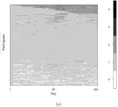
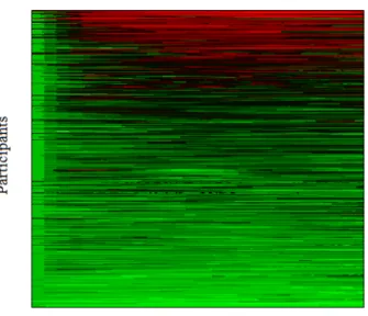
To explore the uncategorized dataset Dosage314and the categorized dataset CO314, a heatplot is used. It is a technique to represent data by color and each horizontal line in a heatplot represents data of each participant. However, locations of participants determine the efficiency of the heatplot in terms of displaying data with respect to a purpose. Research on ordering participants for increasing the efficiency of heatplots is carried out in Chapter 7 in which we use heatplots for viewing data and evaluating clustering results. Figure 2.6 shows the heatplot of Dosage314 and that of CO314. Each horizontal line represents records of a participant from day 1 to day 180. In the graph on the left, the 314 participants are ordered by the average of their dosages. In the graph on the right, the order of participants mirrors that on the left. Figure 2.6(b) shows the colour spectrum of dosage and that of category. The values of dosage, ranging from 1 to 140, appear in a sequence of green, black and red. The values of category, ranging from 1 to 6, appear in black, red, green, blue, cyan and purple. Note that the colour white represents for missing values and category 7. What can be observed is that most of dosage records in the first week are in category 1, as the initial prescription dosage for participants, most of which have no previous experience of the MMT, is 20 mg. Subsequently, the colours of dosage start to change, reflecting the fact that the doctors started adjusting the dosage. In the figure on the right, about one-third of the participants shows dosage below 40 mg, one-third shows dosage from 41 to 60 mg and
one-third shows dosage greater than 61 mg. Among those with dosage higher than 61 mg, only few of them takes dosage more than 100 mg. Besides, it can be seen that, of these movements from categories to categories, most of them move to the next nearest categories.
2.4.2 Imputation of the category-ordered data
In this section we attempt to impute the missing dosages. Three datasets are generated but it is CO314 being used throughout this study. We perform imputation because the missing values were all treated the same, being categorized to one category, but we are curious about the influence of the missing values on clustering results. In order to see how much difference it makes, we attempt to construct datasets with imputation. Then, they can be used to see the influence of having treated the missing values the same in CO314. The effect is evaluated by comparing the clustering result of CO314 and that of imputed dataset. Results for the comparison are shown in Section 8.2.
The length of the sequences of category 7, which represented missing values, de-termined whether participants temporarily left the study or not. A sequence with length less than 14 means that the participant temporarily left the study. Because they temporarily left, we attempted to construct a dataset with imputation only on these sequences of category 7 with length less than 14. Denote the value of category on dayiby ci, whereci ∈Θ ={1,2, . . . ,7}. The imputation method works as follows.
1. identifying the days having category 7.
2. labeling the each long sequence of the category 7.
3. distinguishing sequences to which imputation might apply. Sequences should have length less than 14.
4. identifying the closest known values of category of each of the sequences. The imputation will only be applied to the sequences in which its closest known values of category are the same.
In Step 2, let ψ={s1, s2, . . . , sa},a <180, be a collection of these sequences where
is meant the number of category 7 in the sequence.
In Step 3, for those sequences with length greater than or equal to 14, because par-ticipants are considered as having left the study in days on which the sequence occurred, there is no way to assign the category to which they belong. Therefore, these records remain category 7. Denote the selected sequences for which the lengthes smaller than 14 bysj ={ci, . . . , ci+nj−1}.
In Step 4, for each sequence found in Step 3, the two closest known values are the one before and the one after, that is,ci−1 and ci+nj. For the sequences of whichci−1 is
equal toci+nj, the records are replaced by the valueci−1. In contrast, for the remaining
sequences, because there is no clear decision about whether the category 7 should be replaced by a value close toci−1 or a value close to ci+nj, we decide to let the records
remain category 7.
Here is a