INTERACTIVE SOUND PROPAGATION FOR MASSIVE MULTI-USER AND DYNAMIC VIRTUAL ENVIRONMENTS
Micah Taylor
A dissertation submitted to the faculty of the University of North Carolina at Chapel Hill in partial fulfillment of the requirements for the degree of Doctor of Philosophy in the
Department of Computer Science.
Chapel Hill 2014 Approved by: Dinesh Manocha Gary Bishop Ming Lin Russ Taylor
©2014 Micah Taylor ALL RIGHTS RESERVED
ABSTRACT
Micah Taylor: Interactive Sound Propagation for Massive Multi-user and Dynamic Virtual Environments
(Under the direction of Dinesh Manocha)
Hearing is an important sense and it is known that rendering sound effects can enhance the level of immersion in virtual environments. Modeling sound waves is a complex problem, requiring vast computing resources to solve accurately. Prior methods are restricted to static scenes or limited acoustic effects. In this thesis, we present methods to improve the quality and performance of interactive geometric sound propagation in dynamic scenes and precomputation algorithms for acoustic propagation in enormous multi-user virtual environments.
We present a method for finding edge diffraction propagation paths on arbitrary 3D scenes for dynamic sources and receivers. Using this algorithm, we present a unified framework for interactive simulation of specular reflections, diffuse reflections, diffraction scattering, and reverberation effects. We also define a guidance algorithm for ray tracing that responds to dynamic environments and reorders queries to minimize simulation time. Our approach works well on modern GPUs and can achieve more than an order of magnitude performance improvement over prior methods.
Modern multi-user virtual environments support many types of client devices, and current phones and mobile devices may lack the resources to run acoustic simulations. To provide such devices the benefits of sound simulation, we have developed a precomputation algorithm that efficiently computes and stores acoustic data on a server in the cloud. Using novel algorithms, the server can render enhanced spatial audio in scenes spanning several square kilometers for hundreds of clients in realtime. Our method provides the benefits of immersive audio to collaborative telephony, video games, and multi-user virtual environments.
Dedicated to Christine, Charlotte, and Thomas.
ACKNOWLEDGEMENTS
I want to thank the members of my committee for their feedback and advice: Gary Bishop, Russ Taylor, and Nicolas Tsingos. I want to thank Dinesh Manocha, Ming Lin, and the members of the GAMMA group for all their support, criticism, and insight over the years. I have enjoyed working with all of you.
I especially want to thank Zhimin Ren, Qi Mo, and Lakulish Antani for their support. I also thank my colleagues at Rose-Hulman, who supported and trusted me during the last years of this work. Each of you helped me grow as a scientist and a friend.
There were many people who helped me see the joy in learning, long before I understood their generosity: James Frazier, Ken Holmes, Mark Ardis, and J. P. Mellor. My family back in Indiana also gave me tremendous support before and during this work; I cannot thank them enough for their love and encouragement.
I am very grateful for my friend Anish Chandak, without whom I would never have completed this work. I could always go to him for valuable advice and careful consideration, no matter the difficulty of the problems facing me.
Finally, I want to thank my lovely wife, Christine, for holding my hand during this adventure. Her endless love and wisdom led me to where I am today.
TABLE OF CONTENTS
LIST OF TABLES . . . xi
LIST OF FIGURES . . . xiii
1 INTRODUCTION. . . 1
1.1 Physical properties of sound . . . 1
1.2 Multi-user voice communication. . . 4
1.3 Information in sound . . . 5 1.4 Sound simulation. . . 6 1.4.1 Input. . . 7 1.4.2 Propagation. . . 8 1.4.3 Output. . . 9 1.5 Thesis statement . . . 9 1.6 Challenges. . . 10 1.7 Contributions . . . 11 1.7.1 Diffraction modeling . . . 12
1.7.2 RESound: unified propagation . . . 13
1.7.3 Guided visibility . . . 13
1.7.4 Rendering massive multi-user environments . . . 14
1.8 Organization. . . 15
2 RELATED WORK . . . 16
2.1 Sound synthesis. . . 16
2.2 Sound propagation . . . 17
2.2.1 Numerical solutions . . . 17
2.2.2 Geometrical methods. . . 18
2.2.2.1 Image source. . . 18
2.2.2.2 Accelerated image source methods . . . 19
2.2.2.3 Additional wave effects. . . 23
2.3 Audio rendering. . . 24 2.4 Voice communication . . . 26 3 FRUSTUM DIFFRACTION . . . 28 3.1 Algorithm . . . 28 3.1.1 Preprocess . . . 29 3.1.2 Edge containment . . . 31
3.1.3 Diffraction frustum construction. . . 32
3.1.4 Path generation. . . 33
3.1.5 Attenuation . . . 34
3.2 Accuracy . . . 34
3.2.1 Bell Lab Box comparison. . . 35
3.2.2 Accuracy of diffraction frustum . . . 37
3.3 Performance. . . 38
3.3.1 Diffraction cost and benefit . . . 38
4 RESOUND: A UNIFIED RAY FRAMEWORK. . . 40
4.1 System overview. . . 40
4.1.1 Acoustic modeling. . . 40
4.1.2 Ray-based path tracing. . . 42
4.1.3 RESound components . . . 43
4.2 Interactive sound propagation. . . 43
4.2.1 Specular paths. . . 44
4.2.3 Diffuse component . . . 46
4.3 Reverberation estimation . . . 47
4.4 Audio rendering. . . 48
4.4.1 Integration with sound propagation. . . 49
4.4.2 Issues with dynamic scenes . . . 51
4.4.3 3D sound rendering. . . 51
4.4.4 Adding late reverberation . . . 52
4.5 Performance. . . 52
4.6 Quality . . . 54
4.6.1 Quality . . . 54
4.6.2 Benefits. . . 56
5 GUIDED MULTIVIEW TRACING . . . 58
5.1 Guided propagation . . . 58
5.1.1 Ray traced propagation cost. . . 59
5.1.2 Guidance algorithm. . . 59
5.2 Multi-view GPU ray tracing . . . 62
5.2.1 GPU propagation. . . 63 5.2.2 Multi-view tracing. . . 65 5.2.3 Diffraction. . . 66 5.2.4 Path creation. . . 69 5.3 Audio processing. . . 70 5.3.1 Dynamic scenes. . . 70 5.3.2 Parameter interpolation. . . 71
5.3.3 Variable fractional delay. . . 72
5.4 Analysis. . . 73
5.4.1 Performance . . . 73
5.4.2 Audio processing limitations. . . 74
5.4.3 Comparisons. . . 75
6 RENDERING MASSIVE MULTI-USER ENVIRONMENTS. . . 79
6.1 Geometric acoustic similarity measure . . . 79
6.1.1 Distance . . . 80
6.1.2 Surface orientation . . . 81
6.1.3 Surface discontinuities. . . 82
6.1.4 Surface material. . . 83
6.1.5 Overall similarity measure . . . 84
6.2 Scene decomposition and sampling . . . 84
6.2.1 Similarity comparison . . . 84
6.2.2 Sample merging. . . 85
6.2.3 Acoustic regions. . . 86
6.2.4 Simulation of sound propagation. . . 88
6.3 Storage and reconstruction. . . 89
6.3.1 Response representation . . . 89
6.3.2 Storage data structures. . . 90
6.3.2.1 Storing acoustic data. . . 90
6.3.2.2 Efficient data indexing. . . 91
6.3.3 Response reconstruction and rendering . . . 93
6.4 Validation. . . 94
6.4.1 Error computation. . . 95
6.4.2 Similarity measure thresholds and validation. . . 96
6.4.3 Acoustic property error calculation. . . 96
6.4.4 Error map calculation. . . 98
6.4.5 Error analysis for reduction algorithms . . . 99
6.4.6 Metric analysis. . . 100
6.5.1 Similarity and reduction cost. . . 101
6.5.2 Precomputation: time and storage . . . 103
6.5.3 Runtime cost. . . 104 6.5.4 Comparison. . . 105 7 CONCLUSION . . . 107 7.1 Diffraction. . . 107 7.1.1 Limitations. . . 108 7.2 RESound . . . 109 7.2.1 Limitations. . . 109 7.3 Guided visibility . . . 109 7.3.1 Limitations. . . 110 7.4 Massive scenes. . . 111 7.4.1 Limitations. . . 111 7.5 Future work. . . 112 BIBLIOGRAPHY. . . 114 x
LIST OF TABLES
3.1 Time/accuracy cost: We compare various subdivision levels to a beam
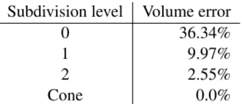
tracing solution on the Bell Lab Box. Our method . . . 37 3.2 Volume error: As the subdivision level increases, the error in the volume
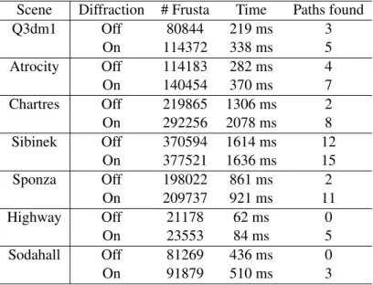
of the diffraction cone decreases . . . 38 3.3 Scene overview: Data on the scenes used for the performance results.
Some scenes are very open with much geometry visible from any given
point. Others are closed, with short visibility distances. . . 39 3.4 Diffraction benefit: Diffraction incurs a slight performance decrease, but
often finds more propagation paths. . . 39
4.1 Performance scaling: We show the performance scaling of our frustum
tracing and ray tracing implementations.. . . 53 4.2 Performance: Test scene details and the performance of the RESound components.. 53 4.3 Reverberation timings: The time cost to estimate the reverberation decay
is quite small compared to propagation times.. . . 54 4.4 Reverberation decay times Statistical predicted times compared to
RE-Sound measured times for two models.. . . 56
5.1 Performance in static scenes: The top two represent simple indoor and outdoor scenes. The third one is a well known acoustic benchmark and the fourth one is the model of Sibenik Cathedral. The number of reflections (R) and edge diffraction (D) are given in the second column. The time spent in computing propagation paths (on GPU) is shown in the PT column and audio processing (on CPU) is shown in the AT column. The simulation begins with 50k visibility samples; we measure the performance after 50
frames. . . 74 5.2 Performance per recursion: Average performance (in ms) of our
GPU-based path computation algorithm as a function of number of reflections performed. The Desert scene also includes edge diffraction. 50k visibility
samples were used.. . . 75
6.1 Example scenes: Physical sizes for the indoor and outdoor scenes are given in meters (m). The sample count is for a regular grid at the given
6.2 Precomputation time cost: Region segmentation using cube maps allows a significant reduction in precomputation time. The full grid data is generated based on the grid size given in Table 1 for each benchmark. Due to the high time and space cost, times marked with an * are based on
partial simulation. . . 103 6.3 Diffuse reflection cost: Diffuse reflections requires more simulation time
and slightly more storage space. Reduction results are for 75% node
reduction. . . 104 6.4 Storage cost: We compare storage cost of our reduction algorithm to
a full grid, both stored in our efficient sparse data structure.We observe significant improvement for large scenes. Due to the high time and space
cost, times marked with an * could not be computed. . . 104 6.5 Compression: We combine several algorithms to produce highly
com-pressed scenes . . . 104 6.6 Max realtime mixes per core: This table shows mixing costs for 500ms
of decay data per stream. The setup time includes data structure access and LOS traces. The realtime mixing step in our system is performed in
less than 20ms. . . 105 6.7 Comparison: We compare some features of our approach with other
precomputation methods, including PART [Siltanen et al., 2009], Wave-grid [Raghuvanshi et al., 2010], IS gradient [Tsingos, 2009], DP Cache
[Foale and Vamplew, 2007], and Reverb graph [Stavrakis et al., 2008]. . . 106
LIST OF FIGURES
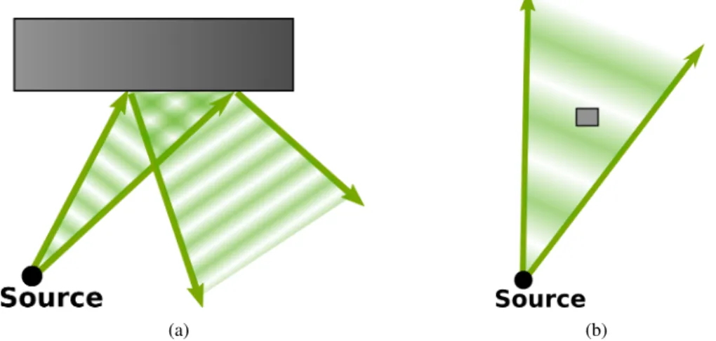
1.1 Wavelength and object size: Objects and details much larger than the wavelength (a) cause the wave to reflect in a specular manner, while objects
much smaller than the wavelength (b) have little influence on the wave.. . . 2 1.2 Diffraction: Edge diffraction occurs when a wave encounters an object
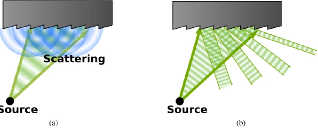
edge and some of the wave propagates in the shadow region. . . 3 1.3 Wave scattering: Diffuse reflections (a) are a result of many diffraction
interactions when surface details match wavelength; if wavelength is much
smaller than the details (b) specular reflection occurs.. . . 3
2.1 Image source: From the Source, image sources SAand SBare created
over walls A and B respectively. Only SAis occlusion free; a reflection
sequence using SBis physically impossible.. . . 19
2.2 Receiver size: For the subset of first order reflection rays shown, smaller receivers (a) result in fewer visibility samples needing to be culled, but may have aliasing artifacts if the scene changes slightly. Larger receivers (b) will have more sequences that must be validated and discarded, but
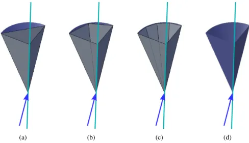
fewer aliasing artifacts. . . 21 2.3 Adaptive Frustum Tracing [Chandak et al., 2008]: Adaptive Frustum
Tracing traces frusta primitive from the source S (a). As subdivision
increases (b,c), frustum tracing approaches the ideal solution (d). . . 22
3.1 Overview of our edge diffraction algorithm: Possible diffracting edges are detected and marked as a preprocess. During the simulation, frusta are checked for diffracting edge containment. If so, a new diffraction frustum is created. After the propagation is complete, the diffraction paths are
attenuated by the UTD coefficients. . . 29 3.2 Preprocessed edge types: (a) Planar edges that never diffract; (b) exterior
edges that always diffract; (c) interior edges and (d) disconnected edges
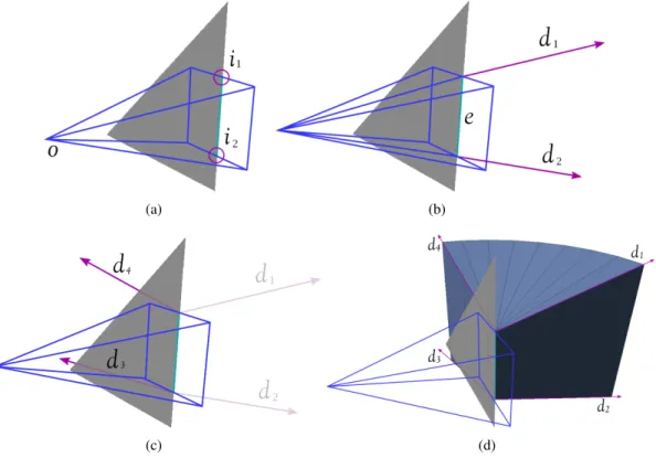
that can be configured by user choice to diffract. . . 30 3.3 Diffraction frustum creation: (a) Given a frustum’s origin o and its edge
intersection points i1and i2, (b) the edge axis e and the initial diffraction
vectors d1and d2are created. (c) Rotating d1and d2about the edge axis
towards the far side of the diffracting wedge sweeps a diffraction cone in the shadow region bounded by the final vectors d3and d4. (d) We create
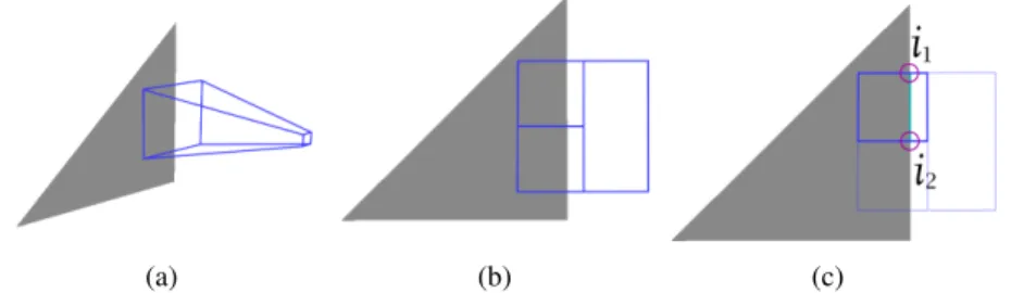
3.4 Edge containment check: After the frustum encounters a triangle (a), its face is projected into the triangle plane (b). Each diffracting edge is then checked for intersection with the face (c) to find the intersection points i1
and i2.. . . 31
3.5 UTD attenuation: A radio is playing behind the door. The light green region shows the spectrum for the direct path when the door is open. The dark green region shows the spectrum of strongest diffraction path as the
door closes.. . . 34 3.6 Bell Lab Box [Tsingos et al., 2002]: The Bell Lab Box is a simple room
divided by a diffracting baffle. The image shows the 45 paths resulting
from two orders of specular reflection and one order of diffraction. . . 35 3.7 Path length: As subdivision level increases, more paths are found and
the error decreases.. . . 36 3.8 Frustum subdivision accuracy: the resulting diffraction cone with a
subdivision of 0 (a), subdivision of 1 (b), and subdivision of 2 (c). The
diffraction frustum approximates the ideal cone (d).. . . 37 3.9 Evaluation scenes: (a) Q3dm1, (b) Atrocity, (c) Chartres, (d) Sibinek,
(e) Sponza, (f) Highway, (g) Sodahall.. . . 38
4.1 The main components of RESound: scene preprocessing; geometric propagation for specular, diffuse, and diffraction components; estimation
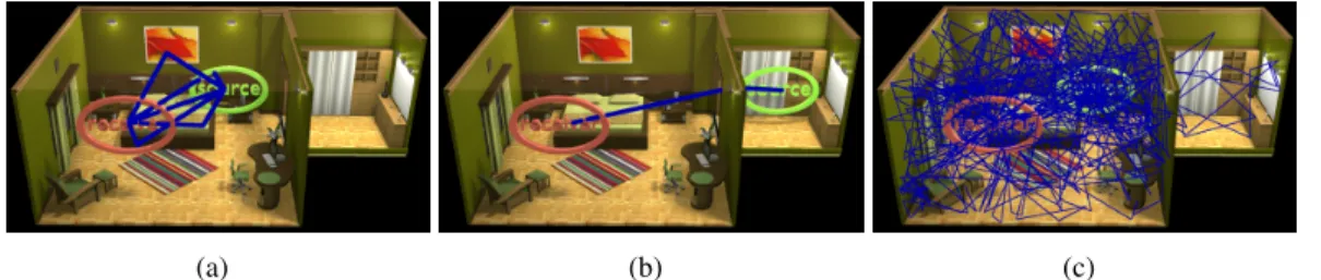
of reverberation from impulse response; and final audio rendering.. . . 41 4.2 Example propagation paths: This scene shows (a) specular, (b)
diffrac-tion, and (c) diffuse propagation paths. . . 41 4.3 Unified ray engine: Both (a) frustum tracing and (b) ray tracing share a
similar rendering pipeline.. . . 45 4.4 Extrapolating the IR to estimate late reverberation: The red curve is
obtained from a least-squares fit (in log-space) of the energy IR. The green
vertical line is the RT60 mark where the signal has decayed by 60 dB. . . 48 4.5 Algorithm overview: An overview of the integration of audio rendering
system with the sound propagation engine. Sound propagation engine updates the computed paths in a thread safe buffer. The direct path and first order reflection paths are updated at higher frequency. The audio rendering system queries the buffer and performs 3D audio for direct and first order paths and convolution for higher order paths. The cross-fading
and interpolation components smooth the final audio output signal. . . 49 4.6 IR convolution: The input audio signal S is band passed into N octave
bands which are convolved with the IR of the corresponding band.. . . 50 4.7 Test scenes used: (a) Room, (b) Conference, (c) Sibenik, and (d) Sponza. . . 53
4.8 Specular paths: With a subdivision (a) level of 2, frustum tracing finds 13 paths. A subdivision (b) level of 5 finds 40 paths. The (c) image-source
solution has 44 paths.. . . 54 4.9 Diffraction paths: Increasing the frustum subdivision improves the
diffrac-tion accuracy. . . 55 4.10 Path direction: From source S to listener L: (a) The simple direct path is
physically impossible, but (b) diffraction and (c) reflection paths direct the
listener as physically expected.. . . 57
5.1 Sample-based visibility: Visibility rays are traced from source S into the scene. Paths that strike receiver R are then validated. (a) A small receiver requires dense visibility sampling to find the propagation path. (b) Using a larger receiver allows sparse sampling resulting in fewer visibility tests,
however more validation tests are need to remove invalid path sequences. . . 60 5.2 Propagation test count: With a goal of finding 90% of the total paths
in the scene, an increasing number of visibility rays are traced and the minimum required size of the receiver sphere changes accordingly. With sparse visibility sampling, a large sphere is required, resulting in many validation tests. With dense sampling, the sphere size can be reduced. For specific cost values for visibility and path validation tests, some minimal
total cost exists.. . . 61 5.3 Guiding state machine: This state machine tracks the number of unique
contribution paths found. Solid lines are followed if the current path count matches the recorded maximum count, dashed lines are followed if the path count is less than the recorded maximum. States marked R+ and S+ increase the ray count and sphere size, while states marked R− and S− decrease the ray count and sphere size, respectively. At the Restart state, the maximum paths count is set to the current count. The (R+, S+) states attempt to recover lost paths before recording a new count. The main top
and bottom arms focus on reducing rays and receiver size respectively.. . . 62 5.4 Implementation overview: All scene processing and propagation takes
place on the GPU: hierarchy construction, visibility computations, specular and edge diffraction. The sound paths computed using GPU processing are returned to the host for guidance analysis and audio processing. The
guidance results are used to direct the next propagation cycle. . . 63 5.5 Multiview tracing: (a) From the source, rays are grouped into packets
that can be efficiently processed on the vector units. (b) However, a single packet may hit multiple surfaces, resulting in reflection packets that are
inefficient. (c) We reorder packets so that each reflection view can be traced efficiently. 64 5.6 Multiview performance: Multi-view ray tracing out performs standard
ray tracing for scenes (80k triangle scene shown) with many specular views.
5.7 Barycentric diffraction hit points: Using the barycentric coordinates of
a ray hitpoint, a diffraction origin d can be found on the triangle edge. . . 68 5.8 Edge diffraction: (a) Rays near the edge are detected for resampling. (b)
Diffraction samples are cast through the shadow region, bounded by the
adjacent triangle.. . . 68 5.9 Interpolation schemes: Different attenuation schemes applied for
attenu-ation interpolattenu-ation. Discontinuity in attenuattenu-ation between two audio frames interpolated with linear interpolation and Blackman-Harris interpolation. Delay interpolation is performed using a linear interpolation. Variable fractional delays due to linear delay interpolation are handled by applying low order Lagrange fractional delay filter on a supersampled input audio
signal during the audio processing step. . . 70 5.10 Fractional delay: Applying fractional delay filter and supersampling
input signal to get accurate Doppler effect for a sound source (2 KHz sine wave) moving away from the receiver at 20 m/s. The sampling rate of the input audio is 8 KHz. The supersampling factors are 4x and 8x for left and
right figures respectively. Zeroth order and third order Lagrange filters are applied.. . 72 5.11 Example scenes: The scenes used to test the performance of our
imple-mentation: (a) Music hall model; (b) Sibenik cathedral; (c) Indoor scene; (d) desert scene. While the music hall scene is not often used for low order acoustic simulation, we selected it to show the animation sequence in Figure 5.13. Sibenik cathedral was selected as a very challenging visibility
test case.. . . 73 5.12 Recursion path count: These figures show the number of paths found for
varying visibility rays. The receiver size is fixed at 1 meter. As visibility ray count increases, low triangle count scenes like the Music hall (a) are quickly saturated. However, in complex scenes like Sibenik cathedral (b),
higher visibility ray counts are required to explore the scene. . . 75 5.13 Music Hall animation: This figure compares various receiver size models
to our guided method. During frames 100-199, the source moves to a new position; during frames 300-399, the receiver moves to a new position. The top charts show the accuracy and the time cost over the animation sequence. The three middle charts show number of validation and visibility tests conducted by our guided method, in addition to the radius of the receiver. The bottom charts show the impulse response of our method compared to an accurate image source simulation for frames 50, 150, and 250. Our method is more accurate than the others, while incurring a small
additional time cost.. . . 76
6.1 Sample signature for FPS scene in Figure 6.8(b): The components of the similarity measure: (a) distance with black being near and white far, (b) direction with vectors shown as RGB components, (c) discontinuities in depth and direction, and (d) materials with three frequency bands shown
in RGB components. . . 80 6.2 Surface distance: The first-order propagation distance p is directly related
to nearby reflectors. v is the direct path to the receiver. fsrepresents the
shortest first-order reflection path as φsgoes to 0. f`represents the longest
first-order reflection path as φ`goes to π. Our algorithm measures the f
terms of p. . . 81 6.3 Surface orientation: Reflection direction r varies as a property of the
incoming vector v and the surface normal orientation n.. . . 82 6.4 Adaptive sampling: (a) Regular grid sampling creates a very high number
of samples; (b) we remove redundant samples; (c) adaptive sampling of
the scene with fewer samples.. . . 85 6.5 Data insertion: The decay data A, B, C is appended to a linked list and
the length of the list is the data index. The index is stored with a pointer to the decay data as a pair in a map. The index is paired with a position hash and stored in a hash table. The insertion can be performed in average O(log n) time. After all the data is stored, the linked list is converted to a linear array, for a total time complexity of O(n) and average storage cost
of O(n). . . 90 6.6 Data access: For runtime access, the query position is hashed and the
decay index is found in average O(1) time. The data array is then queried
for the final decay data. . . 92 6.7 Early response attenuation: The early response pressure is attenuated
for source/receiver pairs in the same region. . . 93 6.8 Example scenes: Our algorithm can generate environmental acoustic
effects in large virtual worlds and games. We show different benchmarks with their dimensions in meters: (a) simple outdoor scene (33 × 33 × 10); (b) first person shooter (FPS) game scene (30 × 60 × 20); (c) city scene (600 × 980 × 33); (d) canyon model (4000 × 4000 × 100). Our approach scales with the size of these models and can handle a large number of
sources and receivers in multi-player enviroments at interactive rates. . . 94 6.9 Sampling accuracy vs. error and cost: Naive subsampling (a) is the
most common way of reducing time and storage cost. As the threshold error in our adaptive sampling algorithm changes (b), the overall error in the acoustic evaluation metrics increases, while overall storage, pre-computation time, and number of samples decrease (FPS game scene).
6.10 Error maps: We compute acoustic evaluation properties in the FPS scene for (a) full dataset and (b) our reduced dataset. The details of these datasets are given in Table 6.2. The difference between these datasets represents the error in our solution (c). The total energy values for the source position
outlined in green are shown. . . 99 6.11 Segmentation error: The segmentation map for the FPS scene is shown
in (a), where each unique color is an acoustic region. The total energy relative error resulting from this segmentation is shown in (b) We show the source position sampled in Figure 6.10 as a green circle. The legend
for (b) is the same as the legend in Figure 6.12. . . 100 6.12 Error maps: We compute the relative error in FPS scene with respect to
different evaluation metric: (a) onset delay; (b) onset wave direction; (c) RT60; (d) and definition D. A wireframe of the scene is overlaid on the error maps. Red areas indicate high error. In most regions the errors in terms of onset delay, RT60 and definition are low. A few locations result
in high values of the onset direction relative error.. . . 101 6.13 Error values for different reduction algorithms corresponding to
dif-ferent acoustic evaluation metrics: The (a) adaptive algorithm performs better than any other; the other node placement algorithms guided by our signature, (b) flood fill and (c) sorted merge, perform much better than naive (d) subsampling. These error plots demonstrate the benefit of using our geometric acoustic similarity criteria along with the adaptive scheme as compared to other approaches. For example, the error reduction over sub-sampling algorithms can be large, as compared to that over flood-fill and single sort reduction. Due to high compute cost, these results only
include specular and diffraction responses. . . 102 6.14 Individual metric results: We show the reduction results when only a
single metric is enabled on the Small City scene. The chart title indicates which metrics are enabled with a 0 or 1: distance (d), direction (r), dif-fuseness (f), and material (m). The top row shows the results with all metrics enabled and the results from naive subsampling. The vertical axis is maximum error of any measured acoustic property, while the horizontal axis is the nodes remaining from the original count. Due to high compute
cost, these results only include specular and diffraction responses. . . 103
CHAPTER 1: INTRODUCTION
Our ability to hear sound waves is one of our most important senses. Along with sight, it is the only sense that can detect remote objects with high-fidelity [Blauert,1997]. Unlike sight, our hearing is not limited to a small field of view in front of us; hearing allows us to sense the world in any direction. Without turning to direct our focus, our sense of hearing can distinguish sounds that come from in front from those that come form behind. Our ability to emit sound complements our hearing, allowing communication through sound. Interaction with sound waves is shared by all humans and other animals. As a society, we have invested a great deal of effort in harnessing sound for communication and entertainment.
Like all waves, sound has complicated interactions with the environment. Sound waves begin at some vibrating source and propagate out through a medium. The waves may reflect and scatter as they encounter objects in the medium. These interactions alter the wave in ways that are understood. Our perception of sound is adapted to recognizing these changes in the wave, and we can derive information about the source and environment from the modified wave patterns.
1.1 Physical properties of sound
Sound begins as a mechanical vibration (itself a wave) of an object. The vibrations may be transmitted into the object’s containing medium and longitudinal waves propagate forth [Kinsler et al.,1999]. These waves are compressions and rarefactions of the medium.
The waves may vary in amplitude and frequency; our ears can perceive and distinguish both. The source of the mechanical vibration determines the wave properties. A high frequency vibration results in a high frequency wave. As the vibration is transmitted to the medium, the medium directly influences the speed of the wave, and consequently, its wavelength.
reflections result in the echoes heard in canyons or large empty rooms. The wave may also transfer some of its energy when it encounters objects, causing the object to vibrate. The object’s vibration may cause another sound wave to propagate. This is how sound travels through apartment walls. Some of these wave effects vary based on the wavelength of the wave. Since wavelength and frequency have an inverse relationship with wave speed, throughout the text we will often use wavelength and frequency interchangeably.
(a) (b)
Figure 1.1: Wavelength and object size: Objects and details much larger than the wavelength (a) cause the wave to reflect in a specular manner, while objects much smaller than the wavelength (b) have little influence on the wave.
If the object’s surface is smooth relative to the wavelength, the wave can be reflected specularly (Figure1.1a). This kind of reflection is similar to how light reflects in a mirror: the angle of incidence to the surface is the same as the exit angle for any portion of the wavefront. Similarly, if the entire object is much smaller than the wavelength, the wave continues propagation with change (Figure 1.1b).
However, for objects that have details that are similar in scale to the wavelength size, diffraction occurs (Figure1.2). For example, when a wave encounters an edge, some of the energy in the wave bends around the edge. Since the bending is related to wavelength, some frequencies may bend more than others. This can lead to audible sounds even when the sound source is out of sight of receiver. This is an important effect for humans, since it allows us to detect sound sources even when they are visually occluded.
If the object’s surface has surface complexity in similar scale to the wavelength of the sound wave, diffraction occurs due to the surface complexity and the resulting wave is scatters in a complex
Figure 1.2: Diffraction: Edge diffraction occurs when a wave encounters an object edge and some of the wave propagates in the shadow region.
(a) (b)
Figure 1.3: Wave scattering: Diffuse reflections (a) are a result of many diffraction interactions when surface details match wavelength; if wavelength is much smaller than the details (b) specular reflection occurs.
pattern (Figure1.3a). This interaction reflects the wave in a diffuse manner; the exit angle has a complex relationship to the incident angle. However, if the surface complexity is much larger than the wavelength of the sound wave, the wave reflects specularly off the individual surface facets (Figure1.3b).
As the wave moves through the environment, some energy is lost due to propagation through the medium. Additionally, each encounter with an object or medium change alters the waveform and may absorb energy. Since the speed of sound is hundreds of meters per second and typical indoor spaces are only a few meters big, the wave may undergo hundreds of interactions in just a few seconds. As the wavefront scatters, different portions are scattered and reflected along different paths through the environment, causing the wave’s energy to be spread out over time and frequency, and the wave amplitude to vary.
Eventually, some portion of the wave energy may arrive at a receiver. Human ears have organs that can sense the wave as changes in pressure. The changes in pressure in our ear canal are transmitted to our brain as neural signals, which are perceived as sounds. Since our ears are asymmetrical in the horizontal plane and the vertical plane, waves arriving from different directions diffract around our bodies in unique ways. Additionally, the wave must diffract around the head to reach both ears. This can delay the arrival of sound to one ear. All of these properties allow our brains to localize the sound source, that is, determine the approximate direction of the source.
1.2 Multi-user voice communication
Sound has been subject to much use and investigation over the centuries. Speech, the act of emitting purposeful sounds, is humanity’s fundamental method of communication.
As science established the properties of sound waves, humans have sought to harness sound for our advancement. Telephones and recording tools are the most obvious recent advancements. The invention of the telephone was humanities first tool that allowed natural two-way communication over vast distances. Telephones leverage our already existing biological tools in a natural way, unlike any technology heretofore.
Our technology continues to advance and humanity’s knowledge is now stored in more permanent and convenient written form. Even so, audio communication remains important, as written storage requires training and tools to use. Indeed, audio communication is so basic, that realtime voice communication between any two places in the world is almost taken for granted.
With the advent of the Internet, voice communication became extremely affordable and reliable. The flexibility of modern computers has allowed voice communication over vast distances to be trivially accessible and collaboration between large groups easily attained. Voice over Internet Protocol (VoIP) is the process of using the internet to enable voice communication. Voice data is recorded and compressed on one computer, then transmitted to a remote computer for reconstruction. The remote system attempts to recreate the input sound using rendering software and an output speaker system.
In modern VoIP systems, many people may be communicating in a single conversation. Since each person wishes to hear all other speakers, all voice data must be streamed to each client computer.
A peer-to-peer arrangement is when each clients sends all recorded voice data to each other client, but this may require significant network resources. An alternative is a client-server arrangement, where the voice data is sent to an intermediary, which aggregates the data and sends the result to each client. This moves the network and compute burden to the intermediary server.
1.3 Information in sound
Given the physical properties of sound waves and the way humans use sound to communicate, it is clear that waves can carry explicit information from their source as well as implicit information due to their propagation. From birth, our sense of hearing continually saturates us in sound information and our brains adapt to what we hear. We grow to be able to infer a great deal from the sounds that we hear and become naturally trained at coupling hearing with our other senses.
As discussed in Section1.1, human ears allow localization of sound sources. There is also a discrepancy between the perceptions of sight and sound. We spend most of our lives in an air medium where light travels very quickly and sound relatively slowly. We learn to recognize that when an accompanying sound response is delayed from a visual response, that the action that propagated the light and sound wave is some distance away. Children use this to determine the distance of thunderstorms by counting the seconds between a lightning strike and the corresponding thunder sound. Relative to our perception, light travels practically instantaneously, while sound travels at approximately 343 meters per second. Thus, every three seconds between lightning strike and thunder indicates that the storm is one kilometer away.
Each reflection of the sound wave sends energy along a new path through the environment. Some sound energy may arrive at the receiver along a path with no reflections, and is only delayed by the distance between source and receiver based on the speed of sound. Other energy arrives by way of several reflections. This energy must travel a greater distance and more energy is lost to the medium and the reflection, and is thus delayed with a lower amplitude. This results in echoes and reverberation. Humans come to expect sounds in large enclosed spaces to produce such reflected effects. Additionally, we can infer the size of the enclosed space based on the density and length of the echoes and reverberation. Cathedrals and canyons will have lots of echo and reverberations, living rooms will not.
Since we hear sounds our entire lives, we come to expect certain actions to have certain sounds. If the sound source is well known, we can detect changes in frequency and amplitude from the expected sound. Someone speaking from around a corner will be slightly muffled; music heard through a wall will be very muffled; a voice from far away will be quieter. The effect of the environment on the wave conveys information about the environment and the location of the source to us.
1.4 Sound simulation
Given how pervasive sound is in the physical world, it is desirable to be able to simulate the properties of sound. It is convenient to divide sound simulation into three parts: input, propagation, and output. Each part can be combined with others to form a complete sound rendering pipeline.
There are many applications for sound simulation. Architectural acoustics is the study of sound in man-made structures. Buildings have been designed with acoustics in mind for centuries. Many modern auditoriums have been built without regard to acoustic properties and suffer from intelligibility issues for both speech and music. Acoustic simulations can provide valuable insight into acoustic problems with existing structures as well as guide design of future structures . The propagation of sound waves through the architectural environment is the most important process that is modeled for this application. Most commercial acoustic simulators, such as CATT1, EASE2, and
ODEON3, are designed for architectural acoustics.
Many entertainment mediums rely on high quality visuals and audio. In film, Foley artists have long designed the sound effects that accompany on screen actions. Various physical objects are used to create artificial sounds that are expected by viewers, for example banging coconuts for horse foot steps. Many film visual effects are simulated in virtual environments for cost and safety reasons. It is reasonable that sound simulation could assist Foley artists in the creation of sound. For this application, the creation of sounds by physical contact would be important to simulate.
Video games are another medium that could benefit from sound simulation. Just as with film, three types of simulation could be useful: sound synthesis from contacts, sound propagation through environments, and sound output from speakers. An additional requirement is that all these simulations
1http://www.catt.se
2http://ease.afmg.eu
3
http://odeon.dk
must run interactively meaning that the simulation must match the visual simulation, often within a few milliseconds. Many games feature highly dynamic environments, where doors open and close, buildings collapse, and vehicles move around. The acoustic simulation must be able to respond to these dynamic events.
Virtual training simulations are interactive virtual environments similar to video games, but with clearly defined goals of enhancing the participant’s ability in specific areas. Possible simulations could be street crossings for blind people, battle training for soldiers, and emergency situations for medical personal. These applications require interactive and realistic visual and audio simulations to avoid the possibility of negative training.
Multimodal visualization is the use of several senses to convey data relationships. Visual displays are the most common way to visualize data, but sound can be used also. Voice communication systems with many participants can place each participant in a virtual auditory space to allow the listener’s natural localization to determine which participant is speaking. Simple auditory displays include how many operating systems alert users when long operations complete with an audible alert (a ’ding’ or such). In more realistic virtual environments, non-physical auditory cues can aid the participant in understand the virtual environment. With realistic propagation simulations, a participant could be alerted to activity in other parts of the virtual environment. Simplified versions of this exist in some video games in the form of ’map pings’ where an audible noise is made to draw attention to the environment. Auditory displays are not restricted to virtual environments.
Simulations can also be used to design better transmitters and receivers for very complex audio problems such as medical ultrasounds and underwater sonars. These require propagation simulations to account varying media in addition to the effects described above. Density changes result in changes in the speed of sound and make predicting wave propagation difficult.
1.4.1 Input
All sound simulations begin with some input sound signal. This can come from a recording of a real-world sound or synthesized using a simulation. Most common input sounds come from physical vibrations of materials in the environment captured with a recording device. Without careful planning, the specific radiation pattern of the physical event is not captured. Indeed, most recordings capture a single sound channel and this is insufficient to fully represent the input signal in a virtual environment.
A beamforming technique can use an array of recording devices to measure the radiation field more accurately.
An alternative to measuring physical sounds is to create the sounds synthetically. Sound synthesis is the process of creating sound signals algorithmically. Frequency modulations uses combinations of pure tones to form useful signals for music. Physical contact sounds can also be modeled by simulating material vibrations in contacting virtual objects.
1.4.2 Propagation
Once a sound wave is transferred to the environment’s medium, it begins propagating through the environment. Simulate of wave propagation must balance accuracy and speed. Humans can perceive a wide range of frequencies: 20 hertz to 20 kilohertz. With a typical speed of 343 meters per second in air, sound waves have a wavelength in the range of 17 meters to 1.7 centimeters. Most objects built and used by humans (furniture, office doors, cups, etc.) have similar scale to sound waves. This means sound has wave-like interactions with these objects. An acoustic wave equation predicts the propagation of sound waves. The details of this are discussed in Section2.2.
For visual simulations of light propagation, most wave effects can be ignored since the wave-length of light is on the order of hundreds of nanometers and wave effects on that scale are hard for humans to observe visually. Moreover, light travels much faster than sound, so only the steady state needs to be computed. Most light simulations model the light wave as a wave front of particles and ignore the time component.
Sound simulation is much more challenging as compared to visual simulation. Wave effects, like diffraction and interference are prominent and easily audible to humans. Sound also travels much slower and humans can easily detect delays, echoes, and reverberation effects caused by interactions from the environment.
Accurate simulations should be able to compute a wide range of frequency inputs and outputs, handle wave effects, and output correct time domain values. Solving all of these effects in a single simulation is difficult. The acoustic wave equation predicts all these effects, but is very time consuming to solve, as it scales with the fourth power of the maximum simulation frequency. Dynamic scenes further complicate simulation, since objects may shift during the simulation step
and frequency shifts from the Doppler effect are audible. Another consideration is environments where the medium density varies and the medium is in motion, such as atmosphere or ocean currents.
1.4.3 Output
Synthesis and propagation simulations are of no use without a means to render audible sounds for the listener. Since humans can hear frequencies up to 20 kilohertz, accurately reconstructing sound signals requires sampling rate of about 40 kilohertz, due to the Nyquist limit. Humans can perceive a wide range of amplitudes, from approximately one ten-thousandth of a pascal of pressure to tens of pascals of pressure.
Further complicating matters is the fact that sound waves arrive at a receiver from some direction, allowing the receiver to spatialize the source direction. Humans can spatialize in three dimensions since our ears are asymmetrical vertically and horizontally. The asymmetrical shape means that a wave will scatter differently based on arrival direction. This effect requires at least two output channels for realistic spatialization cues to be reconstructed (i.e. binaural audio). The scattering effects of ear, head, and shoulder shape is usually encoded in special Head Related Transfer Functions (HRTF). In cases of more complex output, such as moving sources and receivers or high numbers of output channels, more advanced reconstruction techniques are required.
If an unit impulse response is used as the input signal to an acoustic simulator, an impulse response is generated. This response represents how the environment modifies the input signal. The impulse response can then be convolved with any signal to auralize output. Depending on the type of simulator, the impulse response can measure the pressure response or the energy response of the environment.
1.5 Thesis statement
Prior methods are restricted to only specular reflection and diffraction on dynamic scenes. Wave based solvers can simulate all wave effects, but are too slow for any kind of dynamic scenes. Even when precomputing the propagation, current methods are restricted to scenes of tens of meters and a few sources.
Geometrical acoustics does not fully model the wave equation and needs additional effects to simulate realistic sound propagation. Such simulations should harness the parallel capabilities of modern many-core CPUs and GPUs. Additionally, low-power mobile devices must also be considered when developing propagation algorithms, especially as virtual environments increase in size and number of users. Our thesis solves these problems:
Using parallel ray tracing methods and precomputation algorithms, realistic interactive geometrical sound propagation can be performed on dynamic scenes and massive multi-user virtual environments.
1.6 Challenges
Interactive sound propagation is a challenging problem and potential solutions must match both the goal application and the type of target hardware. For example, some applications (e.g. games) may require low latency simulations of sound propagation, others (architectural acoustics) may require high accuracy, while other may have combinations of multiple requirements. Some hardware may support high single thread performance, some other hardware may support hundreds of low performance threads, while another architecture is heterogeneous. Given the variation in requirements, it is unlikely that a single algorithm will satisfy all needs for several decades.
When developing our algorithms, we considered current and likely future hardware trends. Compute hardware is increasingly moving away from fast single threaded models to wider parallel configurations. This trend is seen in CPU designs and GPU designs. Intel’s most recent server architecture4supports 120 threads on 60 cores; the most recent GPUs from AMD5and NVIDIA6 support more than 5,600 threads. Clearly, it is desirable to have algorithms that parallelize across CPUs and GPUs.
Another important trend in computing is the widespread use of mobile devices or thin-clients. Phones, media players, and other pocket computers are in widespread use. These devices also show a trend towards parallel architectures, but with much greater restrictions on power use. Often, mobile
4Intel Xeon Processor E7-4890 v2,http://ark.intel.com/products/75251/ 5
AMD Radeon R9 295X2,http://www.amd.com/en-us/products/graphics/desktop/r9/295x2
6NVIDIA GeForce GTX TITAN Z,http://blogs.nvidia.com/blog/2014/03/25/titan-z/
devices rely on networked servers (colloquially ’the cloud’) to spend compute power on their behalf, then retrieve compute results over the network.
It can be difficult to design propagation algorithms that parallelize well on modern hardware. It requires that the global propagation solution be decomposed into a very high number of independent steps with similar workloads. Even highly parallel problems like ray tracing are non-trivial when implemented on actual hardware. Often, memory access patterns and cache issues become the limiting factors in such parallel algorithms.
Mobile implementations of sound propagation add further complexities. The mobile client often does not have the compute power or the battery power to simulate many propagation effects. If a backing server computes the propagation results, it must be able to handle many client renders in order to be effective. This means the propagation simulation must be formatted in a way to minimize the per-client compute cost.
Specific applications of sound propagation often require certain properties for plausible rendering. This can make simulation for some applications difficult. For example, if the source or receiver is fixed, optimizations can be employed in the simulation algorithm. However, many interactive applica-tions, like video games, require that the source and receiver be allowed to move freely. Additionally, video games may require the entire scene to be dynamically updated when the simulation is running. Since many rendering methods assume a static scene, this presents significant difficulties.
Diffraction is another important property that is practically required in all propagation simulations that are used for auralization (or audio outout). Diffraction is especially difficult to model in geometrical acoustic methods since it results in a scattering effect. This can lead to very high compute costs when multiple diffracting edges interact. Diffraction is important because we rely on sound bending around corners to hear before we can see. Sound propagation without diffraction has unnatural discontinuities and shadow regions, where even nearby sound sources cannot be heard.
1.7 Contributions
In this thesis, we present algorithms for fast, accurate simulation of sound propagation in a medium of constant density. Moreover, these algorithms are designed to work well on commodity processors and scale to be capable to rendering acoustic effects in massive environments. We first
present a method for rendering diffraction effects using the Unified Theory of Diffraction (UTD) . We then use our diffraction algorithm to develop RESound, a CPU based unified ray engine that support specular reflections, diffraction, diffuse reflections, and reverberation effects. For GPUs, we present a multiview visibility algorithm that adapts to changing environments. Finally, we design a precomputation algorithm that can render hundreds of sources in parallel on massive multi-user environments. The details and contributions of each algorithm are shown below.
1.7.1 Diffraction modeling
Diffraction is one of the most important wave effects sound undergoes. When the sound wave encounters a boundary, the wave is reflected. If the boundary has discontinuities, the wave scatters based on wavelength. This effect is prominent at edges. For example, sounds propagate around open door ways, allowing people in a room to hear approaching footsteps before the person walking is visible.
Some propagation simulations directly simulate wave propagation and can render this effect without any special handling. However, other simulators only model high frequency effects and treat sound as linear rays. These simulators are called Geometrical Acoustic (GA) simulators since they primarily consider the bounding geometry and not the actual wave front. These simulators are often very fast, but cannot render important effects like diffraction without special additions.
We have designed efficient ways to augment GA simulators with diffraction effects. The diffraction rendering is based on the Unified Theory of Diffraction (UTD). This is the first algorithm capable of rendering diffraction effects in dynamic scenes at interactive rates.
1. Interactive dynamic scenes: Our algorithm can find diffraction paths at interactive rates for moving objects in dynamic scenes.
2. Accurate simulation: A subdivision process allows performance versus accuracy adjustment at runtime. We show that our algorithm approaches the accuracy of state-of-the-art GA methods for high subdivision levels.
1.7.2 RESound: unified propagation
While diffraction is a very important effect, there are still other important wave effects that must be handled. If a wave reflects off a surface with many discontinuities on the same scale as the wavelength, the wave will experience many diffraction effects. The wave will then scatter off the surface in many directions. This is called diffuse reflection.
Since modeling these very small scale diffractions is difficult, diffuse reflection is often consid-ered a separate effect in GA simulation. We have developed an algorithm that can handle specular reflection, diffuse reflection, and diffraction in a single framework. All effects are supported on by a single Bounding Volume Hierarchy (BVH) acceleration data structure to reduce precomputation time cost and runtime memory cost. Moreover, this algorithm supports interactive scene dynamism of any type simultaneously: sources may move, receivers may move, and scene boundaries may transform.
1. Unified ray model: Using a single ray acceleration structure, we support specular reflections, diffuse reflections, and diffraction effects This allows most major acoustic effects to be simulated with a single method.
2. Fully dynamic scenes: We use recent BVH algorithms [Lauterbach et al.,2009] to quickly build and modify our ray acceleration structure to support moving sources, receivers, and ob-jects. Our method is the first to support specular reflections, diffuse reflections, and diffraction in fully dynamic environments.
3. Robust acoustic signals: Propagation simulation provides the signals for the early acoustic response. We complement the early signal with a reverberation estimation to provide a full acoustic signal.
1.7.3 Guided visibility
As processor design shifts from fast single cores to many parallel cores, appropriate parallel algorithms must be developed. Some of the techniques in the unified algorithm described above map very well to CPU designs, but not to modern GPUs due to memory access and branch restrictions. We design a multiview algorithm that allows portions of the unified framework to effectively use the parallel computing power of GPUs.
In all GA methods, there is time cost in finding possible sound paths and verifying the paths as valid. The parallel simulation we designed is very flexible and can vary the time spent on finding paths versus validating them. With an easy mechanism to vary time cost, we develop a guidance algorithm that can adjust to find local minima in rendering time cost interactively with no loss in accuracy.
1. Fully dynamic scenes: Supports moving sources, receivers, and objects.
2. Guided visibility and validation: We present a novel algorithm to reduce the cost of the visibility and validation steps. Using simple algorithms, the cost of both operations can often be reduced while retaining an accurate set of sound propagation paths.
3. Multi-viewpoint ray casting: We describe a ray casting algorithm that performs approximate visible surface computations from multiple viewpoints in parallel. We use this to accelerate specular reflection calculations on GPUs.
4. Diffraction computation by barycentric coordinates: To enhance our implementation, we have developed a low cost method of detecting rays near diffracting edges. Using the barycen-tric coordinate of ray intersections, we can create an origin for diffraction propagation. 5. Interactive auralization: Using the above algorithms, we implemented a GPU based system
to demonstrate the method.
1.7.4 Rendering massive multi-user environments
Given the above methods to quickly compute realistic sound propagation on CPUs and GPUs, it is natural to use them in interactive virtual environments. However, many modern clients are mobile devices and thin-clients that lack significant compute resources. For such devices, the propagation results can be precomputed. However, even with fast propagation simulation, computing propagation effects on large scene is challenging due to the time and space costs.
We present an algorithm that can select a small number of sample points in large scenes so as to minimize error while maintaining reasonable time and space costs. This algorithm performs low order sampling of the scene to discover the most critical sample points, then forms enclosing regions
where the sound field is likely to experience minimal change. A single sample is used for each region, reducing both time and storage costs.
We combine this reduction with efficient simulation, storage, and rendering techniques. Our algorithms support diffraction effects, multiple frequency bands, and full surround sound capabilities. We show that implementations of these algorithms can render hundreds of sources in scenes spanning tens of square kilometers in size.
1. Geometrical acoustic similarity measure: We introduce a geometric measure based on the properties that influence the acoustic field. The measure can be computed quickly using the local neighborhood of a given point location in the environment. This enables us to perform scene sampling in O(n) time for n sample points (section6.1).
2. Scene subdivision: We use the similarity measure to sample the virtual environment and then segment the scene into regions based on the measure. The full acoustic response is only sampled at the center of each region, resulting in a reduction of both the precomputation time and the storage overhead, and thereby enables us to handle very large scenes which span kilometers in virtual space.
3. Efficient response storage: We present an efficient approach that scales in both time and space complexity to accommodate large acoustic scenes. Our storage algorithm compresses redundant data while supporting fast inserts and constant average time retrieval. This enables efficient storage of the tens of billions of acoustic responses needed for kilometer-sized scenes.
1.8 Organization
The contributions of this thesis are divided into two main parts. We first discuss interactive GA simulations on dynamic scenes. Chapter3details how to improve the realism of geometrical acoustic methods by adding support for diffraction effects. We then cover a unified framework for multicore CPUs in Chapter4and a guided multiview algorithm for GPUs in Chapter5.
We then discuss precomputation methods for mobile devices and thin-clients. Using variations of our interactive GA methods, we present an algorithm for simulation of sound propagation in massive multi-user virtual environments in Chapter6.
CHAPTER 2: RELATED WORK
In this section, we give a brief overview of prior work in acoustic simulation. Acoustic simulation for virtual environment can be divided into three main components: sound synthesis, sound propa-gation, and audio rendering. In this dissertation, we focus on sound propagation and the necessary audio rendering. Modeling the creation of sound is only briefly discussed. Our work is based in GA methods, and previous methods are detailed. Audio output is also covered, since it is necessary to render the signal for the user to hear.
In many algorithms, the input signal can be model separately from the propagation. A response signal can be convolved with an input signal to output a modified version of the input signal. If the response signal is the unit impulse, the convolved output will be the same as the input signal. If propagation of a unit impulse is simulated, the output response signal represents the effect the environment had on the unit impulse. By the distributive property, the propagated unit impulse can be convolved with an input signal to produce a signal as if the input signal had been used in the simulation. This allows propagation to be decoupled from the input signal.
2.1 Sound synthesis
Sound synthesis generates audio signals based on interactions between the objects in a virtual environment. Synthesis techniques often rely on physical simulators to generate the forces and object interactions [Cook,2002,O’Brien et al.,2002]. Many approaches have been proposed to synthesize sound from object interaction using offline [O’Brien et al.,2002] and online [Raghuvanshi and Lin, 2006,van den Doel,1998,van den Doel et al.,2001] computations. Anechoic signals in a sound propagation engine can be replaced by synthetically generated audio signal as an input. Thus, these approaches are complementary to the presented work and could be combined with most propagation simulations for an immersive experience.
2.2 Sound propagation
Sound propagation deals with modeling how sound waves propagate through a medium. Wave effects such as reflections, transmission, and diffraction are the important components. The acoustic wave equation (AWE)2.1is a partial differential equation that predicts how sound waves behave in a medium with obstructions.
∂2p ∂t2 − c
2∇2p = F (x, t) (2.1)
where x is the position, t is the time, p is the pressure as a function of position and time, c is the speed of sound, F is a forcing term representing sound sources, and ∇ is the Laplacian in 3D. This equation describes how the pressure p changes over time in response to dispersion ∇2p and the input source terms F .
The wave equation also has a frequency domain representation and the time domain and frequency domain representations can be solved by standard numerical techniques. Such simulations are quite accurate and discussed below. These simulations are unfortunately quite costly in terms of compute time and memory space. Geometrical Acoustics are approximate methods that model the wave front as particles. This is typically very fast to simulate, but is unacceptably inaccurate due to missing wave effects, notably diffraction. GA simulation methods and attempts at improving their accuracy are also discussed below.
2.2.1 Numerical solutions
The wave equation can be solved directly by numerical techniques, such as the Boundary Element Method (BEM), the Finite Element Method (FEM), the Finite-Difference Time-Domain method (FDTD), and Digital Waveguide Meshes (DWM), and others [Kleiner et al.,1991].
Each method discritizes space and solves the wave equation across the elements. For the BEM, the boundary elements are discritized, while for the FEM, space is divided into tetrahedra. FDTD methods [Botteldooren,1994] divide space into a grid of cells and are the most common method of solving wave equations [Shlager and Schneider,1995]. The DWM method [Duyne and Smith,1993] is very similar to FDTDs.
For frequency f , compute costs for solving the AWE scales with f4. Similarly, memory cost scales with scene volume. Thus, for 3D simulations, memory cost is the product of scene dimensions x, y, and z. These scaling issues limit the utility of wave based simulation methods.
There have been recent advances in making these simulations tractable on modern desktop computers. Adaptive Rectangular Decomposition (ARD) [Raghuvanshi et al.,2008] uses analytical solutions to the wave equations for carefully defined rectangular regions and has been used on larger scenes and higher frequencies than previous methods. FDTD [Savioja,2010] and ARD [Mehra et al., 2012] can be implemented in a parallel efficient manner, leveraging modern parallel hardware like GPUs.
Even with these advances, large scenes and high frequencies remain a problem. Solutions have been proposed [Mehra et al.,2013,Raghuvanshi et al.,2010], but these still have very high compute costs over large scenes.
2.2.2 Geometrical methods
The most widely used methods for interactive sound propagation in virtual environments are based on geometrical acoustics. GA methods are so named because they compute sound propagation only accounting for the geometry which describes the scene. This is a high frequency approximation and essentially models sound waves as particles emitted from a source.
2.2.2.1 Image source
All GA methods are variations of the image source method. The image source method [Allen and Berkley,1979,Borish,1984] assumes a small wavelength relative to the objects in the scene and models only specular reflections. The goal of the image source method is to enumerate all valid specular reflection paths between a source and a receiver in an acoustic scene composed of planar walls. The general algorithm is to recursively reflect the source point about all of the geometry in the scene to find specular reflection paths.
The image source method works on 3D scenes composed of walls as planar surfaces. Given a sound source position, the source is reflected over all walls forming a reflected image source for each wall. These image sources represent a single level of reflection. For each subsequent level of reflection, each image source must be reflected over all walls. High orders of reflection are thus
extremely expensive, with wrimages for w walls and r orders of reflection. The basic image source method is tractable on small scenes and low orders of reflection.
The images represent every possible reflection sequence for the specified reflection order. There are likely to be many physically invalid sequences, so an image validation process is used to cull invalid sequences. Given a receiver position in the scene, line-of-sight between the receiver and the highest order of reflection images is verified to pass through the wall that caused the reflection image. Such a case represents an unoccluded and valid reflection path segment. This validation process repeats all the way to the source. Any sequences that are completely validated represent valid specular reflection paths between the source and the receiver. See Figure2.1for details.
Figure 2.1: Image source: From the Source, image sources SAand SBare created over walls A and
B respectively. Only SAis occlusion free; a reflection sequence using SBis physically impossible.
These paths represent the specular reflection that sound will follow when propagated from the source. Sound that propagates on these paths is attenuated by the medium and the reflections with the walls. Not all of the paths are the same total distance, so the signal from the source will be distributed over time when it arrives at the receiver.
2.2.2.2 Accelerated image source methods
The high cost of the image source method can be reduced by avoiding calculating images that are known to produce invalid paths. This is typically done using visibility queries. A visibility query is a geometric query that can tell if an object is in line-of-sight to a point or region. The validation step of the image source method uses a simple visibility query to verify that an image’s reflecting wall is
unoccluded to the receiver. Visibility queries can also indicate if any portion of a wall is visible to a point. This can be used to avoid the creation of images that cannot lead to physical reflection paths. Consider if a wall is not visible to a source point. It is impossible for the sound to specularly reflect off a wall that is hidden from the source, so an image source should not be created for such a wall. Binary Spatial Partition (BSP) trees have been used to directly reduce the number of invalid sources created [Schr¨oder and Lentz,2006] in the image source algorithm.
Beam tracing: Many techniques designed for accelerating visual rendering are applicable to accelerating GA methods. Beam tracing was one of the earliest methods used, first described for visual rendering [Heckbert and Hanrahan,1984] and later adapted for use in acoustics [Funkhouser et al.,1998]. In beam tracing, a view volume is projected out from the source and repeatedly clipped against the nearest polygons. The polygons that clip the initial volume represent surfaces that are visible for the first reflection order. View volumes can be reflected off the polygon surfaces to form reflection beams for the next order of reflection.
Computing all the beams is costly and can take several minutes to an hour to compute. Once computed, the visibility information can be stored in a visibility tree structure for fast queries. A validation step still takes place to compute the final path segments and measure the paths for signal output. The validation step is fast enough that interactive rendering of the propagation signal is possible.
Beam tracing was initially an expensive operation, requiring complex clips against all the objects in the space. Recently, Binary Spatial Partitioning (BSP) trees have been used to accelerate the clipping operations [Laine et al.,2009], resulting in beam tracers that can render 6 orders of reflections in a few minutes. Memory costs are quite high and scenes with high numbers of polygons are not viable.
Ray tracing: The beam tracing method uses object space visibility, which means the visibility results are analytically calculated from scene data. Such GA methods thus compute the same answer as the brute force image-source algorithm. Other methods use less accurate visibility queries for large improvements in speed and capabilities, at the possible expense of accuracy.
Ray tracing is a type of visibility query that can test a ray for intersection against objects in a scene. If enough rays are cast into the scene, a rough estimate of the visible objects can be determined.
This is a sample space visibility query, since the visibility results are the result of repeated samplings of the scene. If the sampling density is too low, some visible objects may not be reported.
One of the earliest uses of ray tracing [Krokstad et al.,1968] precedes even the image source method. In the ray tracing method, many rays are traced from the source and reflected in the scene. The rays eventually intersect a receiver and their visibility information recorded.
Since intersecting an arbitrary ray with a receiver point is unlikely, a sphere is often used as a detector to collect the rays [Ondet and Barbry,1989]. The size of the sphere is related to the number of rays collected, as well as the accuracy of the simulation. A large sphere size can lead to incorrect sound paths being detected [Lenhert,1993]. Different methods have been developed to select an appropriate sphere size, usually based on the number of rays traced or distance between source and receiver [Lenhert,1993,Xiangyang et al.,2003]. The methods for selecting an appropriate ray count are based the assumption that all surfaces are visible to any one source position [Lenhert,1993]. In scenes where most paths occur after at least one reflection or the scene configuration changes, it is difficult to reliably predict an appropriate sampling density.
(a) (b)
Figure 2.2: Receiver size: For the subset of first order reflection rays shown, smaller receivers (a) result in fewer visibility samples needing to be culled, but may have aliasing artifacts if the scene changes slightly. Larger receivers (b) will have more sequences that must be validated and discarded, but fewer aliasing artifacts.