Numerical simulation of the shape of charged drops over a solid surface
This article has been downloaded from IOPscience. Please scroll down to see the full text article.
2010 IOP Conf. Ser.: Mater. Sci. Eng. 10 012241
(http://iopscience.iop.org/1757-899X/10/1/012241)
Download details:
IP Address: 138.4.83.139
The article was downloaded on 18/05/2011 at 15:38
Please note that terms and conditions apply.
Numerical Simulation of The Shape of Charged
Drops over a Solid Surface
Marco Antonio Fontelos1 and Ultano Kindel´an2
1 Instituto de Ciencias Matem´aticas (ICMAT, CSIC-UAM-UC3M-UCM), C/ Serrano 123, 28006 Madrid, Spain.
2 Departamento de Matem´atica Aplicada y M´etodos Inform´aticos, Universidad Polit´ecnica de Madrid, C/Alenza 4, 28003 Madrid, Spain.
E-mail: [email protected], [email protected].
Abstract. In this work we study the static shape of charged drops of a conducting fluid placed over a solid substrate, surrounded by a gas, and in absence of gravitational forces. The problem can be posed, since Gauss, in a variational setting consisting of obtaining the configurations of a given mass of fluid that minimize (or in general make extremal) a certain energy involving the areas of the solid-liquid interface and of the liquid-gas interface, as well as the electric capacity of the drop. In [6] we have found, as a function of two parameters, Young’s angle θY and the potential at the drop’s surface V0, the axisymmetric minimizers of the energy. In the same article we have also described their shape and showed the existence of symmetry-breaking bifurcations such that, for given values of θY and V0, configurations for which the axial symmetry is lost are energetically more favorable than axially symmetric configurations. We have proved the existence of such bifurcations in the limits of very flat and almost spherical equilibrium shapes. In this work we study all other cases numerically. When dealing with radially perturbed equilibrium shapes we lose the axially symmetric properties and need to do a full three-dimensional approximation in order to compute area and capacity and hence the energy. We use a boundary element method that we have already implemented in [3] to compute the surface charge density. From the surface charge density we can obtain the capacity of the body. One conclusion of this study is that axisymmetric drops cannot spread indefinitely by introducing sufficient amount of electric charges, but can reach only a limiting (saturation) size, after which the axial symmetry would be lost and finger-like shapes energetically preferred.
1. Introduction
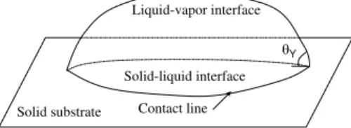
The determination of the stationary shapes of liquid drops surrounded by a vapor phase and in contact with a solid surface can be posed, since Gauss, in a variational setting consisting of obtaining the configurations of a given mass of fluid that minimize (or in general make extremal) an energy defined by
E = γlvAlv− (γsv− γsl)Asl+ EF, (1)
where γlv, γsv, and γsl denote the liquid-vapor, solid-vapor, and solid-liquid surface tensions,
respectively; Alv and Asl denote the area of the liquid-vapor and solid-liquid interfaces, respectively (see Figure 1). EF is the contribution of external forces to the total energy. If
the drop is affected by gravity, then EF =
R
Ωg · xdx, where g is the gravitational force and Ω
the domain occupied by the fluid. In absence of external forces, the configurations that minimize
c
Figure 1. Sketch of the problem.
the energy (1) are spherical caps such that the contact angle θY, called Young’s angle, between the liquid-vapor and solid-liquid interfaces satisfies
cos θY = γsvγ− γsl lv
. (2)
When the volume of fluid under consideration is sufficiently small, the contribution of gravitational forces to the energy is negligible in comparison with interfacial energies. A consistent approximation is then to ignore gravity in (1), as it is done systematically in the study of multiphase flows in microfluidic applications, for instance (see [15]). It is precisely in connection with such microfluidic applications that electric fields are incorporated with the purpose of controlling the shape and motion of small masses of fluid. This is the case, for instance, of electrowetting applications in which the shape of a mass of electrically conducting fluid is controlled via the addition of electric charges and application of external electric fields (see [10] and the references therein).
The simplest situation corresponds to a drop of perfectly conducting fluid with a total charge
Q. In this case, the energy would be given (cf. [10]) by E = γlv[Alv− (cos θY)Asl] −1
2ε0 Z
R3\Ω
|E|2dx, (3)
where E = −∇V is the electric field (V is the electric potential) created by the charges, concentrated in ∂Ω with a density σ = −ε0∂V∂n in a perfect conductor. ε0 is the dielectric
constant of the medium surrounding the drop. The potential V at the surface of a conductor is constant and, in absence of charges in R3\ Ω, is harmonic in the exterior of Ω. Hence, V is
solution of the boundary value problem
∆V = 0 at R3\ Ω, (4)
V = V0 at ∂Ω, (5)
V = O(|r|−1) as |r| → ∞. (6)
The electrical energy term in (3) can be written, after integration by parts, in the equivalent forms 1 2ε0 Z R3\Ω |E|2dx = 1 2ε0 Z ∂Ω V∂V ∂ndS = 1 2 Z ∂Ω V0σdS = 1 2QV0 = 1 2CV 2 0, (7)
where C is the capacity of Ω defined as
C = −ε0 V0 Z Ω ∂V ∂ndS. (8)
The determination of the capacity of a given set is, in general, a difficult problem. There are explicit expressions for only a few configurations, such as spheres and discs (see [8]). The best
source concerning estimation of the capacity of arbitrary sets is [12] and the related article [13]. More complex configurations, such as spherical caps, have a capacity that can be estimated from above and below but no explicit formulae. This is the main difficulty in the deduction of minimizers of (3).
By computing the first variation of the functional (3) one arrives at the following equation:
γκ − σ
2
2ε0 = −p, (9)
where γ = γlv, κ is the mean curvature (sum of the principal curvatures) of the liquid-vapor
interface at a point x, σ = −ε0∂V∂n is the surface charge density at the same point x, and p
is a constant to be determined through the constraint that the drop has a given volume. In the fluid dynamics context, p is the difference of pressure across the interface. Equation (9) has to be complemented with the boundary condition stating that the normal vector to the interface forms a constant angle with the normal to the solid substrate at any point of the contact line Γ, the set where the liquid-vapor and the solid-liquid interfaces meet. This angle has to be, exactly, θY (cf. [11]). Finally, we introduce characteristic length (Vol.)
1
3, where Vol. is
the volume of the drop, characteristic potential (Vol.)16(γε−1 0 )
1
2, characteristic surface charge
density (Vol.)−16(γε0) 1
2, and characteristic pressure γ(Vol.)− 1
3. Accordingly, we change variables
and unknowns in the form x → (Vol.)13x, V → (Vol.)16(γε−1 0 )
1
2V , σ → (Vol.)−16(γε0)12σ,
p → γ(Vol.)−13p so that space coordinates, potential, surface charge density, and pressure are
now dimensionless. We end up with the following dimensionless version of (9):
κ −σ
2
2 = −p, (10)
and the variational problem associated to the functional
E = [Alv− (cos θY)Asl] − 1 2CV
2
0, (11)
where C = −V10 RΩ∂V∂ndS, V being the solution to (4)–(6), and Ω is now a domain of unit volume.
One important motivation for this work is its relation with the phenomenon of electrowetting. This consists in the control of the wetting properties of fluids by means of electric fields. The simplest situation is that of a drop of conducting fluid connected to a battery and, therefore, kept at a given difference of potential with respect to an electrode placed at some distance below the solid substrate. In the situation studied in the present paper, such an electrode would be placed at infinity, so that we establish a given potential on the drop’s surface and assume the potential to decay at infinity. The simplest theories on electrowetting follow the original ideas of Lippmann, who developed a formula (cf. [9]) that predicts an unlimited spreading of droplets through application of sufficiently strong electrostatic potentials. Nevertheless, the physical observation is that drops do not spread infinitely but reach a saturation regime such that an increase of the potential does not produce any additional spreading but rather the appearance of instabilities at the contact line with subsequent emission of a varying number of satellite filaments (see [10] and the references therein). The demonstration of such facts, also appearing when the electrode is at a fixed distance to the drop, requires a somewhat different analysis and will be published elsewhere.
In a previous paper ([6]) we have studied, as a function θY and V0, the equilibrium
configurations. In [6] we have obtained formulae for the geometry of axially symmetric profiles in certain limits of θY and V0. We have also deduced constraints to indefinite spreading: the first one due to the fact that static solutions develop dewetted cores with the fluid concentrated in a
rim around these cores and the second constraint related to stability. By analyzing the energy functional (11) we have concluded that axially symmetric solutions must become unstable under nonaxisymmetric perturbations with n undulations (n = 2, 3, . . .), provided V0 is large enough.
In this paper we shall describe the numerical method we have used in [6] to determine for what values of V0 such instabilities do develop as a function of θY.
The paper is organized as follows. In section 2 we study the stability of the radially symmetric solutions under symmetry-breaking perturbations. In this study, we focus the theoretical discussion in the limiting cases of almost spherical and flat drops. In section 3 we explain the numerical method we have implemented in order to get results for all the intermediate cases. Finally, section 4 includes the numerical results and some conclusions.
2. Symmetry-breaking instabilities for limiting values of V0 and θY
We begin identifying values of the potential at which nonaxisymmetric solutions are energetically more favorable than the axially symmetric configurations r = a(z) (r and z are, respectively, the radial coordinate and the axis coordinate in a cylindrical coordinate system about the axis of symmetry). We perturb the profiles radially in the form
r(θ, z) = qa(z) 1 +ε22
(1 + ε cos(nθ)); z ∈ [0, H] , θ ∈ [0, 2π) . (12)
The volume of the drop does not change, since
Vol. = Z H 0 z Z 2π 0 Z ra(z) 1+ ε22 (1+ε cos(nθ)) 0 rdr dθ dz = Z H 0 z " 1 2 Z 2π 0 a2(z) 1 +ε22(1 + ε cos(nθ)) 2dθ # dz = π Z H 0 za2(z)dz.
The lateral area (area of the liquid-vapor interface) has a value (see [7])
Alv(ε) = Z H 0 Z 2π 0 q r2+ r2 θ+ r2r2zdθdz = Z H 0 Z 2π 0 rp1 + r2 z 1 + r−2r2θ p 1 + r2 z+ q 1 + r−2r2 θ+ rz2 dθdz = Z H 0 Z 2π 0 rp1 + r2 z 1 + r−2r2θ p 1 + r2 z+ q 1 + r−2r2 θ + rz2 dθdz + Z H 0 Z 2π 0 rp1 + r2 zdθdz = I1+ I2 , where I1 = Z H 0 Z 2π 0 rp1 + r2 z 1 + r−2rθ2 p 1 + r2 z+ q 1 + r−2r2 θ+ r2z dθdz ≤ Z H 0 Z 2π 0 r 2n 2ε2sin2(nθ)dθdz = n2ε2π 2 Z H 0 a(z)dz = c1n2ε2 ,
and I2= Z H 0 Z 2π 0 rp1 + r2 zdθdz = Z H 0 Z 2π 0 ap1 + a2 z · 1 −ε 2 4 + ε2 2 a2z 1 + a2 z −ε 2 4 a4z (1 + a2 z)2 + O(ε3) ¸ dθdz = Z H 0 Z 2π 0 ap1 + a2 z · 1 −ε2 4 1 (1 + a2 z)2 + O(ε3) ¸ dθdz = Alv(0) + c2ε2+ O(ε3),
while the area of the solid-liquid interface remains unchanged. Hence, we can estimate the variation of the energy under a radial perturbation:
δE = δAlv− cos θYδAsl−1
2δCV 2 0 = ε2 · (c1n2+ c2) −12 ¡ δC/ε2¢V02 ¸ + O(ε3).
Since δC/ε2 is always positive and O(1) for n > 2, as we have proved in [6], one should always
have, for
V0> V0,n=
s
2(c1n2+ c2)
(δC/ε2) , (13)
instabilities with a given n. For profiles close to a sphere V0,nis increasing with n, but this is not
the case for profiles close to a disc. Given the strict monotonicity of the capacity with n (even for profiles that are close to discs), again as we have proven in [6], and given the fact that c1 and
c2 can be made arbitrarily small for sufficiently flat profiles (when H ¿ 1), we can make the combination £(c1n2 + c2) − 12
¡
δC/ε2¢V2 0
¤
to decrease monotonically with n for configurations close to a disc. This would imply that perturbations with large n are more unstable than perturbations with a small n. Hence, one can expect the boundary to destabilize first with multiple oscillations. In the next section we implement a numerical method to compute the energy of radially perturbed equilibrium shapes and determine, for given θY, the values of the
radius of the solid-liquid interface and V0 for which instabilities with various n appear.
3. Numerical method
When dealing with radially perturbed equilibrium shapes we lose the axially symmetric properties and need to do a full three-dimensional (3D) approximation in order to compute area and capacity and hence the energy given in (11). We use a boundary element method to compute the surface charge density by solving the integral equation associated with (4), (5) and (6) in the profiles given by (12) with a unit potential at the boundary. From the surface charge density we can obtain the total charge integrating over the surface and that will be the capacity of the body.
The integral equation for the charge density at the points rp = (xp, yp, zp) of the drop’s
surface is V (rp) =4π²1 0 Z ∂Ω(t) σ(r) |r − rp|dS(r) (14)
or, since V (rp) is constant (V (rp) = 1), σ is therefore solution to
1 = 1 4π² Z ∂Ω(t) σ(r) |r − rp|dS(r). (15) 5
We approximate the boundary, ∂Ω, with a triangular mesh. The mesh is made up of N vertices and M (triangular) faces. On each face, we approximate the surface charge density with elementwise constant functions over a “virtual” element centered in each node with an area equal to 1/3 of the total area of the elements that share the node (see [16]).
We obtain the charge density from equation (15):
4πε0= C1 =
Z
∂Ω(t)
σ(r) 1
|r − ri|ds(r) i = 1, . . . , M, (16)
where ri is the barycenter of the mesh element i and M is the number of mesh elements. We approximate the integral that appears in (16) as follows:
Z ∂Ω(t) σ(r) 1 |r − ri|ds(r) ≈ M X j=1 λijσj, with λij = Z Tj 1 |r − ri|ds(r) and σj = σ(rj). (17)
Two cases are considered when calculating λij:
(i) Potential created by one element onto himself, i = j.
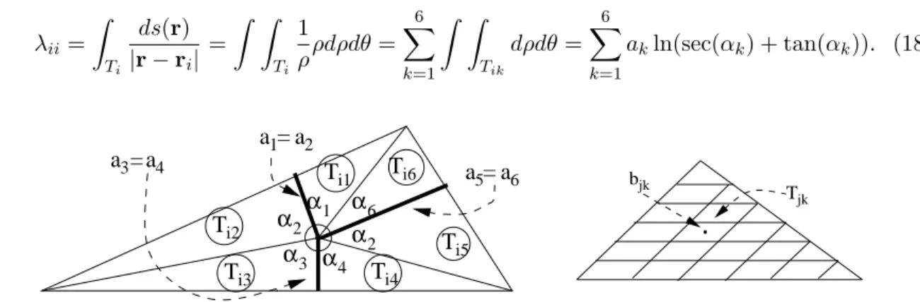
λii can be calculated exactly dividing the element Ti in six subelements as it is shown in
figure 2 (left): λii= Z Ti ds(r) |r − ri| = Z Z Ti 1 ρρdρdθ = 6 X k=1 Z Z Tik dρdθ = 6 X k=1 akln(sec(αk) + tan(αk)). (18) Ti1 Ti6 Ti2 Ti3 α2 α3 α1 Ti4 Ti5 α2 α6 α4 a1=a2 a5 a6 a4 a3 = = Tjk bjk
Figure 2. On the left: subdivision of the element Ti in six subelements for calculating the
potential created by one element onto himself. On the right: subdivision of element Tj in a variable number of subelements for calculating the potential created by element j onto element
i
(ii) Potential created by element j onto element i, i 6= j. In this case we subdivide the element
Tj in a variable number of subelements as it is shown in figure 2 (right). If we suppose that
all the charge of an element is concentrated in its center of gravity: λij =
PNs
k=1λij,k with
λij,k= ATjk
|bi−bjk|, where ATjk = area of subelement Tjk, bjk = barycenter of subelement Tjk,
bi = barycenter of element i and Ns = total number of subelements Tjk of Tj. Once all the coefficients λij are known, we calculate σ solving the system
M
X
j=1
λijσj = C1 i = 1, . . . , M, (19)
If we integrate σ over the surface of the liquid drop we will get the total charge of the drop that will coincide with the capacity of the drop because we have used V0 = 1. Once the capacity
is known we approximate numerically Alv and Asl and we get the energy of the liquid drop as a function of θy and V0 using (11).
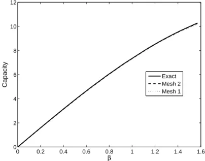
0 0.2 0.4 0.6 0.8 1 1.2 1.4 1.6 0 2 4 6 8 10 12 β Capacity Exact Mesh 2 Mesh 1
Figure 3. Capacity versus zenithal angle in an axisymmetric drop.
Figure 4. Two 3D meshes of a spherical cap (a = 0.7, β = 0.7754). On the left, mesh 1 (541 nodes and 1016 elements), and on the right, mesh 2 (2097 nodes and 4064 elements).
4. Numerical results and conclusions
Validation In order to validate the numerical method described above we have done two tests:
1. Comparison with the exact capacity of a perfectly conducting thin spherical shell. The exact capacity can be obtained through
C = 4a(sin β + β), (20)
where a is the radius of the sphere and β is the zenithal angle of the shell; see [1].
We have compared in Figure 3 the capacity obtained numerically for values of β from 0 up to π/2 (a hemispherical shell) and with two different meshes (mesh 1 and mesh 2; see Figure 4), with the exact capacity. We found with mesh 1 a maximum relative error of 0.011 and with mesh 2 a maximum relative error of 0.0058. In both cases, the relative error is below 2%.
2. Comparison with the exact capacity of a hemisphere (a spherical cap with β = π/2 and a lower tap representing the liquid-solid interface). The exact capacity of a hemisphere of radius
a is (see [8]) 4πa µ 1 −√1 3 ¶ . (21)
In this case we compare again the results obtained with meshes 1 and 2. We obtained a relative error of 0.00997 with mesh 1 and a relative error of 0.00253 with mesh 2.
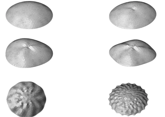
Figure 5. Shape of a radially symmetric droplet with a bottom tap of radius a = 1.16 under a potential V = 0.6 (top left). The same drop perturbed radially with n = 2 (top right), n = 3 (middle left), n = 4 (middle right), n = 10 (bottom left) and n = 20 (bottom right).
Results and discussion We have used the numerical method described above to compute the
energy of profiles perturbed in the form (12) and compare it with the energy of the axisymmetric profile a(z). We use mesh 2 for the numerical simulations. In Figure 5 we show the perturbed drops with n = 0, 2, 3, and 4 for the case corresponding to V = 0.6 and a = 1.16.
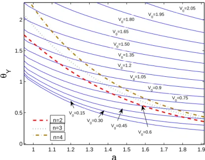
In Figure 6 we represent, together with the curves of θY as a function of a for all axisymmetric
profiles at a given potential (see [6]), the approximate “bifurcation curves” for n = 2, 3, and 4. Each of these curves, with a given value of n, delimits the regions where the configurations of the type (12) with ε ¿ 1 (that we took equal to 0.025 for our numerical computations) are energetically more favorable than configurations with smaller value of n (including the axisymmetric profiles). Notice the tendency of the curves to intersect for large values of a. This is in agreement with the discussion on profiles close to a disc in the previous section.
From Figure 6 we can obtain two important conclusions:
(i) Drops cannot be spread indefinitely by increasing the potential V0. If we trace a horizontal
line in Figure 6 for a given value of θY, we find that a increases with the potential in a
superlinear manner, but only up to some limiting value where we meet the first bifurcation curve n = 2. At this point, an axisymmetric drop is no longer the most favorable configuration, and drops with elliptic cross sections will be preferred. A further increase of
V0 leads to an intersection with the curves n = 3, 4, . . . and configurations with a higher
number of undulations would be more favorable energetically. The intersection with the first bifurcation curve takes place for relatively small values of a (in comparison with the maximum values that a may take from the constraint established in [6]. In Figure 7 we represent the axisymmetric profiles at the n = 2 bifurcation curve for different values of
θY. Observe that all the profiles are concave. Hence, the profiles changing concavity, like those represented in [6], are probably not observable in nature since nonaxisymmetric
1 1.1 1.2 1.3 1.4 1.5 1.6 1.7 1.8 1.9 0 0.5 1 1.5 2
a
θ
Y V 0=1.95 V 0=1.80 V 0=0.15 V 0=0.30 V 0=0.45 V 0=1.65 V 0=1.50 V 0=2.05 V 0=1.35 V 0=1.2 V 0=1.05 V 0=0.9 V 0=0.75 V 0=0.6 n=2 n=3 n=4Figure 6. Bifurcation branches in the a−θY plane. The bifurcations with n = 2 are represented
with dashed line, n = 3 with dotted line, and n = 4 with dash-dot line.
−20 −1.5 −1 −0.5 0 0.5 1 1.5 2
0.5
Figure 7. Axisymmetric profiles at the bifurcation curve n = 2 for θY = 1.55, 1.26, 1.03, 0.81,
0.59, 0.43.
perturbations lead to configurations which are energetically more favorable. Once a bifurcation curve has been crossed, axisymmetric drops should destabilize. This provides an explanation to the saturation effect in electrowetting.
(ii) For a given value of θY, the transition between bifurcation curves occurs relatively fast:
if we take, for instance, θY = π4, we can see that a only changes approximately from 1.4
to 1.6 while crossing the bifurcation curves n = 2, 3, and 4. This fast transition is more remarkable the smaller θY is, and for sufficiently small values of θY the transition takes place
for very flat shapes; for those shapes (see the previous section) the first bifurcation curve we cross when increasing a may correspond to n > 2. The quick transition between bifurcation curves provides an explanation of the characteristic multiple-finger patterns observed in electrowetting once saturation is reached and potential is slowly increased.
Acknowledgments
The authors thankfully acknowledge the computer resources provided by the Centro de Supercomputaci´on y Visualizaci´on de Madrid (CeSViMa) and the Spanish Supercomputing Network.
References
[1] Ashour A A 1965 On a transformation of coordinates by inversion and its application to electromagnetic induction in a thin perfectly conducting hemispherical shell Proc. London Math. Soc. 15 557–576. [2] Betel´u S I and Fontelos M A 2005 Spreading of a charged microdroplet Phys. D 209 28–35.
[3] Betel´u S I, Fontelos M A, Kindel´an U, and Vantzos O 2006 Singularities on charged viscous droplets Phys. Fluids 18 051706.
[4] Betel´u S I, Fontelos M A and Kindel´an U 2005 The shape of charged drops: Symmetry-breaking bifurcations and numerical results Elliptic and Parabolic Problems, Progr. Nonlinear Differential Equations Appl 63 51–58.
[5] Fontelos M A and Friedman A 2004 Symmetry-breaking bifurcations of charged drops Arch. Ration. Mech. Anal. 172 267–294.
[6] Fontelos M A, Kindel´an U 2008 The shape of charged drops over a solid surface and symmetry-breaking instabilities SIAM Journal of Applied Mathematics 69-1 126-148.
[7] Fontelos M A, Kindel´an U 2009 A variational approach to contact angle saturation and contact line instability in static electrowetting, QJMAM 62-4 465-480.
[8] Landkof N S 1972 Foundations of Modern Potential Theory Springer-Verlag. New York.
[9] Lippmann G 1875 Relations entre les ph´enom`enes ´electriques et capillaires Ann. Chim. Phys. 494.
[10] Mugele F and Baret J C 2005 Electrowetting: From basics to applications J. Phys. Condens. Matter 17 R705–R774.
[11] Mugele F and Buehrle J 2007 Equilibrium drop surface profiles in electric fields J. Phys. Condens. Matter 19 375112.
[12] P´olya G and Szeg¨o G 1945 Inequalities for the capacity of a condenser Amer. J. Math. 67 1–32.
[13] P´olya G and Szeg¨o G 1951 Isoperimetric Inequalities in Mathematical Physics Ann. of Math. Stud. 27, Princeton University Press, Princeton, NJ.
[14] Pozrikidis C 1992 Boundary Integral Methods for Linearized Viscous Flow Cambridge Texts Appl. Math., Cambridge University Press, UK.
[15] Stone H A, Stroock A D, and Ajdari A 2004 Engineering flows in small devices: Microfluidics toward a lab-on-a-chip, Annual Review of Fluid Mechanics 36 381–411.
[16] Zinchenko, A Z, Rother M A, Davis R H 1997, A novel boundary-integral algorithm for viscous interaction of deformable drops, Phys. Fluids 9-6.