AbstractOne of the major problem facing the data modelling at social area is multicollinearity. Multi-collinearity can have significant impact on the quality and stability of the fitted regression model. Common classical regression technique by using Least Squares estimate is highly sensitive to multicollinearity problem. In such a problem area, Partial Least Squares Regression (PLSR) is a useful and flexible tool for statistical model building; however, PLSR can only yields point estimations. This pa-per will construct the interval estimations for PLSR regression parameters by implementing Jackknife tech-nique to poverty data. A SAS macro programme is develop-ed to obtain the Jackknife interval estimator for PLSR.
KeywordsPartial Least Squares Regression, multicol- linearity, interval estimator, Jackknife
I.INTRODUCTION
ocial researchers frequently work in a situation with complex and massive amount of variables. In such situation, problem which is often faced in statistical model building is that the independent variables are many and highly collinear. This phenomenon is called multicollinearity or collinearity. Collinearity means co-dependence. This collinearity problem increases standard error of their estimated regression coefficients. The higher the collinearity among the variables, the higher of the standard error of regression coefficients. High standard error yields a wide interval estimation of para-meters. Thus, it increases risk of predictor to be rejected from regression model as non-significant variable [1].
There are a number of ways to detect multicollinearity. One of them is simply to look the correlation between variables by using scatter plot. However, this is not always good enough for a complex multicollinearity case [2]. Another approach is to compute Variance Inflation Factor (VIF). The VIF measures how much the variance of each regression coefficient is inflated because of multicollinearity compare to a situation with uncorre-lated variables. The larger the VIF, the more serious is the multicollinearity problem.
The inverse of the VIF is the tolerance. When tolerance is small, say less than 0.1, then it would indicate the present of multicollinearity. Another way to diagnose multicollinearity is through the R2 values. Multicolline-arity might exist in condition where there is a high value of R2 with a few significant coefficients or even with no significant coefficients. In a serious case of multicol-linearity, the indication can be figured out from a change
1Puji Ismartini is Student of Statistics Department Doctorate
Program, FMIPA, Institut Teknologi Sepuluh Nopember, Surabaya, 60111, Indonesia. E-mail: [email protected].
2Sony S. and Setiawan are with Department of Statistics, FMIPA,
Institut Teknologi Sepuluh Nopember, Surabaya, 60111, Indonesia. E-mail: [email protected], [email protected].
sign (positive/negative) of the regression coefficients when a new variable is added to the regression model.
In a case of multicollinearity, common classical regres-sion technique by using Least Squares yields unstable result [2]. Therefore, a such calibration technique is needed to overcome multicollinearity problem in regres-sion model.
Several methods have been developed to cope with multicollinearity problem such as Principle Component Regression (PCR), Ridge Regression (RR) and Partial Least Squares Regression (PLSR). PCR and RR are commonly used methods. However the computation process of PCR and RR is getting more complex when the number of variables is getting large. While the com-putation process of PLSR is less complex compare to those two methods. PLSR overcomes multicollinearity with smaller number of components than PCR [4]. PLSR also uses a unique way of chosing component by using singular value of decomposition of dependent and inde-pendent variables [2]. While in PCR, each component is obtained based on spectral decomposition of independent variables. So, the components in PLSR are more directly related to variability of dependent variable than PCR. It is also shown that PLSR and RR perform better than PCR [5]. Another characteristic of PLSR is statistical efficiency [6]. For moderate number of dependent va-riables, PLSR is most efficient than others [5]. Thus for some reasons, PLSR can avoid the dilemma in PCR and RR.
PLSR can only yield point estimations of their para-meters. And there is a difficulty to measure such estima-tes of accuracy for PLSR by using analytical technique. Alternatively, empirical technique such as Jackknife and Bootstrap might be used in an easy way to measure that precision [2]. Jackknife and Bootstrap are techniques for estimating standard error of an estimator through resampling process. Compare to Bootstrap, Jackknife is a useful resampling technique in a case of small sample and minimal assumption [10]. The Jackknife is also less computationally process [13] than other. The main purpose of this article is to construct the Jackknife inter-val estimation of the regression coefficient estimates in the PLSR model for poverty data analysis by developing a SAS macro program in order to measure the accuracy of PLSR coefficient regression estimators.
II.MODEL SPECIFICATION OF PARTIAL LEAST SQUARES
REGRESSION
Partial Least Squares (PLS) is method developed by Herman Wold in the 1960s as a method for constructing statistical models in a condition where the explanatory variables are many and highly collinear [3]. This method might also be used with any number of explanatory
The Jackknife Interval Estimation of
Parametersin Partial Least Squares Regression
Modelfor Poverty Data Analysis
Pudji Ismartini
1, Sony Sunaryo
2, and Setiawan
21variables which is more than the number of observation [7]. Basically, PLSR is a method which combines dimension reduction process and constructing a regres-sion model. Those two processes are performed simul-taneously in PLSR.
The general idea of PLSR is quite similar with Principle Component Regression (PCR) approach. PLSR is indirect modeling since it tries to construct a regression model by transforming a set of independent variable which is highly collinear to a set of new variable which is uncorrelated [1]. This new variables are called latent variables or components. Each component is an orthogonal linear combination of the explanatory vari-ables. Therefore, PLS has also been taken to mean “projection to latent structure”. Thus, PLS is based on latent component decompositions concept. Unlike in similar approaches such as PCR, the latent components obtained by PLSR are computed by taken into account both the independent and dependent variables of the regression [7].
To regress the response with the explanatory variables, PLSR uses Ordinary Least Squares (OLS) method. Since this estimation method does not need a strict distribution assumption. This is one of the reasons that PLSR is also addressed as a soft modeling method [8, 9].
Consider the general setting to predict q continuous response variables Y1, …, Yq using p continuous
predictor variables X1, …, Xр and the available data
sample consist of n observations. There is the nxp matrix X with vector xi = (xi1, xi2, …, xiр)Tas a row element.
Similarly, Y is the nxq matrix containing the yi = (yi1, yi2,
…, yiq)T. The latent component decomposition of PLSR
is given by
Y = TQT + F (1)
X = TPT + E (2)
Where ∈ ℝ × is a matrix of latent components,
∈ ℝ × and ∈ ℝ × are matrices of coefficients (loading matrices of response variable and predictor variables, respectively), ∈ ℝ × and ∈ ℝ × are matrices of random errors. In general, a PLSR analysis consists of the stages:
Step 1. Centering and scalling process to both response and predictor variables.
Step 2. Construct a matrix of weights (W) where
Wϵℝ .
Step 3. Construct a matrix of latent components (T) as a linear transformation of X, i.e
T = XW (3)
where the columns of W and T are wi = (wi1, wi2, …,
wрi)T and ti = (t1i, t2i, …, tni)T. Thus the equations of linear
transformation of X1, …, Xр,… are
T1 = w11X1 + … + wр1Xр
T2 = w12X1 + … + wр2Xр
… = …
Tc = w1cX1 + … + wрcXр
Step 4. Compute a matrix of component loading Q. This matrix is obtained from Equation (1) by using the least squares method.
Y = YQT
TTY = TTTQT QT = (TTT)-1 TTYQT
Step 5. Compute a matrix of regression coefficients (B) for the Y=XB+F.Since X = TWT and Y = XB
thus = TWTB. From Equation (1), Y = TQT consequently, QT = WT B. Then the solution for B can be obtained from the following equation.
WTB = QT = (TTT)-1TTY
B = WQT
= W(TTT)-1TTY (4)
Step 6. Calculate the response predictions (Ŷ)
Y = XBŶ
sinceX = TWTand
B = W(T T) T Y
Ŷ = TWTW (TTT)-1TTY
= T(TTT)-1TTY (5)
Thus, the predicted response can be calculated by only using the information of latent components and the response variable.
It is shown that the dimension reduction approach and the regression model is performed simultaneously in PLSR since it produces the matrix of regression coefficients B as well as the matrices W, T, P and Q [6].
III.THE JACKKNIFE PROCESS
Jackknife is a statistical technique which was intro-duced by Maurice Henry Quenouille in 1949 for esti-mating the bias of an estimator and to correct for it [10]. Thus, it yields a bias corrected estimator. In 1958, John Wilder Tukey proposed the variance of the estimator and hence for its standard error. It is a nonparametric method of statistical error such as the bias and standard error of an estimator [11, 12]. Since it yields standard error of an estimator, it also can compute the confidence intervals of an estimator [12]. This nonparametric technique is trustworthy since parametric analysis required assump-tions that are difficult to justifiy [11]. The advantage of the Jackknife is less computationally process [13].
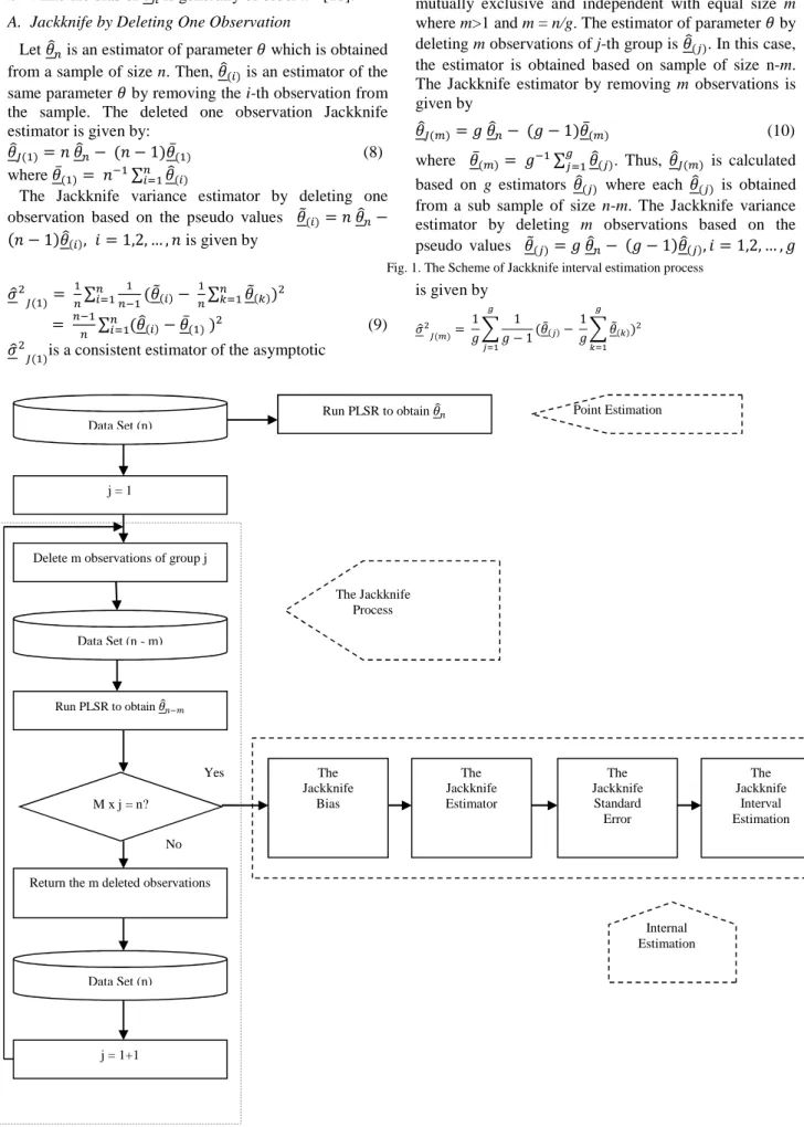
Jackknife is a versatile resampling technique. The basic idea of Jackknife is similar to cross validation procedure. In general, the process is performed by deleting one or several observations at a time and the regression coef-ficients are computed for each subset of data. This process is repeated in order to get a set of regression coefficient vectors [10, 11]. This set of coefficient vectors gives information about the variability as well as the standard error of the regression coefficients. The Jackknife is a useful resampling technique in a case of small sample and minimal assumption [10]. According to [10, 11, 14], the scheme of Jackknife process can be summarized as inFig. 1.
Let an independently and identically distributed sample of size n which is used to estimate a parameter and yields an estimator . Then, removing a group of m observations from the sample to get a set of sample of size n-m andlet be the estimator of the same para-meter based on a sample of size n-m.
The estimated bias of is reflected from the difference between and .
The Jackknife bias is calculated by using the following equation.
!"#$%&' (= () − 1)( − ) (6)
, = − !"#$%&' (
= − () − 1)( − )
If the size of deleted observation (m) is relatively small compared to n, the bias of - is generally much smaller than the bias of . The bias of - is commonly of order n-2 while the bias of is generally of order n-1 [10]. A. Jackknife by Deleting One Observation
Let is an estimator of parameter which is obtained from a sample of size n. Then, (.) is an estimator of the same parameter by removing the i-th observation from the sample. The deleted one observation Jackknife estimator is given by:
-( )= ) − () − 1) ̅( ) (8)
where ̅( )= ) ∑.1 (.)
The Jackknife variance estimator by deleting one observation based on the pseudo values 2(.)= ) −
() − 1) (.), 4 = 1,2, … , ) is given by
789
-( )= ∑.1 ( 2(.)− ∑(1 2(())9
= ∑ (.1 (.)− ̅( ) )9 (9)
789
-( )is a consistent estimator of the asymptotic
variance of and -( ).
B. Jackknife by Deleting m Observations
Suppose the sample is divided into g groups which are mutually exclusive and independent with equal size m where m>1 and m = n/g. The estimator of parameter by deleting m observations of j-th group is (&). In this case, the estimator is obtained based on sample of size n-m. The Jackknife estimator by removing m observations is given by
-( )= : − (: − 1) ̅( ) (10)
where ̅( )= : ∑;&1 (&). Thus, -( ) is calculated based on g estimators (&) where each (&) is obtained from a sub sample of size n-m. The Jackknife variance estimator by deleting m observations based on the pseudo values 2(&)= : − (: − 1) (&), 4 = 1,2, … , : is given by
789
-( )=
1 : <
1 : − 1 ;
&1
( 2(&)− 1: <2(() ;
(1 )9
Fig. 1. The Scheme of Jackknife interval estimation process
Data Set (n)
j = 1
Delete m observations of group j
Data Set (n - m)
Run PLSR to obtain
M x j = n?
Return the m deleted observations
Data Set (n)
j = 1+1
The Jackknife
Bias
The Jackknife Estimator
The Jackknife
Standard Error
The Jackknife
Interval Estimation The Jackknife
Process
Internal Estimation No
Yes
Run PLSR to obtain Point Estimation
Yes
No
= ;; ∑ (;&1 (&)− ̅( ) )9 (11) C. The Jackknife Confidence Interval
The (1-α)*100% approximate confidence intervals for parameter is given by
[ -( )− >?@( )78-( ) ; -( )+ >?@( )78-( )] (12) For large sample size, a student’s t distribution conver-ges to a standard normal distribution.
IV.APPLICATION TO POVERTY DATA
Poverty data analysis usually involves social variables which are many or highly correlated. There are many factors that might affect the poverty level in particular area. Some of those factors are demographical variables. In this case, the PLSR is applied to analyze whether number of poor people (Y) in Nanggroe Aceh Darus-salam (NAD) is influenced by number of children aged 0-4 years old (X1), number of worker (X2), number of elderly people (X3), number of school age people who are not attending school anymore (X4), and number of people who work on agriculture sector (X5). The data set is based on Socio-economic survey 2008 conducted by Statistics Indonesia (BPS).
Table 1 shows the high values of VIF for the first three predictors, since the values are over 10. There are also some tolerance values which are less than 0.1. Those indicate multicollinearity in data. The PLSR is used to analyze data by handling the multicollinearity. The result is shown below.
Table 2 illustrates the individual and cumulative variation accounted for the five PLS factors, for both the factors and the response. There are five principal components can be constructed by fivefactors. In general, Table 2 shows that the first components account for about 90 % of variation for both factors and responses. This gives a strong indication that one component are appropriate for modeling the data. It is confirmed by the cross validation analysis through the Predicted Residual Sum of Squares (PRESS) values since model with only one component yields the minimum PRESS (0.3172). Thus for this case, one component will be used in analysis. The point estimation of PLSR based on one component is given in Table 3. The accuracy of those estimations is measured from the interval estimation of the regression coefficients. And the Jackknife technique constructs the interval estimation of PLSR coefficients (Table 4).
The Jackknife confidence interval shows the interval estimations of PLSR coefficients. It also confirms that all of the factors (number of children aged 0-4 years old, number of worker, number of elderly people, number of school age people who are not attending school anymore, number of people who work on agriculture sector) are positively and significantly influence the number of poor
people in NAD. Increasing number of children aged 0-4 years old will lead to increasing number of poor people as much as 0.2054. At the same vein, the addition of a single elderly people will increase the number of poor people around 0.2129. The contribution of three other factors to the increasing number of poor is almost the same at around 0.2.
V.CONCLUSION
PLSR is a powerful method for modeling data with multicollinearity problem. PLSR yields a point estimation while its interval estimation can be constructed by using Jackknife technique. The Jackknife confidence interval also can be used to measure the accuracy of PLSR estimation. The application of PLSR and Jackknife process to poverty data analysis in NAD shows that all of the coefficients regression produced by PLSR are positively significant to measure number of poor people in that area. Thus, numbers of children aged 0-4 years old, workers, elderly people, school age people no longer attending school, and people working on agriculture sector give positive contribution to the increase of numbers of poor people in NAD.
REFERENCES
[1] D. M. Pirouz, 2006, ”An overview of partial least squares”, The
Paul Merage School of Business University of California.
[2] T. Naes, T. Isaksson, T. Fearn, and T. Davies, 2004, “Multiva-riate calibration and classification”, Chichester, UK : NIR "Publications.
[3] R. D. Tobias, 1997, “An introduction to partial least squares regression”, Cary, NC. SAS Institute.
[4] O. Yeniay, and A. Goktas, 2002, “A Comparison of partial least square regression with other prediction methods”, Hacettepe
Journal of Mathematics and Statistics, Vol.31, pp. 91-111.
[5] N. Adnan, M. H. Ahmad and R. Adnan, 2006, “A comparative study on some methods for handling multicollinearity pro-blems”, Matematika, Vol.22, No.2, pp. 109-119.
[6] A. L. Boulesteix, and K. Strimmer, 2006, “Partial least squares: a versantile tool for the analysis of high dimenstional genomic data”, Munic.
[7] A. Herve, 2007, “Partial least squares regression", Encyclopedia
of Measurement and Statistics, Thousand Oaks (CA), Sage.
[8] G. Sanchez, 2009, “Understanding partial least squares path modeling with r”, Academic Paper Universitat Politècnica de
Catalunya.
[9] N. Sellin, 1992, “Partial least squares modeling in research on educational achievement”, Otto Versand, Hamburg.
[10] R.V. Leeden, E. Meijer, and F. M. T. A. Busing, 2008, “Resampling multilevel models”, Handbook of Multilevel
Analysis, Springer.
[11] B. Efron, and G. Gong, 1983, “A leisurely look at the bootstrap, the jackknife, and cross validation”, The American Statistician, Vol. 37, No.1, pp. 36-48.
[12] F. Mosteller, and J. W. Tukey, 1977, “Data analisis and regression”, California: Addison Wesley.
[13] L. Wasserman, 2006, “All of nonparametric statistics”, Springer
Science, USA.
TABLE 1. TOLERANCE AND VIFVALUES
Model Collinearity Statistics
Tolerance VIF
X1 .045 21.987
X2 .020 50.364
X3 .082 12.262
X4 .186 5.380
X5 .205 4.871
TABLE 2.
PERCENT VARIATION AND PRESS OF PLSR
Comp. Model Effects
Dependent Variables
Root Mean PRESS Current Total Current Total
0 1.0936
1 87.8376 87.8376 92.3822 92.3822 0.3172
2 4.7803 92.6179 2.2505 94.6327 0.3424
3 4.343 96.9609 0.5184 95.1511 0.3377
4 2.5368 99.4977 0.5085 95.6596 0.3245
5 0.5023 100 0.5605 96.2201 0.348
TABLE 3.
POINT ESTIMATION OF PLSRCOEFFICIENTS
Parameter Estimates Values
β1 0.2054
β 2 0.2134
β 3 0.2129
β 4 0.1893
β 5 0.2044
TABLE 4.
ESTIMATORS OF PLSRCOEFFICIENT
Parameter
Estimates Point Estimators
Interval Estimators (95%)
Lower Bound
Upper Bound
β1 0.2054 0.18741 0.21811
Β2 0.2134 0.19146 0.23078
Β3 0.2129 0.17550 0.23738
Β4 0.1893 0.14995 0.24885
Β5 0.2044 0.19046 0.22211
Attachment
SAS Macro Program
%MACROjacknife(indata=, size=, numf=); %LET j=0;
%DO %WHILE(&j<=&size); DATA d_1;SET&indata; IF _N_=&j THEN DELETE;
ods output CenScaleParms=solution;
proc pls data=d_1 nfac=&numf method=pls details; TITLE Observation &j is deleted.;
model Y = X1 X2 X3 X4 X5 /solution; run;
proc transpose data=solution out=solution; data solution;
set solution;
rename COL1 = Beta0 COL2 = Beta1 COL3 = Beta2 COL4 = Beta3 COL5 = Beta4 COL6 = Beta5;
run;
PROC APPEND BASE = JackBeta DATA = solution force; RUN;
%LET j=%EVAL(&j+1); %END;
%MEND; data Pov11;
input WilCode $ Y X1 X2 X3 X4 X5 @@; datalines;
data value;set Jackbeta; if _N_ = 1;
proctranspose data=value out=value; data value;set value;
rename Y=OriValue; rename _NAME_=Statistik; data value;set value; label Statistik=' ';
data Jackbeta;set Jackbeta; if _N_=1 then DELETE;
procmeans data=JackBeta noprint vardef=n; var;
output out=stat(drop=_type_ _freq_); proctranspose data=stat out=stat; data stat(drop=COL2 COL3) ; set stat; rename _NAME_=Statistik;
rename COL1=n COL4=Mean COL5=STD; data stat; set stat;
label Statistik=' '; data Stat;
merge Stat value; data stat;set stat; if _N_=1 then DELETE; data stat;
set stat;
Bias = (n-1)*(Mean-OriValue); BiasCorr = OriValue-Bias; JackSTD = sqrt(n-1)* STD; t=2.074;
BatasBawah=BiasCorr-t*JackSTD; BatasAtas=BiasCorr+t*JackSTD; procprint data=Stat;
title "Hasil Simulasi Jackknife PLS"; procexport data=stat
outfile="D:\JackPov11" dbms=excel200 replace;