http://www.sciencepublishinggroup.com/j/ajdmkd doi: 10.11648/j.ajdmkd.20170204.12
Generalized Grey Target Decision Method Based on
Decision Makers’ Indifference Attribute Value Preferences
Ma Jinshan
School of Energy Science and Engineering, Henan Polytechnic University, Jiaozuo, China
Email address:
To cite this article:
Ma Jinshan.Generalized Grey Target Decision Method Based on Decision Makers’ Indifference Attribute Value Preferences. American Journal of Data Mining and Knowledge Discovery. Vol. 2, No. 4, 2017, pp. 102-108. doi: 10.11648/j.ajdmkd.20170204.12
Received: October 18, 2017; Accepted: October 31, 2017; Published: December 15, 2017
Abstract:
In multi-attribute grey target decision making, decision makers may have indifference preferences towards some attribute values such that some superior index values are no different within a small scope or some inferior index values are indifference within a small range. So the target centre domain consisting of some superior values and the target edge domain comprising some inferior values under some attribute were proposed based on the grey target decision theory. Based on the two domains, the Hamming distance of each index value to its target centre domain can be calculated. Following this, the original Hamming distances can be normalized in a linear method individually. Then the decision can be made by the integrated target centre distances considering each attribute’s weight. A case study indicated that the generalized grey target decision method improved easily and combined with other theories can address the decision makers’ indifference attribute value preferences with its concise and simple technique compared with the conventional grey target method, which is superior in handling many feasible alternatives with little difference of superior values or inferior values.Keywords:
Generalized Grey Target Decision Method, Decision Makers, Indifference Attribute Value Preferences, Target Centre Domain, Target Edge Domain1. Introduction
The grey target decision method proposed by Deng has been used in a wide range of fields [1]. Now, some scholars have made contributions to the grey target decision method. The incontinency problem of Deng’s grey transformation was tested by Chen and Xie using the simulated method [2]. Song et al. improved the calculation operators of grey target [3-5]. Zhu et al. studied the weight determination [6-8]. And the grey target decision method for mixed attributes was studied by Luo et al. [9-14]. Ma and Ji proposed a generalized grey target decision method [14, 15]. Besides, some other theories and methods were also combined with the grey target decision method [16-19]. These researches advanced the grey target decision method. However, the target centre whether expressed as a set for multiple indices or singular index discussed in above research is a point which may be determinacy for indices of real numbers or uncertainty for those of fuzzy numbers. Furthermore, the conventional target centre represents the best selection of all alternatives, which is to differentiate all indices absolutely. In practice, decision
indices to target centre indices. The generalized great target decision method can not only deal with decision makers’ indifference attribute value preferences, simplify the calculation but also be easily improved combined with other theories.
The remainder of this paper is organized as follows: Section 2 discusses the proposed method, Section 3 studies the impacts of the two domains on the index values of all alternatives under some attribute, Section 4 presents a case study, and Section 5 concludes this paper.
2. Generalized Grey Target Decision
Model
2.1. Preliminaries
Definition 1 Let S=
(
S1,S ,2 ⋯,Sn)
be an alternative set,(
1, 2, , m)
A= A A ⋯ A be an attribute set,
( 1, 2, , , 1, 2, , ) ij
S i= ⋯ n j= ⋯ m be the measure of alternative
i
S under attribute Aj, J+, J− and JM be benefit type attribute set, cost type attribute set and moderate type attribute set respectively[15], as are the bases of multi-attribute decision making.
Definition 2 Let
(
1 , 2 ,)
P P P P
m
C = C C ⋯C be a target centre index set determined by the alternative measure
( 1, 2, , , 1, 2, , ) ij
S i= ⋯ n j= ⋯ m , and Cpj satisfies
{ }
{ }
max ,
min , , 1, 2, , , 1, 2, ,
,
ij ij P
j ij ij
M j ij
S S J
C S S J i n j m
M S J
+
−
∈
= ∈ = =
∈
⋯ ⋯ (1)
where Mj is the standard or desirable value of moderate type index value, which can be given in advance [15].
Definition 3 Let
(
1 , 2 , C)
N N N N
m
C = C C ⋯ be a target edge
index set determined by the alternative measure
( 1, 2, , , 1, 2, , ) ij
S i= ⋯ n j= ⋯ m , and CNj satisfies
{ }
{ }
(
)
{
}
(
)
{
}
min ,
max ,
max , ,
max , ,
1, 2, , , 1, 2, ,
ij ij ij ij N
j M
ij ij j ij j ij
M
ij j ij ij j ij
S S J
S S J
C
S S M S M S J
S M S S M S J
i n j m
+
−
∈
∈
=
− ≥ ∈
− ≤ ∈
= ⋯ = ⋯
(2)
Definition 4 Some index values under attribute Aj reach
or better than certain value are thought as superior values without difference, as is called indifference superior attribute value preference. Similarly, some index values under attribute
j
A reach or worse than certain value are regarded as inferior values with indifference, as is called indifference inferior attribute value preference.
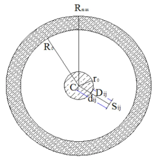
Definition 5 Given the best value CPj under attribute Aj, then the smaller scope of the value is called target centre domain. Given the worst value CNj under attribute Aj, then the smaller scope of the value is called target edge domain. The target centre domain and the target edge domain can be presented in Figure 1.
Figure 1. Target center domain and target edge domain.
In Figure 1,C0, r0, R0 and Rmax are the target centre, the radius of the target centre domain, the inner radius of the target edge domain, and the target edge respectively. The target centre and the target edge are expanded to two domains, as are shown by the shaded sections. While dijand Dij are the distances of Sijto its target centre and target centre
domain respectively.
2.2. Target Centre Domain and Target Edge Domain Determination
2.2.1. Coefficient Method
(1) Target centre domain determination
The target centre domain determined by coefficient is obtained with the best index value under attribute Aj
multiply the coefficientγ, where γ∈(0, 0.1]. Because of the small scope of target centre domain, it is better for γ no more than 0.1, which is decided by the decision makers. However, all the target centre domains determination for all attributes can employ the same coefficient or different coefficients. The following discussion limits to singular index target centre domain.
E+=[a0,b0]=[ xi0j0(1-γ),xi0j0] (3)
E-=[c0,d0]= [ xi0j0,xi0j0(1+γ)] (4)
EM=[e0,f0] =[ M0 (1-γ),M0 (1+γ)] (5)
E+ is the target centre domain of benefit type index;
a0 and b0 are the lower limits and upper limits of the target
centre domain of benefit type index respectively; E- is the target centre domain of cost type index;
c0 and d0 are the lower limits and upper limits of the target
centre domain of cost type index respectively;
EM is the target centre domain of the moderate type index;
e0 and f0 are the lower limits and upper limits of the target
centre domain of moderate type index respectively; xi0j0is the best value of all indices;
0
M is the desirable or standard value of moderate type index.
(2) Target edge domain determination
Let γN∈(0, 0.1] be the coefficient of the target edge domain, then three types of target edge domains can be determined as follows.
EN+=[aN0,bN0]= [ xNi0j0,xNi0j0(1+γN)] (6)
EN-=[cN0,dN0]= [ xNi0j0(1-γN),xNi0j0] (7)
ENM=[eN0d,fN0d] ∪[eN0u,fN0u]
=[xNm0d,xNm0d(1+γN)]∪[xNm0u(1-γN),xNm0u] (8)
where,
EN+ is the target edge domain of benefit type index;
aN0 and bN0 are the lower limits and upper limits of the target
edge domain of benefit type index respectively; EN- is the target edge domain of cost type index;
cN0 and dN0 are the lower limits and upper limits of the target
edge domain of cost type index respectively;
ENM is the target edge domain of the moderate type index;
eN0d and fN0d are the lower limits and upper limits of the
downside of the target edge domain of moderate type index respectively;
eN0u and fN0u are the lower limits and upper limits of the
upside of the target edge domain of moderate type index respectively;
xNi0j0 is the worst value of all indices;
xNm0d and xNm0u are the worst values of the downside and the
upside of the moderate value M0respectively.
2.2.2. Adjacent Value Method
(1) Target centre domain determination
The target centre domain can be determined according to the best value and the second best value under attribute Aj
with the following equations.
E+=[a0,b0]=[ xi1j1, xi0j0] (9)
E-=[c0,d0]= [ xi0j0,xi1j1] (10)
EM=[e0,f0]= [xm1d,xm1u] (11)
where,
xi1j1 is the second best value of all indices;
xm1dand xm1uare the second best values of the downside and
the upside of the moderate value M0respectively. (2) Target edge domain determination
The target edge domain can be determined by the worst value and the second worst value under attribute Aj use the
following equations.
EN+=[aN0,bN0]=[ xNi0j0, xNi1j1] (12)
EN-=[cN0,dN0]= [xNi1j1, xNi0j0] (13)
ENM=[eN0d,fN0d] ∪[eN0u,fN0u]
=[xNm0d,xNm1d]∪[xNm1u,xNm0u] (14)
where,
xNi1j1is the second worst value of all indices;
xNm1d and xNm1u are the second worst values of the downside
and the upside of the moderate value M0respectively.
2.2.3. Comprehensive Method
Coefficient method and adjacent method can be combined with each other to determine the target centre domain or the target edge domain by the decision makers’ intention. Furthermore, the two methods can also be used individually to determine the two domains. With respect to the two domains, decision makers can only determine the target centre domain or consider both of them for special purposes.
2.3. Singular Index Target Centre Distance Determination
Based on the theory of grey target decision, however the method of procedure and technique is different from the classical one is referred to as a generalized grey target method. Compared with the conventional model, the generalized grey target method has two differences: no need to normalize the index values S iij( =1, 2,⋯, ,n j=1, 2,⋯, )m and the
difference of target centre distance calculation [14, 15]. Different from the conventional grey target decision method, the proposed approach does not normalize index values beforehand.
2.3.1. Determine Target Centre Distance Considering Only Target Centre Domain
Assume x is an index value under attribute Aj, and then the distance of x to its target centre distance can be obtained.
(1) Target centre distance for benefit type index
0 0
0 0 0
0, [ , ]
, [ , ]
x a b
r
a x x a b
+
∈
=
− ∉
(15)
where E+=[a0,b0] is a target centre domain for benefit type
index, r+ is the distance of x to E+.
(2) Target centre distance for cost type index
0 0
0 0 0
0, [ , ]
, [ , ]
x c d
r
x d x c d
−
∈
=
− ∉
(16)
where E-=[c0, d0] is a target centre domain for cost type index,
r− is the distance of x to E-.
0 0
0 0
0 0
0, [ , ]
, ,
M
x e f
r e x x e
x f x f
∈
= − <
− >
(17)
where EM=[e0,f0] is a target centre domain for moderate type
index, rM is the distance of x to EM.
2.3.2. Determine Target Centre Distance Considering Target Edge Domain
The target centre distance discussed above does not consider the target edge domain. Considering both the two domains, the target centre distances of indices outside the target edge domain are still calculated by the above equations, while the target centre distances of indices in the target edge domain can be unified with the distance of the worst index value to the target centre domain. Equations (18) to (20) can be used to solve the problem.
r+max =a0-xmin (18)
where r+max is the distance of the worst index value of benefit
type to its target centre domain, xmin is the worst value.
r-max =xmax-d0 (19)
where r-max is the distance of the worst index value of cost type
to its target centre domain, xmax is the worst value.
rMmaxd=e0-xMmin orrMmaxu=xMmax-f0 (20)
where rMmaxd and rMmaxu are the downside and upside of the
distances of the worst index values of moderate type to its target centre domain respectively, xMmin and xMmax are the
worst value of the downside and the upside of the moderate value.
2.3.3. Determine Target Centre Distance Without Considering Two Domains
The target centre distance discussed above considers only the target centre domain or both the two domains. However, Equation (21) can be used to calculate the target centre distance without considering two domains.
0
r= x −x (21)
where r is the target centre distance without considering two domains, x0 and x are the target centre index and an index
value under attributeAj respectively. 2.4. Target Centre Distance Normalization
Every original singular index target centre distance can be normalized using (22).
1
, 1
ij ij n
ij i
r
z j m
r
=
= = …
∑
(22)where rij is the distance of Sijto its target centre domain under
attribute Aj, zij is the normalized target centre distance. 2.5. Weights Determination
There are three types of weight determination of attributes: objective weights, subjective weights and comprehensive weights. Since weight determination has been advanced by many scholars, this paper does not repeat it, and the interested readers can see the literature [6-8].
2.6. Decision Making
The integrated target centre distances for all alternatives can be calculated using (23).
1
, 1
m i j ij
j
w z i n
=
=
∑
ω = … (23)Thus, the decision can be made by the value wi, the smaller value of it, the better of the alternative.
2.7. Steps of the Generalized Grey Target Decision Method
Step 1 Determine every attribute’s target centre index and target edge index. Use Equations (1) and (2) to calculate the target centre indices and the target edge indices.
Step 2 Determine every attribute’s target centre domain or meanwhile determine the target edge domain. Use Equations (3) to (5) or (9) to (11) to determine the target centre domain. Use Equations (6) to (8) or (12) to (14) to determine the target edge domains.
Step 3 Calculate the Hamming distance of every index to its target centre domain use Equations (15) to (20). Without the two domains, Equation (21) can be used to calculate the target centre distance.
Step 4 Normalize every index’s target centre distance using (22).
Step 5 Determine the weights of all attributes.
Step 6 Aggregate every normalized target centre distance under all attributes using (23), then the alternative ranking can be made according to the integrated target centre distances with the smaller value the better.
3. The Impacts of Two Domains on
Alternatives
Assume S iij( =1, 2,⋯, ,n j=1, 2,⋯, )m ,S0j, and Sej are
the index value, the target centre value and the target edge value under attribute Aj respectively. Let S(i0+1)j and Si j0
be any two indices, and d(i0+1)j, d0j are their distances to
the target centre respectively. Also, let
0
(i 1)j
D + and D0j be the distances of
0
(i 1)j
S + and
0
i j
S to their target centre domain respectively. Suppose that
0
(i 1)j
d + > d0j and
0
(i 1)j
D + >D0j, the results will not change. The discussion only limits to under attribute Aj, thus the subscript j for distances will be omitted. In Figure 1, the meaning of the parameters
0
C ,r0, and Rmax are as above.
Let ∆M0 be the normalized difference of
0
(i 1)j
S + and
0
i j
S to their target centre. So Equation (22) can be obtained without considering the two domains.
0 1 0 0 1 0
0
1 1 1
i i i i
n n n
i i i
i i i
d d d d
M
d d d
+ +
= = =
−
∆ = − =
∑
∑
∑
(24)where, di is the distance of Sij to its target centre.
Suppose that there are p index values in the target centre domain, q index values in the target edge domain, while other (n-p-q) index values outside the two domains, if the two domains are both considered. Thus Equation (25) can be obtained. 0 0 0 0 1 1
1 1 1
1 1 1
1
1 1 1
i
p q n p q
i j k
i j k
i
p q n p q
i j k
i j k
i i
p q n p q
i j k
i j k
D M
D D D
D
D D D
D D
D D D
+ − − = = = − − = = = + − − = = = ∆ = + + − + + − = + +
∑
∑
∑
∑
∑
∑
∑
∑
∑
(25)Seen from Figure 1, the distance of index value to its target centre domain will be shorter than that to its original target centre, thus Equation (26) can be obtained.
0 1 0 1 0
i i
D + =d + −r ,Di0 =di0−r0 (26)
The following discussions only concern three conditions: both the two indices in the target centre domain, both of them in the target edge domain and none of them in the two domains.
(1) If S(i0+1)j and Si j0 are both included in the target centre domain, then we can achieve Equation (27) using Equation (15).
0 1 0 0
i i
D + =D = (27)
So Equation (28) can be obtained with the comparison of Equations (24) and (25).
0 1 0
M M
∆ > ∆ = (28)
Equation (28) means that the two index target distances become smaller when considering target centre domain, namely both of them are superior index values.
(2) If
0
(i 1)j
S + and
0
i j
S fall within the target edge domain, then Equation (29) can be obtained using (18).
0 1 0 0
i i
D + =D = −R r (29)
Compare with Equations (24) and (25), the following equation can be obtained:
0 1 0
M M
∆ > ∆ = (30)
Equation (30) indicates that the difference of them becomes smaller such that both of them are inferior index values considering target edge domain.
(3) If S(i0+1)j and Si j0 fall outside the two domains, then Equation (31) can be obtained by Equations (18), (26) and (25). 0 0 0 0 0 0 1 1 0
1 1 1
1
max 0 0
1 1 max 0 1 ( ) ( ) ( ) ( ) i i
p q n p q
i j k
i j k
i i
n p q k k
i i
n p q k k
d d
M
D D d r
d d
q R r d n q p r
d d
qR d n p r
+ − − = = = + − − = + − − = − ∆ = + + − − = − + − − − − = + − −
∑
∑
∑
∑
∑
(31) where, 1 0 p i i D = =∑
, max 01
( )
q j j
D q R r
=
= −
∑
, as calculated byEquations (4) and (5).
Compare with (24) and (31), their numerators are equal. So only the denominators are considered to determine the relationship of ∆M0 and ∆M1.
However the relationship of
1 n i i d =
∑
andmax 0
1
( ( ) )
n p q k k
qR d n p r
− −
=
+
∑
− − is unclear, as they aredetermined by di , Rmax , R0 , r0 , n , p and q . Therefore, the relationship of ∆M0 and ∆M1 is uncertain.
From the discussion above, we can draw the conclusion that the superior index values and inferior index values may contribute little to make a decision, and the other index values interacted with each other may act as the main roles to determine the results.
4. Case Study
4.1. Background
To evaluate coal mines’ safety performance, consider eight indices, including seam dip (°), methane emission rate (m3/t), water inflow (m3/h), spontaneous combustion period (month), ventilating structures qualified rate (%), equivalent orifice (m2), mortality per million tons (person/106t), and accident economic loss (105 Yuan) [15, 20] denoted by A1 to A10, and
the alternatives are denoted by S1 to S10. The data is shown in
Table 1, the benefit type attributes are A4 to A6, and the others
are cost type attributes. Decision makers have indifference superior value preferences towards all attributes, while have indifference inferior value preferences towards attributes A2
and A8. The target centre domain of attribute A5 is determined
by coefficient method with the value 0.05, and the others are determined by the adjacent value method. And the target edge domains of attributes A2 and A8 are determined by the adjacent
value method.
Table 1. Safety data for coal mines.
Si A1 A2 A3 A4 A5 A6 A7 A8
S1 21 6 220 12 92 1.8 0.18 381
S2 16 3.7 200 6 90 1.4 0.712 564
S3 26 9.2 180 10 88 2.7 1.34 1051.6
S4 10 4 260 8 94 1.2 0 442.5
S5 30 8.2 350 10 96 3.6 0.641 788
S6 19 5 130 12 100 2.4 0 300
S7 17 9.6 400 6 86 1.3 1.23 964.7
S8 40 14 600 6 95 2.1 1.12 885.6
S9 12 12.8 120 10 91 1.5 0.872 839.3
S10 14 5.8 155 12 89 1.7 0.426 617.2
4.2. Process to Decision Making
(1) Calculate target centre indices
The target centre indices are CP=(10, 3.7, 120, 12, 100, 3.6, 0, 300) calculated by Equation (1), and the target edge indices are CN =(40, 14, 600, 6, 86, 1.2, 1.34, 1051.6) calculated by Equation (2).
(2) Determine the target centre domain and the target edge domain
Use Equations (3), (9) and (10), target centre domains can be obtained as EP=([10, 12], [3.7, 4], [120, 130], [10, 12], [95, 100], [2.7, 3.6], [0, 0.18], [300, 381]). And use Equations (12) and (13), the target edge domains of attributes A2 and A8 are [12.8, 14] and [964.7, 1051.6]
respectively.
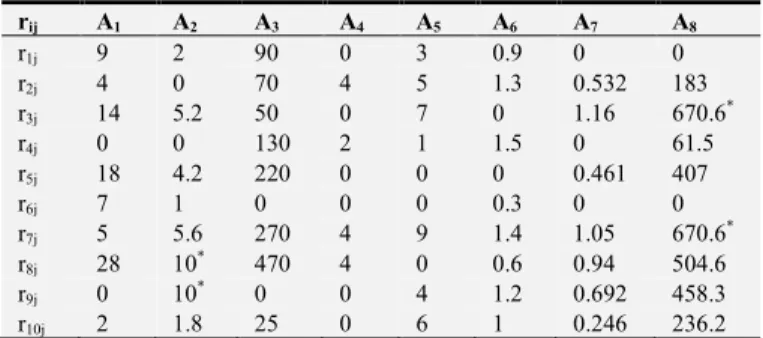
(3) Calculate original index target centre distances
Use Equations (15), 16), (18) and (19), all index target centre distances can be calculated as shown in Table 2.
Table 2. All index target centre distances.
rij A1 A2 A3 A4 A5 A6 A7 A8
r1j 9 2 90 0 3 0.9 0 0
r2j 4 0 70 4 5 1.3 0.532 183
r3j 14 5.2 50 0 7 0 1.16 670.6*
r4j 0 0 130 2 1 1.5 0 61.5
r5j 18 4.2 220 0 0 0 0.461 407
r6j 7 1 0 0 0 0.3 0 0
r7j 5 5.6 270 4 9 1.4 1.05 670.6*
r8j 28 10* 470 4 0 0.6 0.94 504.6
r9j 0 10* 0 0 4 1.2 0.692 458.3
r10j 2 1.8 25 0 6 1 0.246 236.2
Note: the value with the mark * means the value is obtained considering the target edge domain.
(4) Normalize the original target centre distances
Use Equation (22), the normalized target centre distances can be obtained shown in Table 3.
Table 3. Every index target centre distance.
Zij A1 A2 A3 A4 A5 A6 A7 A8
Z1j 0.103448 0.050251 0.067925 0 0.085714 0.109756 0 0
Z2j 0.045977 0 0.05283 0.285714 0.142857 0.158537 0.104704 0.057334
Z3j 0.16092 0.130653 0.037736 0 0.2 0 0.228302 0.210101
Z4j 0 0 0.098113 0.142857 0.028571 0.182927 0 0.019268
Z5j 0.206897 0.105528 0.166038 0 0 0 0.09073 0.127514
Z6j 0.08046 0.025126 0 0 0 0.036585 0 0
Z7j 0.057471 0.140704 0.203774 0.285714 0.257143 0.170732 0.206652 0.210101
Z8j 0.321839 0.251256 0.354717 0.285714 0 0.073171 0.185003 0.158093
Z9j 0 0.251256 0 0 0.114286 0.146341 0.136194 0.143587
Z10j 0.022989 0.045226 0.018868 0 0.171429 0.121951 0.048416 0.074002
(5) Decision making
If the attribute weights given by the experts are ω=(0.06, 0.15, 0.03, 0.08, 0.12, 0.13, 0.27, 0.16), then all the integrated target centre distances can be calculated as w=(0.040336, 0.102397, 0.149643, 0.044664, 0.078123, 0.013353, 0.195989, 0.175255, 0.130173, 0.070067)using (23). So the alternative ranking is S6≻ S1≻ S4≻ S10≻ S5≻ S2≻ S9≻
S3≻ S8≻ S7.
(6) Discussion
0.171653, 0.175819, 0.129606, 0.070067, 0.068827), So the alternative ranking is S6≻ S1≻ S4≻ S10≻ S5≻ S2≻ S9≻
S3≻ S7≻ S8.
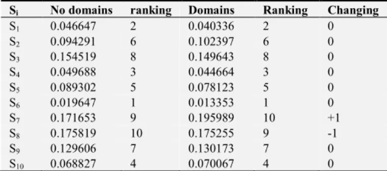
Table 4. Results comparison between the two methods.
Si No domains ranking Domains Ranking Changing
S1 0.046647 2 0.040336 2 0
S2 0.094291 6 0.102397 6 0
S3 0.154519 8 0.149643 8 0
S4 0.049688 3 0.044664 3 0
S5 0.089302 5 0.078123 5 0
S6 0.019647 1 0.013353 1 0
S7 0.171653 9 0.195989 10 +1
S8 0.175819 10 0.175255 9 -1
S9 0.129606 7 0.130173 7 0
S10 0.068827 4 0.070067 4 0
Seen from Table 4, except for the alternatives S7 and S8, the
better alternatives ranking remains steady whether considering the domains or not. Through comparing the results, we draw the conclusion that some superior index values or inferior index values contributing little to decision making. Thus, some superior index values can be thought as indifferences and the same with some inferior index values, as may not affect the decision making that seeking for some better alternatives. Meanwhile, the above results also indicate that the alternative may not be an excellent alternative with only partially better index values.
5. Conclusions
The proposed grey target decision method expanding the conventional target centre to a domain and also considering target edge domain can effectively deal with decision makers’ superior or inferior indifference attribute value preferences. The approach has its advantage to cope with multi-attribute alternatives with little difference of some index values especially for so many alternatives. It can not only simplify the calculation but also keep the accuracy of results, at least for some excellent alternatives. Moreover, decision makers can employ this method of decision making by their preferences with considering the two domains or either of them.
Acknowledgements
The authors thank the support by the Key Research Project of Science and Technology of Henan province (Grant No. 13B620033) and Doctoral Fund of Henan Polytechnic University (Grant No. B2016-53).
References
[1] Deng, J. L., Grey System Theory. 2002, Wuhan: Huazhong University of Science and Technology Press.
[2] Chen, Y. M. and H. Y. Xie, Test of the inconsistency problem on Deng’s grey transformation by simulation. Systems Engineering and Electronics, 2007. 29(8): p. 1285-1287. [3] Song, J., et al., Grey Risk Group Decision Based on the
Majorant Operator of "Rewarding Good and Punishing Bad". Journal of Grey System, 2009. 21(4): p. 377-386.
[4] Song, J., Y. G. Dang and Z. X. Wang, Multi-attribute decision model of grey target based on majorant operator of “rewarding good and punishing bad”. Systems Engineering and Electronics, 2010. 32(6).
[5] Dang, Y. G., et al., Multi-attribute decision model of grey target considering weights. Statistics and Decision, 2004(3): p. 29-30. [6] Zhu, J. J. and K. W. Hipel, Multiple stages grey target decision
making method with incomplete weight based on multi-granularity linguistic label. Information Sciences, 2012. 212: p. 15-32.
[7] Song, J., et al., The Decision-making Model of Harden Grey Target Based on Interval Number with Preference Information on Alternatives. Journal of Grey System, 2009. 21(3): p. 291-300. [8] Wang, Z. X., Y. G. Dang and H. Yang, Improvements on
decision method of grey target. Systems Engineering and Electronics, 2009. 31(11): p. 2634-2636.
[9] Luo, D. and X. Wang, The multi-attribute grey target decision method for attribute value within three-parameter interval grey number. Applied Mathematical Modelling, 2012. 36(5): p. 1957-1963.
[10] Luo, D., Multi-objective grey target decision model based on positive and negative clouts. Control and Decision, 2013. 28(2): p. 241-246.
[11] Dang, Y. G., S. F. Liu and B. Liu, Study on the Multi-attribute Decision Model of Grey Target Based on Interval Number. Engineering Science, 2005. 7(8): p. 31-35.
[12] Shen, C. G., Y. G. Dang and L. L. Pei, Hybrid multi-attribute decision model of grey target. Statistics and Decision, 2010(12): p. 17-20.
[13] Song, J., et al., New decision model of grey target with both the positive clout and negative clout. Systems engineering—
Theory & practice, 2010. 30(10): p. 1822-1827.
[14] Ma, J. S. and C. S. Ji, Generalized Grey Target Decision Method for Mixed Attributes Based on Connection Number. Journal of Applied Mathematics, 2014. 2014: p. 8.
[15] Ma, J. S., Grey Target Decision Method for a Variable Target Centre Based on the Decision Maker's Preferences. Journal of Applied Mathematics, 2014. 2014: p. 6.
[16] Wang, H. H., J. Zhu and F. Z. Geng, Grey target cluster decision method on linguistic evaluation case-based. Systems Engineering—Theory & Practice, 2013. 33(12): p. 3172-3181. [17] Zhu, J. J., et al., Grey target decision method based on
uncertain evidence aggregation under conflict interest participants. Control and Decision, 2012. 27(7): p. 1037-1046. [18] Liu, Y., et al., Multi-objective grey target decision-making based
on prospect theory. Control and Decision, 2013. 28(3): p. 345-350. [19] Zeng, B., et al., Grey target decision-making model of interval
grey number based on cobweb area. Systems Engineering and Electronics, 2013. 35(11): p. 2329-2334.