Using Analysis Tools: Goal Seek, Solver, and Data Tables

25

CHAPTER

I

n this chapter

Using Analysis Tools: Goal Seek,

Solver, and Data Tables

I

n this chapter

Analyzing Your Data with Excel 646 Using Goal Seek 646

Using Solver 650

Creating Amortization Tables to Calculate Mortgage Payments 662 Using the Analysis ToolPak Add-In 669

Analyzing Your Data with Excel

Many Excel users input data into a worksheet, use simple functions or formulas to calculate results, and then report those results to someone else. Although this is a perfectly legitimate use of Excel, it basically turns Excel into a calculator.

When you need to do more than just type data into a worksheet, you can use special Excel features to analyze your data and solve complex problems by employing variables and con-straints. Goal Seek and Solver are two great tools included with Excel that you can use to analyze data and provide answers to simple or even fairly complex problems. Goal Seek is primarily used when there is one unknown variable, and Solver when there are many vari-ables and multiple constraints. Although you might have used Solver in the past, primarily with complex tables for financial analysis, this chapter also shows you how to combine Solver with Gantt charts. Solver isn’t just for financial analysis; it can be used against pro-duction, financial, marketing, and accounting models. Solver should be used when you’re searching for a result and you have multiple variables that change (constraints). The more complex the constraints, the more you need to use Solver, as shown later in this chapter for resource loading.

Both Goal Seek and Solver enable you to play “what if” with the result of a formula when you know the result you’re shooting for, without manually changing the cells that are being referenced in the formula.

➔

Data tables in Excel provide a very important function: creating one- and two-variable tables for use in amortization and other tasks—allowing you to create a series of results based on one formula (such as cash flows). This chapter includes the details on how to set up your tables and shows a few tricks for these kinds of tables that can save you time and effort.

Whether you’re manufacturing plastic cups, hauling quantities of material or dirt, or manu-facturing digital assets in software development, Excel’s powerful analytical tools combined with structured worksheet design can make your life easier and help you manage your time more effectively.

Using Goal Seek

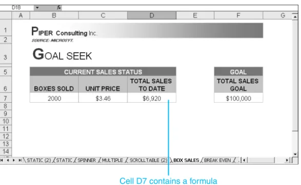
The Goal Seekfeature in Excel uses a single variable to find a desired result. To understand Goal Seek, consider this simple scenario. Suppose you’re a sales representative for a packag-ing business. You must achieve $100,000 in sales this year to receive a bonus. Figure 25.1 shows a table that displays the current situation—you have sold 2,000 units of a product with a per-unit sales price of $3.46. How many units must you sell to achieve your $100,000 goal?

Figure 25.1 Use Goal Seek to find the unknown vari-able—such as how many boxes must be sold at a unit price of $3.46 to reach $100,000 in sales.

25

N O T E

The goal amount ($100,000 in this case) must be the result of a formula, not just plain data.

Cell D7 contains a formula

At this point, you’ve probably already set up the formula in your head: (100000–6920)/3.46 = 26901.73units remaining to be sold. What would be the advantage of using a special Excel feature to calculate something so simple? Wouldn’t you just create a formula in a cell and be done with it? The advantage of Goal Seek is that you can set up your formula just once, and then substitute different amounts to get quick alternative routes to your goal. To use Goal Seek, select the formula cell (D7 in this example) and then choose Tools, Goal Seek to display the Goal Seek dialog box (see Figure 25.2). The following list describes the entries for each of the items in the dialog box:

■ Set Cell specifies the location of the formula you use to get the end result. In this case, the formula is in cell D7, and multiplies the number of units sold by the unit price. ■ Type the target value in the To Value box, which in this case is $100,000. Although you

can type the figure using commas and a dollar sign, there is no need to use those extra characters. Note that Excel does not allow you to reference a cell containing your goal. ■ In the By Changing Cell box, specify the cell location of the variable that you want to

change to reach your goal—in this case, cell B7, the cell containing the amount of boxes you need to sell to achieve your $100,000 sales goal.

As soon as you click OK or press Enter, Excel begins seeking the specified goal. In this case, the solution indicated is 28901.7341 total units at the current price of $3.46 (see Figure 25.3). You probably would need to round the solution to the nearest integer (28,902), because units aren’t generally sold in fractional amounts. To accept the proposed

Set a cell to the desired amount Have Goal Seek change the number of boxes

needed to achieve the $100,000 sales goal

changes, click OK. To return the boxes sold amount to its previous value, click Cancel. When changing the variable table you need to restore the boxes sold cell to its initial value of 2000.

25

Figure 25.2 Specify the settings in the dialog box to begin the Goal Seek process.

Figure 25.3 Goal Seek found the desired result.

Number of boxes to sell Goal to reach Set cell

Now suppose you need to determine the unit price—the other variable in the total-sales-to-date formula. If you want to sell only 2,000 units of something, how high would the price need to be for you to reach the $100,000 target? To find out, you change the By Changing Cell setting in the Goal Seek dialog box to specify cell C7, the unit price (see Figure 25.4).

Here, Goal Seek will raise the price of the boxes to a dollar value that will equal $100,000 in sales but keep the units sold at 2,000. Figure 25.5 shows the outcome: To reach $100,000 by selling only 2,000 units, each unit must cost $50. Click OK to accept the new price, or Cancel to place the old one back in.

25 Figure 25.4

In this case, Goal Seek is adjusting the unit price to reach the target.

...what unit price would you need?

Your sales goal is $100,000 If you sell 2,000 boxes...

Figure 25.5 Goal Seek is finding a unit price to meet the target.

Boxes sold is static at 2,000 Sales goal

Final unit price Goal Seek found for the unknown variable

You can use Goal Seek with complex financial models as well as with a simple solution. Link the final result cell to other cells within the model to drive the changes.

Using Solver

Goal Seek is an efficient feature for helping you reach a particular goal, but it deals with only a single variable. For most businesses, the variables are much more complex. How can you reach the profit goal if advertising expenses increase? What’s the best mix of products to increase sales in the first quarter, when revenues traditionally decline for your business? Which suppliers give you the optimal combination of price and delivery? For problems like these, you can use Solver, an add-in program that comes with Excel. This powerful analysis tool uses multiple changing variables and constraints to find the optimal solution to solve a problem. Previously, Solver was a tool used primarily for financial modeling analysis. However, Solver can be used in conjunction with models of any kind that you build in Excel. Using Solver with Gantt charts is discussed later in this section.

25

N O T E

Solver isn’t enabled by default. To add it to the Tools menu, choose Tools, Add-Ins, select Solver Add-In in the Add-Ins dialog box, and click OK. If asked to confirm, choose Yes. (You might need the Office 2003 CD, depending on how you installed the software.)

The best way to learn how to work with Solver is to experiment with simple problems, using the Solvsamp.xls file on the Office 2003 CD. When you understand how to work with multiple variables and constraints to solve a problem, you can begin using your own data and solving real business problems.

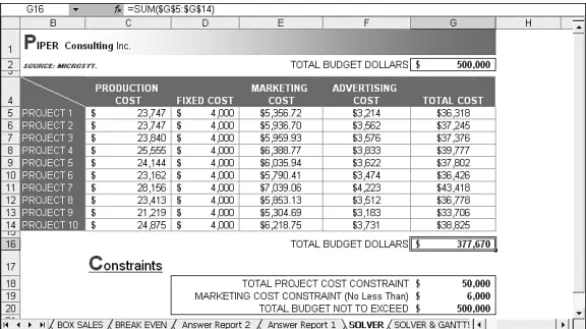
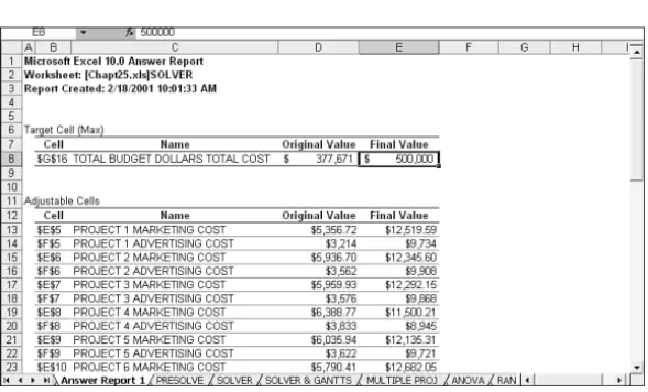
The key to understanding complex analysis tools is to start with something relatively sim-ple. The example in Figure 25.6 uses several variables to calculate a project’s total cost. What if your total budget for the year is $500,000 (as shown in the constraints cell G20) and you were using only $377,670 (as shown in cell G16)? You want each project to have a total cost of $50,000 (G5:G14) and you want to optimize or add to your marketing and advertising dollars (columns E and F). Solver will add to the Marketing cost and Advertising cost for you, adjusting your total cost for a project to $50,000.

Quite often, companies must deal with projects that have total budget caps for the year. For this, Solver works well in adjusting variables within the projects to maximize dollar amounts in certain categories, while maintaining the budget cap.

To set up this Solver scenario, follow these steps:

1. Set up the table. In the example, the production costs are in C5:C14, the fixed costs in D5:D14, the marketing costs in E5:E14, the advertising costs in F5:F14, and the totals in G5:G14.

2. Set up the constraints. In cell G18 in the example, the constraint is $50,000 for the maximum cost per project. In cell G19, the constraint is marketing costs of no less than $6,000 per project, and the total maximum budget in cell G20 is set at $500,000.

3. Select the target cell, G16, and choose Tools, Solver.

4. In the Solver Parameters dialog box, set the parameters you want to use for the prob-lem (see Figure 25.7). For this example, you want the target cell to be the total dollars spent (cell G16), which you want to equal the budget maximum, $500,000 (specified in the Value Of box). Solver will calculate the best dispersion to achieve the optimal result by adjusting the amounts in the range E5:F14 (the changing cells). ₂₅

Figure 25.6 A Solver scenario where you want all projects’ total costs to equal $50,000, while optimizing marketing and advertising costs.

Figure 25.7 Establish the target cell, the target value, and the cells that can be changed.

N O T E

For many problems, the Guess button does a great job of selecting the cells needed to effect the result. It uses the auditing feature to locate the appropriate cells.

Target cell $500,000 budget to spend

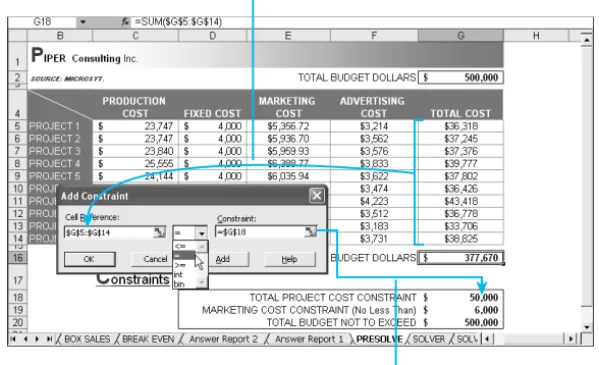
5. Next, you add constraints to the problem. Select Add to specify the first constraint. In this example, you want to spend exactly $50,000 total on each project. The constraint cell is G18, as shown in Figure 25.8.

25

Figure 25.8 Add variable con-straints you want Solver to adhere to.

The cell range for projects to include in the constraint

Can spend $50,000 per project (a constraint)

6. To add more constraints, click Add and specify the constraint. In this example, add another constraint, as shown in Figure 25.9. The marketing costs in the range E5:E14 must be greater than or equal to the constraint set in cell G19, $6,000. We still have one more constraint to enter, so click Add.

Figure 25.9 The second constraint ensures that the mar-keting dollars allo-cated to each project are greater than or equal to $6,000.

7. The last constraint is the total budget, $500,000, in cell G20 (see Figure 25.10). Don’t click Add after entering the last constraint. Instead, when the constraints are complete, click OK to go back to the Solver Parameters dialog box. Notice that all the constraints added appear in the Subject to the Constraints list (see Figure 25.11).

25 Figure 25.10

The last constraint equals $500,000, or the sum of total projects.

Figure 25.11 All the constraints appear in the Subject to the Constraints list. You can add more, change, or delete any of the constraints.

8. Click Solve or press Enter to start Solver on the problem. As Solver works, it displays a message in the status bar, as shown in Figure 25.12.

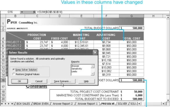
9. When Solver reaches a conclusion, it displays a dialog box that indicates the result and changes the specified values in the worksheet to reach the target. In Figure 25.13, notice the changed cells when Solver has created the optimal solution for the problem. The projects all equal $50,000 and the total budget now equals $500,000.

10. From here, you can save the Solver results and create an answer report that shows the original scenario of costs and the final result. Select Answer under Reports in the Solver Results dialog box, and click the Save Scenario button to display the dialog box shown in Figure 25.14.

Figure 25.13 Solver enables you to create reports and save scenarios so that you can later view and recall scenarios you’ve run. 25

Figure 25.12 The calculations appear in the lower left while Excel runs through all the con-straints set.

Current calculation appears in status bar

Values in these columns have changed

The total actual budget now equals $500,00

11. If you want to reset the worksheet to return to the original values, select the Restore Original Values.

Figure 25.14 Name the scenario.

25

12. Click OK and Excel will restore the values and create the answer report (see Figure 25.15). The answer report compares the original values with the changed values and indicates the cells that were changed. This way, you can compare scenarios.

C A U T I O N

Excel automatically changes the data in the constraint cells referenced by the formula (clearing the original data). If the finished scenario isn’t what you were looking for, click Restore Original Values to revert to the worksheet’s original state before trying a new scenario.

Figure 25.15 The answer report shows original values against final values, along with the cate-gory name and the adjusted cell. The tar-get cell is called out, separated at the top.

The answer report is created on a separate sheet. If you have multiple reports and sce-narios, you might want to hide the report sheet(s).

The constraints are saved with the workbook, so you don’t have to retype them each time the workbook is opened.

If Solver can’t reach a satisfactory conclusion with the data provided, a message box appears explaining Excel cannot reach a conclusion. Adjust the constraints or variables and click OK to continue attempting to solve the problem.

Solver’s solution for a complex problem might be correct but unrealistic. Be skeptical; check the appropriateness of any adjusted amounts before reporting or implementing any sugges-tion from Solver.

Solver can be very useful, but you don’t want it to run forever attempting to solve an unsolv-able problem. You can change the Solver settings before starting on the problem if you sus-pect that the solution might take a long time or require too much computing power. Clicking the Options button in the Solver Parameters dialog box displays the Solver Options dialog box, in which you can set the number of iterations of the problem that Solver will run to search for an answer or the amount of time it will spend searching before giving up. Figure 25.16 shows the options available, and Table 25.1 provides descriptions of each option.

25

N O T E

Some problems are too complex even for Solver. For problems with too many variables or constraints, try breaking the problem into segments, solving each segment separately, and then using those solutions together in Solver to reach a final conclusion.

Figure 25.16 The Solver Options dialog box enables you to set parame-ters for Solver.

Table 25.1 Solver Options Option Description

Max Time Determines the maximum amount of time Solver will search for a solution, in seconds, up to approximately nine hours.

Iterations Determines the number of times Solver will run the parameters in search of a solution.

Precision Determines the accuracy of the solution. The lower the number, the more accurate the solution.

Tolerance When integer constraints are used, it’s more difficult for Solver to solve the problem. Here, you can provide more tolerance and give up accu-racy.

Convergence For all nonlinear problems. Indicates the minimum amount of change Solver will use in each iteration. If the target cell is below the conver gence setting, Solver will offer the best solution and stop.

Assume Linear Model When checked, Solver will find a quicker solution, providing that the model is linear (using simple addition or subtraction). Nonlinear models would use growth factor and exponential smoothing or nonlinear work-sheet functions.

Assume Non-Negative Stops Solver from placing negative values in changing cells. (You also can apply constraints that indicate the value must be greater than or equal to zero.) The preceding example would use this option to prevent Solver from using negative amounts.

Use Automatic Scaling Used when the changing cells and the target cell differ by very large amounts.

Show Iteration Results Stops and enables you to view the results of each iteration in the Solver sequence.

Load Model Loads the model to use from a stored set of parameters on the work-sheet.

Save Model Saves a model to a cell or set of cells and allows you to recall the model again.

Tangent Select when the model is linear. Quadratic Select when the model is nonlinear.

Forward When cells controlled by constraints change slowly for each iteration, select this option to potentially speed up the Solver.

Central To ensure accuracy when constraint cells change rapidly and by large amounts, use this option.

Newton Uses more memory but requires fewer iterations to provide the solution. Conjugate Use with large models because it requires less memory; however, it will

use more iterations to provide a solution for the model. On complex models, if you decide to use the Conjugate set of equations, you might need to increase the Iterations box value.

Using Solver with Gantt Charts

Understanding the simple Solver scenario with constraints described in the preceding sec-tion can help you think in terms of combining Excel’s powerful tools to solve real-world problems.

25

Although I’ve worked extensively with project-management programs, I’ve found that with the proper construction of workbooks in Excel, Solver can do the following:

■ Forecast future costs

■ Track actual costs against projected costs ■ Forecast production plans

■ Track actual production against projected production ■ Forecast head count against production loads

■ Run resource-loading models for maximum efficiency

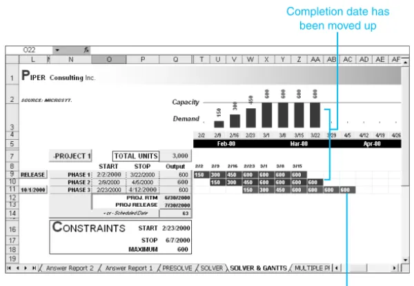
When creating timelines in Excel, you can create variations on Gantt charts (visual charts that represent information over time). You can use Gantt charts in Excel with PivotTables, Solver, and formulas to manage production plans. The key here is proper worksheet format and workbook construction. If done correctly, the workbook can be completely automated to manage the most complex productions—from managing a construction site, where quan-tities and haul times are a factor, to manufacturing digital assets in software development. Figure 25.17 shows a production model, with constraints indicated on the worksheet under the project’s Gantt chart. In this example, a project must start on a certain day (cell O9) and be completed by a certain day (P11), and there is an average number of units or quantities not to exceed per week (Q9:Q11). The target cell is the maximum number of units on the project (Q7), or any quantity you specify. Figure 25.18 shows the parameters for the first problem in the Constraints box beneath the Gantt chart setup.

25

Figure 25.17 Using Solver to opti-mize production mod-els can answer questions in seconds rather than running the scenarios m anually.

The following list describes the issues affecting the problem:

■ The original planned start date was 2/2/00, but the constraint start date is 2/23/00, indicating that the project is starting later than planned.

Figure 25.19 shows the solution. The weekly delivered average moved from 250 to 600 while still falling within the capacity of the resource. The completion date moved from 5/28 to 4/12 thus creating an earlier delivery by more than 1.5 months.

25

Start date

Completion date Average weekly output

Figure 25.18 The Solver con-straints give the pro-ject a start date, stop date (or at least com-pleted by), total quantity of units to produce, and a maxi-mum average weekly output.

■ The original stop date was 5/10/00, but the project must be completed by the con-straint set at 6/7/2000.

■ The current weekly output is 250 units per week per phase, and the constraint is set not to exceed 600.

Figure 25.19 Excel optimized the result by using the 600 “not to exceed” per week output and maximized the use of time, thus showing a schedule that com-pletes the project with almost two months to spare.

Completion date has been moved up

A Multiple-Project Solver Scenario

Based on the previous eexample and understanding how to apply constraints to production models, suppose that you have teams that have to be managed and quantities and dates you must adhere to. Solver can take multiple projects and multiple constraints and determine the optimal solution to the problem. In the example in Figure 25.20, the multiple projects over-lap, and Phase 2 of each project is the critical path in the production of the project. The total units for both projects of Phase 2 are summed at the bottom, starting in cell T22. The constraints are called out at the bottom as Start and Stop dates for each project and a maximum total output per week. On any given week, your total capacity to produce equals 600 units, but the example shows several weeks in excess of 1,000 units output in row 22. By applying the constraint to the total at the bottom, it will also take into account your capacity to produce, and find a solution. If the example isn’t possible, Excel will still find the optimal solution, given the parameters of the constraints.

25

Figure 25.20 Excel can analyze critical-path produc-tion and cycle teams, phases, or machines by applying the right constraints with the production model.

Values exceed the maximum of 600 units per week

Figure 25.21 shows the parameters used for this example. Notice how many cells are going to be changed based on the parameters or constraints supplied. All the start and stop dates have been established, as well as the maximum quantity per week not to exceed—not only per project, but also based on the overlap range starting in cell T22. This means the total capacity to output cannot exceed 600 per week for the company as a whole, so the projects’ time and output will have to be modified to fit all these variables into the Solver parameters. Not all the ranges on the Change Cells line and the Constraints box are visible. To view all the ranges, scroll down in the Subject to the Constraints list.

The settings are as follows:

■ The original start date for project 1 is set at 2/9/00 and, based on the constraints, will start on 2/23 in cell Q23. The original stop date from 4/30/00 will be constrained to 5/1/00. The maximum not to exceed per week currently is 900 and will be con-strained to 600 in cell Q27.

■ The original start date for project 2 is set at 2/23/00 and will be constrained to 4/10/00. The stop date from 6/30/00 will move to the constraint date of 7/28/00. The weekly not to exceed is constrained at no more than 600 per week in cell Q27.

■ The last constraint placed on the model will ensure that each weekly overlap unit out-put for Phase 2 (row 22) will not exceed the maximum outout-put of 600 in cell Q27. ■ The change range is from T22:BB22, which is the sum of Phase 2 of both projects

car-ried out through the length of the timeline.

Figure 25.22 shows overlap per week exceeding the weekly capacity to output in row 22. Figure 25.23 shows all the constraints placed on the project. Excel found the optimal solution.

25 Figure 25.21

You can place multi-ple constraints of start and stop dates and quantities not to exceed, and Excel will find the optimal solu-tion, taking all the variables into account.

Figure 25.22 Before Solver is used to apply constraints to the project’s start and stop dates and overall capacity to produce, the total amounts for Phase 2 of each project greatly exceed the capacity to produce.

Creating Amortization Tables to Calculate

Mortgage Payments

Excel’s Table feature helps you create structured tables for calculating mortgage and lease payments, depreciation, and so on. Suppose that you want to purchase a house; you need to see the mortgage rate based on variable percentages and mortgage amounts. Here, you would use the PMTfunction (see also Chapter 10 financial functions) to create a table to pro-vide the mortgage rate, as shown in Figure 25.24. The schedule in cells F5:F19 is calculated based on a total loan amount of $100,000 on a 30-year mortgage, with percentage rates starting at 5% and increasing in .5% increments.

25

Figure 25.23 After Solver applies the constraints to the production model, Excel provides the optimal solution, solving the problem and maintaining effi-cient project produc-tion flow.

Figure 25.24 A simple mortgage table calculates the mortgage payments based on the interest rate and the total mortgage.

The PMTfunction calculates the loan payment for a loan based on constant payments and constant interest rates.

➔

To set up a single-variable table, follow these steps:

1. In the first cell in the table, type the first interest rate percentage—for this example, you would type 5%in cell E5.

2. In the next cell down, type a formula to increase the first percentage by the increment amount. In this example, the increment is .5%, so the formula in cell E6 is =E5+0.005. This will add .5 percent to the previous percentage. Then drag the formula down to the bottom row of the table (cell E19 in this case, which will equal 12%, which is the maxi-mum interest rate you’re willing to pay).

3. In the trigger cell (cell C4 in this case), type the mortgage amount—for this example, $100,000.

4. In the target cell (cell F4 in this case), type the payment function. Here, the formula is =PMT(B4/12,360,C4)where B4/12 is the monthly interest rate, 360 is the term (30 years is 360 months), and C4 equals the total mortgage. Where cell B4 is a placeholder of zero (Excel assigns a value of zero to a blank cell referenced in a numeric formula), Excel uses the placeholder to calculate the payment needed to amortize the loan at 0%. The reason you place the mortgage in a cell rather than in the formula is that all you have to do then is change the mortgage amount. The formula references the cell and the table automatically changes, instead of your having to go into the formula and change the mortgage every time. To maximize the flexibility, you could also place the period value in a cell.

5. Select the range you want to fill. The example uses cells E4:F19. In Figure 25.25, the previous table has been deleted to rebuild the example.

25

Figure 25.25 Select the total range to build the table.

Select the entire range

Target cell Trigger cell

6. Choose Data, Table. Excel displays the Table dialog box shown in Figure 25.26. Because the interest rates in this example are listed down a column, use the Column Input Cell box to look for the interest rate used in the PMTfunction. The input cell is

always one of the arguments in the single function used for the table and corresponds to the row/column headings in the table. For example, because we have interest rates going down a column, we look for the Interestargument in the PMTfunction and use its cell reference as the column input cell.

25

Figure 25.26 The input cell is the payment needed to amortize a loan, at 0% in this case.

7. Click OK to build the table (see Figure 25.27).

Notice that by changing the mortgage amount from $100,000 to $600,000, the table automatically responds (see Figure 25.28). The advantage of using a data table is that it refers to only one formula (F4, in this example). This increases calculation speed and reduces memory use.

Figure 25.27 The final result shows the mortgage pay-ments in the body of the table, based on the corresponding percentage and mort-gage amount.

The new table is in the form of an array, which means that you can’t change the table, although you can move or delete the table. You can apply tricks to get around this limita-tion, however. You could copy the table and paste it as values using Paste Special, or you could re-create the table with a mirrored table using =. Figure 25.29 shows a mirrored table. Using a simple formula that repeats the entries in the first table (starting with cell E5), you can drag the formula to pick up all the entries in the table, which you then can manipulate. The brackets around the table formula indicates an array formula (a formula that calculates on multiple rows or ranges of data).

Figure 25.29 Create a mirrored table to get around the array formula, thus allowing you to manipulate the

formula. 25

Figure 25.28 By changing the mortgage, the table automatically responds.

Change the total value to establish mortgage payments

Creating Active Tables with Spinners

If your data tables are large, you can add special features such as form controls to make the tables easier to read and use. A spinner has been applied to the mortgage table in Figure 25.30. However, because the spinner control allows for a maximum value of 30,000, a multiplier is used in a different cell (cell C4 in this example) that multiplies the cell link in cell A1 times 50. Therefore, with every incremental change to the spinner control, it multiplies the cell link by 50.

➔

When creating the spinner, set the cell link to cell A1 in the Format Control dialog box (see Figure 25.31). Set the Maximum Value to 30,000and the Minimum Value to 0, and the Incremental Change to 1000. This means the maximum value the spinner will go up to

is 30,000, and the lowest value is 0. By adding the multiplier, you can make the mortgage table more flexible; with each click of the spin arrow, the mortgage change will be 50,000.

25

Figure 25.30 Use spinners with multipliers to drive tables.

Spinners

Figure 25.31 Set the cell link, mini-mum and maximini-mum values, as well as the incremental change as shown.

Type the multiplier formula in the table reference cell (cell C4 in this example), as shown in Figure 25.32. The formula references the cell link—the current value of the spinner—and multiplies it by 50 to give you the current principal. You hide the spinner value in cell A1 by applying a white font color.

Multiplier

Value in cell is hidden by using a white font

Multiple-Variable Tables

After learning the basic one-variable table, you can apply multiple variables to make an expanded table, referenced to different mortgage amounts (see Figure 25.33). In the previ-ous examples, you typed in the new mortgage amounts. In this instance, you reference the different cells across columns in the formula to create a broader-based table. ₂₅

Figure 25.32 Type the multiplier formula in cell C4, the table reference cell.

Figure 25.33 To create a broad-based table, the pay-ment formula references cell F4.

Adding Scrollbars to the Mortgage Table

By adding scrollbars to a table, you can span hundreds of rows and columns in a window of a few rows and columns. In the example in Figure 25.34, the interest is scrolled down to 0% and the loan amount is scrolled back to 0 in the first column (cell F6). When you scroll up, the maximum interest rate in this example is 13.7% and the maximum mortgage is $1,150,000. It normally would take multiple rows and columns of information to span

this list; however, with the proper use of scrollbars, you can create a window in which the table will scroll.

25

Figure 25.34 You can span the range of hundreds of rows and columns.

To create a scrolling window, follow these steps:

1. Create the same table setup as in the multiple-variable tables shown previously.

2. In cell E6, the beginning of the interest rate column, type the formula =A4/150, where

A4 will equal the cell link for the vertical scrollbar form control.

3. In cell F4, type the formula =$A$3*10,000, where A3 is the cell link (note the absolute

reference). Drag the formula to the right to I4.

4. Draw the scrollbar next to the interest rates, right-click it, and select Format Control (see Figure 25.35).

Figure 25.35 Draw the control and then right-click and select Format Control.

5. Format the control as follows: Current Value = 0

Minimum Value = 0 Maximum Value = 10 Incremental Change = 1 Page Change = 10 Cell Link = A4

These settings mean that the maximum value the scrollbar will reach is 10 and the low-est value is 0; each click will change the value by 1.

6. Click OK.

7. Draw the horizontal scrollbar above the house price. Right-click it and choose Format Control. Set the format control as follows:

Current Value = 0 Minimum Value = 0 Maximum Value = 100 Incremental Change = 10 Page Change = 10 Cell Link = A3

8. Click OK to finish formatting the scrollbar.

Using the Analysis ToolPak Add-In

Excel’s Analysis ToolPak(accessed by choosing Tools, Data Analysis) enables you to perform complex and sophisticated statistical analyses, with 17 statistical commands and 47 mathe-matical functions. From creating a random distribution of numbers to performing regres-sion analysis, the tools can provide the essential calculations to solve just about any problem.

25

Table 25.2 describes the various tools.

N O T E

You might need to enable the add-in before you can use it (choose Tools, Add-Ins, and select the Analysis ToolPak in the list of add-ins).

Table 25.2 Tools in the Analysis ToolPak

Tool What It Does

ANOVA: Single Factor Simple variance analysis

ANOVA: Two-Factor Variance analysis that includes more than one sample of data for each group

ANOVA: Two-Factor Variance analysis that doesn’t include more than one sample of Without Replication data for each group

Correlation Measurement—independent correlation between data sets Covariance Measurement—dependent covariance between data sets Descriptive Statistics Report of univariate statistics for sample

Exponential Smoothing Smooths data, weighting more recent data heavier F-Test: Two-Sample for Two-sample F-Test to compare population variances Variance

Histogram Counts occurrences in each of several data bins Moving Average Smooths data series by averaging the last few periods Random number generation Creates any of several types of random numbers:

Uniform—Uniform random numbers between upper and lower bounds.

Normal—Normally distributed numbers based on the mean and the standard deviation.

Bernoulli—Ones and zeros with a specified probability of success.

Poisson—A distribution of random numbers given a desired lambda.

Patterned—A sequence of numbers at a specific interval.

Discrete—Probabilities based on the predefined percents of total. Rank and Percentile Creates a report of ranking and percentile distribution

Regression Creates a table of statistics that result from least-squares regression t-Test: Paired Two-Sample Paired two-sample students t-test

for Means

t-Test: Two-Sample Paired two-sample t-test assuming equal means Assuming Equal Variances

t-Test: Two-Sample Heteroscedastic t-test Assuming Unequal Variances

z-Test: Two-Sample for Means Two-sample z-test for means with known variances Fourier Analysis DFT or FFT method, including reverse transforms Sampling Samples a population randomly or periodically

For example, suppose you want to generate random data sets to perform analysis of calls at your company’s call center based on historical data. By far, the simplest method to achieve a random sampling is using the Random Number Generation tool, which creates realistic sample data sets between ranges that you specify.

To create a random sampling, select the Random Number Generation tool in the Data Analysis dialog box. When you click OK, Excel displays the Random Number Generation dialog box, in which you can specify the parameters for the data set you want. For the exam-ple in Figure 25.37, 2 columns of variables are needed, with each column containing 15 ran-dom numbers in uniform distribution between 50 and 100. (Seven different distribution generators are available; refer to Table 25.2 for descriptions.)

25 Figure 25.36

The Data Analysis dialog box allows you to access 20 analytical tools.

Figure 25.37 Use the Random Number Generation dialog box to set para-meters for your data.

The analysis tools all work in basically the same way. Choose Tools, Data Analysis to dis-play the Data Analysis dialog box (see Figure 25.36). Select the tool you want to use, and click OK to display a separate dialog box for that particular tool.

Mortgage results Scroll dialed down

Scroll dialed down

If you don’t specify a particular number for variables or random numbers, Excel fills the cells in the Output Range.

Figure 25.38 shows the result. Figure 25.41 shows how you can use this data set for multiple analyses—just tie the analysis results to formulas, charts, and PivotTables.

25

Figure 25.38 Two sets of random numbers between 50 and 100.

Figure 25.39 Use scrollbars to cre-ate scrolling windows.

Excel in Practice

You can use tables and form controls to create automated scrolling tables. By adding scroll-bars to a table, you can span hundreds of rows and columns in a window of a few rows and columns. In the example in Figure 25.39, the interest is scrolled down to 0% and the loan amount is scrolled back to 0 in the first column (cell F6).

When you scroll up, the maximum interest rate in this example is 13.7% and the maximum mortgage is $1,150,000 as shown in Figure 25.40. It normally would take multiple rows and columns of information to span this list; however, with the proper use of scrollbars, you can create a window in which the table will scroll.

25 Figure 25.40

The scrollbar is dialed up to the maximum mortgage and interest rate.