ISSN 2307-7743 http://scienceasia.asia
KUMARASWAMY LINDLEY-POISSON DISTRIBUTION: THEORY AND APPLICATIONS
MAVIS PARARAI, BRODERICK O. OLUYEDE AND GAYAN WARAHENA-LIYANAGE
Abstract. The Kumaraswamy Lindley-Poisson (KLP) distribution which is an
ex-tension of the Lindley-Poisson Distribution [21] is introduced and its properties are explored. This new distribution represents a more flexible model for the lifetime data. Some statistical properties of the proposed distribution including the shapes of the density and hazard rate functions are explored. Moments, entropy measures and the distribution of the order statistics are given. The maximum likelihood estimation technique is used to estimate the model parameters and a simulation study is con-ducted to investigate the performance of the maximum likelihood estimates. Finally some applications of the model with real data sets are presented to illustrate the usefulness of the proposed distribution.
1. Introduction
Lindley distribution [16], studied by Lindley in the context of fiducial and Bayesian statistics, is very useful for modeling failure time data. This distribution accommodates hazard rate functions that are increasing, decreasing or constant. However, models with complex hazard rate shapes such as unimodal, bathtub and other shapes are desirable in reliability analysis, human mortality studies and related areas. Ghitany et al. [11] proposed and studied the power Lindley distribution. Properties and applications of the Lindley distribution have been studied in the context of reliability analysis by several authors including Ghitany et al. [10], Sankaran [26] and Asgharzadeh et al. [1]. Nadarajah et al. [20] proposed and developed the mathematical properties of the generalized Lindley distribution. Properties of the exponentiated Power Lindley distribution were studied by Warahena-Liyanage and Pararai [35].
Several new families of distributions have been derived by compounding the Poisson distribution with many other continuous distributions to provide more flexible distribu-tions for modeling lifetime data. Ku¸s [15] studied the exponential-Poisson distribution. Lu and Shi [17] derived and studied the Weibull-Poisson distribution. The exponen-tiated Weibull-Poisson distribution which generalizes the Weibull-Poisson was studied by Mahmoudi and Sepahdar [18], and the beta Weibull-Poisson was introduced and studied by Percontini et al.[23]. Barreto-Souza and Cribari-Neto [3] studied the ex-ponentiated exponential-Poisson distribution. The two parameter Poisson-exponential distribution with an increasing failure rate was studied by Cancho et al.[5]. Recently,
2010Mathematics Subject Classification. 60E05.
Key words and phrases. Kumaraswamy Lindley-Poisson distribution, Exponentiated Lindley Pois-son distribution, Lindley distribution, Maximum likelihood estimation.
c
2015 Science Asia
Pararai et al. [21] studied the properties of the exponentiated power Lindley-Poisson distribution, thereby generalizing the Lindley-Poisson distribution.
The properties of Kumaraswamy [14] distribution were explored in detail by Jones [13]. The author contrasted the Kumaraswamy distribution with the beta distribution. Some of the good properties of the Kumaraswamy distribution include a simple nor-malizing constant, closed form solutions of the distribution and quantile functions as well as simple formulas for the moments. Cordeiro et al. [7] studied the Kumaraswamy-Weibull distribution and applied the model to some failure data.
Motivated by the advantages of the generalized distribution with respect to having a hazard function that exhibits increasing, decreasing and bathtub shapes, as well as the versatility and flexibility of compounding Lindley and Poisson distributions in model-ing lifetime data, we propose and study a new distribution called the Kumaraswamy Lindley-Poisson (KLP) distribution, which inherits these desirable properties that also cover the shapes of quite a large number of models.
We are also motivated to study the KLP distribution because of the wide and ex-tensive usage of Lindley distribution and the fact that the current generalization still provides a useful means for its continuous extension to more complex situations. An important and positive point of the current generalization is that the Lindley distribu-tion is a basic model or exemplar of the proposed KLP distribudistribu-tion.
This paper is organized as follows. In section 2, the Kumaraswamy-G distribution (see Cordeiro and de Castro[8] for additional details), the model, its sub-models and some statistical properties including expansion of density function, quantile function, hazard function are presented. In section 3,we present the moments. Section 4 contains the distribution of the order statistics and R´enyi entropy. Mean deviations, Bonfer-onni and Lorenz curves are presented in section 5. Maximum likelihood estimates of the model parameters and asymptotic confidence intervals are given in section 6. A simulation study is also presented in section 6. Section 7 contains applications of the proposed model to real data, followed by concluding remarks in section 8.
2. The Model, Sub-models and Properties
The probability density function (pdf) and the corresponding cumulative distribution function (cdf) of the one-parameter Lindley distribution [16] are given by
(2.1) f(x;β) = β
2
β+ 1(1 +x)e
−βx, x >0, β > 0,
and
F(x) = 1−
1 + βx
β+ 1
e−βx,
(2.2)
forx >0, α, β >0, respectively.
Suppose that the random variable X has the Lindley distribution where its pdf and cdf are given in equations (2.1) and (2.2). Given N, let X1, ..., XN be independent
distributed according to the zero truncated Poisson distribution [6] with pdf
P(N =n) = θ
ne−θ
n!(1−e−θ), n= 1,2, ..., θ >0.
LetX=max(Y1, ..., YN), then the cdf of X|N =n is given by
GX|N=n(x) =
1−
1 + βx
β+ 1
e−βx
n
, x >0, β >0, θ >0,
which is the exponentiated Lindley distribution. The Lindley-Poisson (LP) distribution denoted by LP(β, θ) is defined by the marginal cdf ofX, that is,
GLP(x;β, θ) =
1−exp
θ
1−1 + β+1βx e−βx
1−eθ
(2.3)
forx >0, β >0, θ >0. The LP density function is given by
(2.4) gLP(x;β, θ) =
θβ2(1 +x)e−βxexp
θ
1−
1 + β+1βx
e−βx
(β+ 1)(eθ−1) ,
forx >0, β >0, θ >0.
2.1. Kumaraswamy Lindley Poisson Distribution. In this sub-section, we present the Kumaraswamy Lindley-Poisson (KLP) distribution and derive some of its proper-ties including the cdf, pdf, expansion of the density, hazard function, quantile function and sub-models.
Consider G(x) to be an arbitrary baseline cdf in the interval (0,1). The cdf G(x),
referred to as Kumaraswamy-G distribution [8] has cdf
F(x;a, b) = 1−(1−G(x)a)b,
where a and b are shape parameters. The pdf of the Kumaraswamy-G distribution is
given by
f(x;a, b) = abg(x)[G(x)]a−1[1−G(x)a]b−1, a >0, b >0,
(2.5)
whereg(x) = dG(x)dx is the pdf corresponding to the baseline cdf.
By takingG(x) as the cdf of the Lindley-Poisson (LP) distribution in equation (2.5), we obtain the Kumaraswamy Lindley-Poisson (KLP) distribution with a broad class of distributions that may be applicable in a wide range of day to day situations including applications in medicine, reliability and ecology. The cdf of the four-parameter KLP distribution is given by
FKLP(x) = 1− 1−
1−exp
θ
1−
1 + β+1βx
e−βx
1−eθ
forx >0, θ >0, β >0, a >0, b >0. The corresponding KLP pdf is given by
fKLP(x) =
abθβ2(1 +x)e−βxexp
θ
1−
1 + β+1βx
e−βx
(β+ 1)(eθ−1)
×
1−exp
θ
1−
1 + β+1βx
e−βx
1−eθ
a−1
×
1−
1−exp
θ
1−
1 + β+1βx
e−βx
1−eθ
a
b−1
(2.7)
forx >0, β >0, θ >0, a >0, b >0.
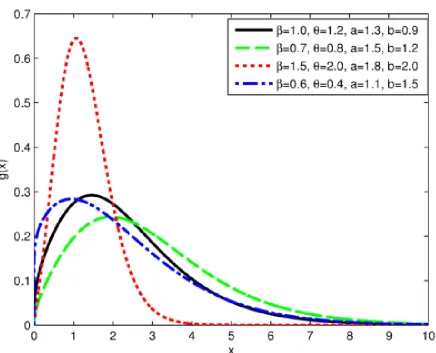
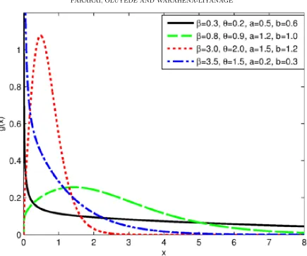
Figure 2.2. Plot of the PDF for different values of β, θ, aand b
Using the substitution λ =λ(x) = θ
1−
1 + βx
β+ 1
e−βx
, we can write the pdf
of the KLP distribution as
fKLP(x) = abθβ
2(1 +x)e−βxeλ
(β+ 1)(eθ−1)
1−eλ
1−eθ a−1
1−
1−eλ
1−eθ
ab−1 .
2.2. Expansion of the Density Function. The expansion of the pdf of KLP distri-bution is presented in this sub-section. Forb > 0 a real non-integer, we use the series representation
(1−[GLP(x)]a)b−1 =
∞
X j=0
b−1
j
(−1)j[G
LP(x)]aj,
where
GLP(x) = GLP(x;β, θ) =
exp
θ
1−
1 + βx
β+ 1
e−βx
−1
We can rewrite the density of the KLP distribution as
fKLP(x) =
∞
X j=0
(−1)j
b−1
j
abgLP(x)[GLP(x)]aj+a−1
=
abθβ2(1 +x)e−βxexp
θ
1−
1 + β+1βx
e−βx
(β+ 1)(eθ−1)
× ∞ X j=0 (−1)j
b−1
j
1−exp
θ
1−
1 + β+1βx
e−βx
1−eθ
aj+a−1
= ∞
X j,k=0
(−1)aj+a+j+k−1ab b−1 j
aj+a−1 k
[eθ(k+1)−1]
(eθ−1)(k+ 1)
×
θβ2(1 +x)e−βxexp
θ(k+ 1)
1−
1 + βx
β+ 1
e−βx
(β+ 1)[eθ(k+1)−1]
= ∞
X j,k=0
ωj,kg(x;β, θ(k+ 1)),
where
(2.8) ωj,k =ωj,k(θ, a, b) =
(−1)aj+a+j+k−1ab b−1 j
aj+a−1 k
[eθ(k+1)−1]
(eθ−1)(k+ 1)
andg(x;β, θ(k+1)) is the Lindley-Poisson pdf with parametersβ >0 andθ(k+1)>0.
This shows that the KLP distribution can be written as a linear combination of Lindley-Poisson density functions. Hence mathematical properties of the KLP distribution can be obtained from those of the LP properties.
2.3. Survival and Hazard Rate Functions. The hazard function for the KLP dis-tribution will be presented in this sub-section. Using some selected values of β, θ, a,
and b, some plots of the hazard function are presented. The hazard function of the KLP are given respectively by
hKLP(x) =
fKLP(x;β, θ, a, b)
1−FKLP(x;β, θ, a, b)
= abθβ
2(1 +x)e−βxeλ
(β+ 1)(eθ−1)
1−eλ
1−eθ a−1
1−
1−eλ
1−eθ a−1
for x > 0, β > 0, θ > 0, a > 0 and b > 0, where λ = θ
1−
1 + βx
β+ 1
e−βx
. The
suitable for monotonic and non-monotonic hazard behaviors which are more likely to be encountered in real life situations.
Figure 2.3. Plot of the Hazard Function for different values of β, θ, a
Figure 2.4. Plot of the Hazard Function for different values of β, θ, a
and b
The graph of the hazard function for different values of the parameters exhibits various shapes such as monotonically increasing and bathtub shapes.
2.4. Some sub-models of the KLP distribution. In this section, some sub-models of the KLP distribution for selected values of the parameters β, θ, a and b are presented.
• When a=b= 1, we obtain the Lindley Poisson (LP) distribution whose cdf
and pdf are given in equations (2.3) and (2.4).
• When b = 1, we obtain the exponentiated Lindley Poisson (ELP) distribution
which belongs to the resilience parameter family.
• When a=b= 1 and θ → 0+, the Lindley, (L) distribution becomes a limiting form of the KLP distribution.
• When b = 1 andθ →0+, we get the exponentiated Lindley (EL) distribution.
• When a = 1, we get the new lifetime distribution belonging to the frailty
2.5. Quantile Function. The quantile function of the KLP distribution is obtained by solving the equationF(Q(p)) = p,where 0< p <1. We therefore have
1− 1−
1−exp
θ
1−
1 + βQ(p)β+1
e−βQ(p)
1−eθ
a b =p.
UsingZ(p) =−1−β−βQ(p), we have
1− 1−
1−exp
θ 1 + Z(p) β+1
exp(Z(p) + 1 +β)
1−eθ
a b =p, so that
Z(p) exp{Z(p)}= −(β+ 1) exp(1 +β)
1− 1
θln
1−(1−eθ)(1−(1−p)1/b)1/a
,
thus,
Z(p) =W
−(β+ 1) exp(1 +β)
1− 1
θln
1−(1−eθ)(1−(1−p)1/b)1/a
.
for 0< p <1, whereW(.) is the LambertW function [9]. The quantile function of the KLP distribution is obtained by solving for Q(p) in the above equation to obtain
Q(p) = −1− 1
β −
1
βW −(
β+ 1) exp(1 +β)
1− 1
θln
1−(1−eθ)(1−(1−p)1/b)1/a
.
(2.9)
3. Moments
In this section, we present the moments of the KLP distribution. Moments are necessary and important in any statistical analysis, especially in applications. They can be used to study the most important features and characteristics of a distribution (e.g., tendency, dispersion, skewness and kurtosis).
Therth moment of a random variable X following the KLP distribution, denoted by µ0r is
µ0r = E(Xr)
= ∞
X j,k=0
ωj,kθβ2
(β+ 1)[eθ(k+1)−1] Z ∞
0
xr(1 +x)e−βx
× exp
θ(k+ 1)
1−
1 + βx
β+ 1
e−βx
dx,
(3.1)
where ωj,k is defined in equation (2.8). In order to find the moments, consider the
Lemma 1. Let
L1(β, θ(k+ 1), a, b, r) = Z ∞
0
xr(1 +x)e−βxexp
θ(k+ 1)
1−
1 + βx
β+ 1
e−βx
dx
,
then
L1(β, θ(k+ 1), a, b, r) =
∞ X m=0 m X p=0 p X q=0 q+1 X s=0 m p p q q+ 1
s
(−1)pθm(k+ 1)mβq m!(β+ 1)p
× Γ(r+s+ 1)
[β(p+ 1)]r+s+1.
Proof. Using the series expansion, ez =
∞
P p=0
zp
p!, we can rewrite the above integral as
L1(β, θ(k+ 1), a, b, r) =
∞
X m=0
θm(k+ 1)m m!
Z ∞
0
xr(1 +x)e−βx
1−
1 + βx
β+ 1
e−βx
m dx = ∞ X m=0 m X p=0 p X q=0 q+1 X s=0 m p p q q+ 1
s
(−1)pθm(k+ 1)mβq m!(β+ 1)p
×
Z ∞
0
xr+se−β(p+1)xdx.
By letting u=β(p+ 1)x, we have x= β(p+1)u and dx= β(p+1)du . Thus
Z ∞
0
xr+se−βx(p+1)dx = Γ(r+s+ 1) [β(p+ 1)]r+s+1.
By using Lemma 1, the rth moment of the KLP distribution is
µ0r = ∞ X j=0 ∞ X k=0
θβ2ωj,k
(β+ 1)[eθ(k+1)−1]L1(β, θ(k+ 1), a, b, r),
4. Order Statistics and R´enyi Entropy
4.1. Order Statistics and Entropy. Suppose that X1,· · · , Xn is a random sample
of size n from a continuous pdf, f(x). Let X1:n < X2:n < · · · < Xn:n denote the
cor-responding order statistics. IfX1,· · · , Xn is a random sample from KLP distribution,
it follows from equations (2.6) and (2.7) that the pdf of the kth order statistic, say Yk=Xk:n is given by
fk(yk) = n!fKLP(x) (k−1)!(n−k)!
n−k X j=0
n−k
j
(−1)j[FKLP(x)]j+k−1
= n!
(k−1)!(n−k)!
n−k X j=0
j+k−1 X m=0 ∞ X p,q=0 n−k
j
j+k−1
m
bm+b−1
p
×
ap+a−1
q
(−1)j+m+p+q+ap+a−1ab[eθ(q+1)−1]
(eθ−1)ap+p(q+ 1)
× θ(q+ 1)β
2(1 +x)e−βxeλ(q+1)
(β+ 1)[eθ(q+1)−1]
= ∞
X j,m,p,q=0
ϕj,m,p,q(β, θ, a, b)g(x;β, θ(q+ 1)),
where
ϕj,m,p,q(β, θ, a, b) =
n!
(k−1)!(n−k)! ∞ X j,m,p=0 ∞ X q=0 n−k
j
j+k−1
m
bm+b−1
p
×
ap+a−1
q
(−1)j+m+p+q+ap+a−1ab[eθ(q+1)−1]
(eθ−1)ap+p(q+ 1) ,
andg(x;β, θ(q+ 1)) is the LP pdf with parameters β >0 and θ(q+ 1))>0.Thus, the distribution of the kth order statistic is a linear combination of the LP distribution.
4.2. R´enyi Entropy. R´enyi entropy [24][25] is an extension of Shannon entropy [29][30].
R´enyi entropy is defined to be Hv(fKLP(x;β, θ, a, b)) = log( R∞
0 f
v
KLP(x;β,θ,a,b)dx)
1−v , where
have
Hv(fKLP) =
1 1−v
log
Z ∞
0
fKLPv (x)dx = ∞ X i,j,k=0 k X m=0 m X p=0 p+v X q=0 bv−v
i
av+ai−v j k m m p
p+v q
× (−1)
i+av+ai−v+j+m[θ(j+v)]kβp
(β+ 1)mk!(eθ−1)av+ai−v
Z ∞
0
xqe−β(v+k)xdx
= 1
1−v log ∞ X i,j,k=0 k X m=0 m X p=0 p+v X q=0 bv−v
i
av+ai−v j × k m m p
p+v q
(−1)v−av+k+p[θ(v+k]mβq
(eθ−1)j+av−v(β+ 1)pm!
×
abθβ2
(β+ 1)(eθ−1) v
Γ(q+ 1) [β(v+k)]q+1
,
forv >0, v 6= 1.
5. Mean Deviations, Bonferroni and Lorenz Curves
Deviations from the mean and median help in giving a sense of the amount of spread in a population. The mean deviation about the mean and mean deviation about the median of the KLP distribution are given by
D(µ) = 2µFKP L(µ)−2µ+
∞
X j,k=0
θβ2ω j,k
(β+ 1)[eθ(k+1)−1]L2(β, θ(k+ 1), a, b,1, µ)
and
D(M) =−µ+ ∞
X j,k=0
θβ2ω j,k
(β+ 1)[eθ(k+1)−1]L2(β, θ(k+ 1), a, b,1, M).
Consequently, Lorenz and Bonferroni curves are given by
L(FKLP(x)) =
Ry
0 tfKLP(t)dt
E(X) , and B(FKLP(x)) =
L(FKLP(x))
FKLP(x) , or
L(p) = 1
µ Z q
0
tfKLP(t)dt, and B(p) = 1
pµ Z q
0
tfKLP(t)dt,
respectively, whereq =F−1
6. Maximum Likelihood Estimation
Let x1,· · · , xn be a random sample from the KLP distribution. The log-likelihood
function is given by
L = nlog(a) +nlog(b) +nlog(θ) + 2nlog(β)−nlog(β+ 1)
+
n X
i=1
log(1 +xi)−β n X
i=0 xi+
n X
i=1
λi+ (a−1) n X
i=1
log(eλi −1)
+ (b−1)
n X
i=1
log
(eθ−1)a−(eλi −1)a
−nablog(eθ−1).
The elements of the score vector are given by
∂L ∂a = n a + n X i=1
log(eλi −1)−nblog(eθ−1)
+ (b−1)
n X
i=1
(eθ−1)alog(eθ−1)−(eλi−1)alog(eλi −1)
(eθ−1)a−(eλi −1)a ,
∂L ∂b = n b + n X i=1 log
(eθ−1)a−(eλi −1)a
−nalog(eθ−1),
∂L ∂β =
2n β −
n β+ 1 −
n X
i=1 xi +
n X
i=1 ∂λi
∂β + (a−1) n X i=1 ∂λi ∂βe λi
eλi−1
− a(b−1)
n X
i=1
eλi(eλi −1)a−1∂λi
∂β
(eθ−1)a−(eλi −1)a
and ∂L ∂θ = n θ + n X i=1
V(xi) + n X
i=1
V(xi)eλi eλi−1 −
nabeθ eθ−1
+ a(b−1)
n X
i=1
eθ(eθ−1)a−1−V(xi)eλi(eλi−1)a−1
(eθ−1)a−(eλi −1)a ,
respectively. Note that sinceλ=θ
1−
1 + βx
β+ 1
e−βx
,we have
∂λ ∂β =θe
−βx
1 + βx
β+ 1
− 1
(β+ 1)2 and ∂λ ∂θ = 1−
1 + βx
β+ 1
e−βx
=V(x).
closed form and the values of the parameters β, θ, a and b must be found by using iterative methods.
We maximize the likelihood function using NLmixed procedure in SAS as well as the function nlm in R ([32]). These functions were applied and executed for a wide range of initial values. This process often results or leads to more than one maximum, however, in these cases, we take the MLEs corresponding to the largest value of the maxima. In a few cases, no maximum was identified for the selected initial values. In these cases, a new initial value was tried in order to obtain a maximum.
The issues of existence and uniqueness of the MLEs are of theoretical interest and have been studied by several authors for different distributions including [28], [27], [34], and [33]. At this point we are not able to address the theoretical aspects (existence, uniqueness) of the MLE of the parameters of the KLP distribution.
Note that the KLP density fKLP(·;∆) has second derivatives with respect to the
parameters, so that Fisher information matrix (FIM), Iij(∆) can be expressed as
Iij(∆) =E∆
∂2log(f
KLP(X;∆)) ∂δi∂δj
, i, j = 1,2,3,4.
Elements of the FIM can be numerically obtained by MATLAB or MAPLE software. The total FIMIn(∆) can be approximated by
Jn( ˆ∆)≈
− ∂
2logL
∂δi∂δj
∆= ˆ∆
4×4
, i, j = 1,2,3,4.
(6.1)
For real data, the matrix given in equation (6.1) is obtained after the convergence of the Newton-Raphson procedure in MATLAB or R software. Let ˆ∆ = ( ˆβ,θ,ˆ ˆa,ˆb) be the maximum likelihood estimate of ∆ = (β, θ, a, b). Under the usual regularity conditions and that the parameters are in the interior of the parameter space, but not on the boundary, we have: √n( ˆ∆−∆)−→d N4(0,I−1(∆)), whereI(∆) is the expected
Fisher information matrix. The asymptotic behavior is still valid if I(∆) is replaced by the observed information matrix evaluated at ˆ∆, that is J( ˆ∆). The multivariate normal distribution with mean vector 0 = (0,0,0,0)T and covariance matrix I−1(∆) can be used to construct confidence intervals for the model parameters. That is, the approximate 100(1−η)% two-sided confidence intervals for β, θ, aand b are given by
ˆ
β±Zη/2 q
I−ββ1(∆ˆ), θˆ±Zη/2 q
I−θθ1(∆ˆ), ˆa±Zη/2 q
I−1 aa(∆ˆ),
and ˆb ± Zη/2 q
Ibb−1(∆ˆ), respectively, where I−ββ1(∆ˆ),I−θθ1(∆ˆ),I−1
aa(∆ˆ) and I
−1
bb (∆ˆ) are
diagonal elements ofI−1
n (∆ˆ) = (nI(∆ˆ))−1 andZη/2 is the upper (η/2)th percentile of a
standard normal distribution.
hypothesis if ω∗ > χ2
, where χ
2
denote the upper 100% point of the χ
2 distribution
with 2 degrees of freedom.
6.1. Monte Carlo Simulation Study. In this sub-section, we study the perfor-mance of the maximum likelihood method for estimating the KLP model parame-ters by conducting simulations for different sample sizes and different parameter val-ues. Equation in (2.9) was used to generate random data from the KLP distribu-tion. The simulation study was repeated N = 1,000 times each with samples of size
n = 100,200,400,800,1000 and parameter values I : β = 0.5, θ = 0.4, a= 0.3, b = 0.5 and II : β = 2.0, θ = 2.0, a = 0.5, b = 0.5. Four quantities were computed in this simulation study:
(a) Average bias of the MLE ˆϑ of the parameter ϑ=β, θ, a, b:
1
N N X
i=1
( ˆϑ−ϑ).
(b) Root mean squared error (RMSE) of the MLE ˆϑof the parameterϑ=β, θ, a, b:
v u u t
1
N N X
i=1
( ˆϑ−ϑ)2.
(c) Coverage probability (CP) of 95% confidence intervals of the parameter ϑ =
β, θ, a, b, i.e., the percentage of intervals that contain the true value of the parameter ϑ.
(d) Average width (AW) of 95% confidence intervals of the parameterϑ=β, θ, a, b. Table 6.1 presents the Average Bias, RMSE, CP and AW values of the parameters
β, θ, a and b for different sample sizes. According to the results, it can be concluded
that as the sample size n increases, the RMSEs decay toward zero. We also observe
Table 6.1. Monte Carlo Simulation Results: Average Bias, RMSE, CP
and AW
I II
Parameter n Average Bias RMSE CP AW Average Bias RMSE CP AW
β 100 -0.00501 0.24462 0.9510 1.51624 -0.10803 0.87209 0.9410 5.20699 200 -0.00295 0.23610 0.9490 1.13275 -0.03140 0.76234 0.9530 4.25096 400 -0.00043 0.20765 0.9480 0.91630 -0.02458 0.64276 0.9580 3.24892 800 -0.00027 0.18282 0.9450 0.70245 -0.01504 0.49704 0.9550 2.38966 1000 -0.00019 0.16592 0.9550 0.66421 -0.00511 0.45924 0.9580 2.08619
θ 100 0.88197 2.34717 0.9610 9.92480 0.84490 1.69587 0.9520 7.14813 200 0.65401 1.90481 0.9520 7.38017 0.40583 1.08716 0.9480 4.51975 400 0.61498 1.35036 0.9490 5.00112 0.18632 0.74348 0.9450 3.01703 800 0.47330 0.96665 0.9460 3.40629 0.07429 0.49949 0.9520 2.02828 1000 0.38674 0.79037 0.9510 2.87423 0.05577 0.45991 0.9490 1.80380
a 100 0.00487 0.05577 0.9480 0.29526 -0.00084 0.13179 0.9370 0.59255 200 0.00189 0.04795 0.9490 0.21880 -0.00056 0.10147 0.9420 0.43481 400 0.00046 0.03968 0.9530 0.16529 -0.00019 0.08019 0.9450 0.31945 800 0.00037 0.03462 0.9610 0.12181 -0.00013 0.05631 0.9480 0.22884 1000 0.00016 0.02995 0.9530 0.11095 -0.00103 0.05113 0.9530 0.20353
b 100 0.89313 1.65094 0.9450 10.26548 0.77219 1.75168 0.9640 10.59793 200 0.88861 1.54050 0.9490 7.79171 0.48749 1.11044 0.9540 5.20265 400 0.60264 1.13678 0.9510 4.38831 0.29611 0.72701 0.9480 2.79117 800 0.42173 0.75993 0.9420 2.50884 0.13845 0.34273 0.9560 1.21017 1000 0.31041 0.56817 0.9480 1.84970 0.12892 0.30152 0.9510 1.03431
7. Applications
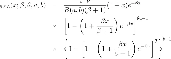
In this section, the KLP distribution is applied to real data sets in order to illus-trate the usefulness and applicability of the model. We fit the density functions of the Kumaraswamy Lindley-Poisson (KLP), Lindley-Poisson (LP) and Lindley (L) distri-butions. For comparison purposes, we also fit the beta exponentiated Lindley (BEL) distribution [22] which is also a 4 parameter model comparable to the KLP distribution. The pdf of the BEL distribution is given by
fBEL(x;β, θ, a, b) =
β2θ
B(a, b)(β+ 1)(1 +x)e −βx
×
1−
1 + βx
β+ 1
e−βx
θa−1
×
(
1−
1−
1 + βx
β+ 1
e−βx
θ)b−1
for x >0, β >0, θ >0, a >0, b > 0. Estimates of the parameters of the distributions, standard errors (in parentheses), Akaike Information Criterion (AIC = 2p−2 log( ˆL)), Consistent Akaike Information Criterion (AICC = AIC + 2p(p+1)n−p−1), Bayesian Infor-mation Criterion (BIC = plog(n)−2 log( ˆL)), where ˆL = L( ˆ∆) is the value of the likelihood function evaluated at the parameter estimates, n is the number of observa-tions, and pis the number of estimated parameters are obtained.
The first data set consists of 119 observations on fracture toughness of Alumina (Al2O3)(in the units of MPa m1/2). This data was studied by Nadarajah and Kotz
The second data set gives failure times of a sample ofn = 101 aluminum specimens of type 6061-T6 obtained by Birnbaum and Saunders [4]. These specimens were cut parallel to the direction of rolling and oscillating at 18 cycles per seconds and they were exposed to a pressure with maximum stress of 31,000 pounds per square inch (psi). The specimens were tested until failure.
The third data set that is fitted to the KLP distribution consists of breaking stress of carbon fibers which was analyzed by Bader and Priest [2]. The data represent the tensile strength, measured in GPa, of 69 carbon fibers tested under tension at gauge lengths of 20 mm.
The fourth data set set consists of 63 observations of the strengths of 1.5 cm glass fibres, originally obtained by workers at the UK National Physical Laboratory. The data was also studied by Smith and Naylor [31].
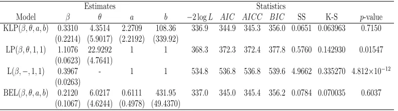
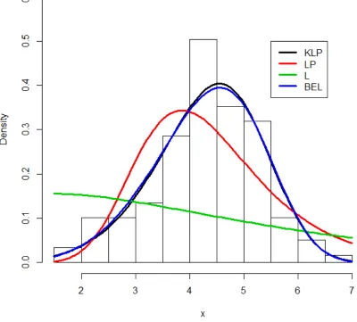
Table 7.1 displays results obtained from analyzing the Silicone Nitride data studied by Nadarajah and Kotz [19]. Estimates of the parameters of KLP distribution (s-tandard error in parentheses), Akaike Information Criterion (AIC), Consistent Akaike Information Criterion (AICC), Bayesian Information Criterion (BIC), Kolmogorov-Smirnov (K-S) statistic and its p-value are given in the Table 7.1. Plots of the fitted densities and histogram, and observed probability versus predicted probability for the Silicone Nitride data are given in Figures 7.1 and 7.2, respectively. For the probability
plot, we plottedFKLP(x(j); ˆβ,θ,ˆ a,ˆ ˆb) against j −0.375
n+ 0.25, j = 1, 2, · · · , n, wherex(j) are the ordered values of the observed data. The measures of closeness are given by the sum of squares
SS=
n X
j=1
FKLP(x(j))−
j−0.375
n+ 0.25
2 .
Table 7.1. Estimates of Models for Silicone Nitride Data
Estimates Statistics
Model β θ a b −2 logL AIC AICC BIC SS K-S p-value KLP(β, θ, a, b) 0.3310 4.3514 2.2709 108.36 336.9 344.9 345.3 356.0 0.0651 0.063963 0.7150
(0.2214) (5.9017) (2.2192) (339.92)
LP(β, θ,1,1) 1.1076 22.9292 1 1 368.3 372.3 372.4 377.8 0.5760 0.142930 0.01547 (0.0623) (4.7641)
L(β,−,1,1) 0.3967 - 1 1 534.8 536.8 536.8 539.6 4.9662 0.335270 4.812×10⁻¹²
(0.0263)
BEL(β, θ, a, b) 0.2120 6.0217 0.6111 431.95 337.0 345.0 345.4 356.2 0.0784 0.070035 0.6037 (0.1067) (4.6244) (0.4978) (49.4370)
The LR test statistics of the hypotheses H0 : LP against Ha : KLP, H0 : L against Ha : KLP, andH0 : L against Ha:LP are 27.4 (p-value=1.12×10⁻⁶ <0.001), 197.9
(p-value=1.20×10−42 <0.001) and 166.5 (p-value=4.30×10−38 <0.001).We can therefore
indicating that KLP distribution provides a better fit among the four models when fitting the Silicone Nitride data. The KLP yields the smallest value for Sum of Squares (SS) among all the models.
Table 7.2. Estimates of Models for Aluminum Specimens Data
Estimates Statistics
Model β θ a b −2 logL AIC AICC BIC SS K-S p-value KLP(β, θ, a, b) 0.0313 6.1948 3.9159 4.3329 904.4 912.4 912.8 922.8 0.0413 0.061896 0.8382
(0.0062) (23.8570) (14.5997) (2.4939)
LP(β, θ,1,1) 0.0532 96.3691 1 1 914.7 918.7 918.8 923.9 0.1759 0.100170 0.2682 (0.0033) (32.6069)
L(β,−,1,1) 0.0148 - 1 1 1106.3 1108.3 1108.3 1110.9 4.8973 0.400330 2.398×10⁻¹⁴
(0.0011)
BEL(β, θ, a, b) 0.0318 31.6377 0.6532 4.2752 904.9 912.9 912.3 923.3 0.0465 0.067242 0.7565 (0.0068) (98.0430) (2.2797) (6.0065)
Table 7.2 gives the estimates of the model parameters and the statistics AIC, AICC, BIC, K-S statistic and its p-value for the Aluminum specimen data. The LR test statistics of the hypothesesH0 : LP againstHa: KLP,H0 : L againstHa : KLP, andH0 :
L against Ha :LP are 10.3 (p-value=5.8×10⁻³ < 0.01), 201.9 (p-value=1.64×10−43 <
0.001) and 191.6 (p-value=1.42×10−43<0.001).We can therefore conclude that there
is a significant difference between KLP and LP distributions, KLP and L distributions as well as between LP and L distributions. The values of the statistics AIC, AICC and BIC are very close for the KLP and the BEL distributions. However, the KLP distribution has the smallest K-S statistic and the largest p-value indicating that KLP distribution provides a better fit among the four models when fitting the Aluminum Specimens Data. The KLP yields the smallest value for Sum of Squares (SS) among all the models. Plots of the fitted densities and histogram, observed probability versus predicted probability for the Aluminum specimen data are given in Figures 7.3 and 7.4. The plot of the fitted pdf support the conclusion based on Table 6.2. The figures suggest that both KLP and BEL distributions captures the middle part of the data, as well as the tails better than the fitted sub-models.
Table 7.3 shows the results obtained from analyzing the carbon fibers data of Bader and Priest [2].
Table 7.3. Estimates of Models for Carbon Fibers Data
Estimates Statistics
Model β θ a b −2 logL AIC AICC BIC SS K-S p-value KLP(β, θ, a, b) 0.7230 0.0348 8.3910 24.7633 97.7 105.7 106.3 114.7 0.0136 0.038759 0.9999
(6.2713) (37.1709) (33.3868) (429.21)
LP(β, θ,1,1) 2.3266 67.1553 1 1 107.8 111.8 112.0 116.3 0.1332 0.088736 0.6489 (0.1808) (24.3584)
L(β,−,1,1) 0.6545 - 1 1 238.4 240.4 240.4 242.6 3.4678 0.401130 4.547×10⁻¹⁰
(0.05803)
The LR test statistic of the hypothesis H0 : LP against Ha : KLP, H0 : L
a-gainst Ha : KLP, and H0 : L against Ha :LP are 10.1 (p-value=6.4×10⁻³, 140.7
(p-value=2.67×10⁻³⁰ <0.001) and 130.6 (p-value=3.03×10⁻³⁰ <0.001).We can therefore
conclude that there is a significant difference between KLP and LP distributions, KLP and L distributions as well as between LP and L distributions. The values of the statistics AIC, AICC and BIC are very close for the KLP and the BEL distributions. However, the KLP distribution has the smallest K-S statistic and the largest p-value indicatiing that KLP distribution provides a better fit among the four models when fitting the Carbon Fiber data. The KLP yields the smallest value for Sum of Squares (SS) among all the models.
Plots of the fitted densities and histogram, observed probability versus predicted probability for the Carbon Fiber data are given in Figures 7.5 and 7.6, respectively. The plot of the fitted pdf support the conclusion based on Table 7.4. The figures suggest that both KLP and BEL distributions capture the middle part of the data, as well as the tails better than the fitted sub-models.
Table 7.4. Estimates of Models for Glass Fibers Data
Estimates Statistics
Model β θ a b −2 logL AIC AICC BIC SS K-S p-value KLP(β, θ, a, b) 0.7334 11.8621 1.2658 2083.13 28.2 36.2 36.9 44.7 0.1529 0.13306 0.2146
(0.3463) (22.4170) (2.3915) (9883.45)
LP(β, θ,1,1) 3.0456 29.3432 1 1 59.3 63.3 63.5 67.6 0.7157 0.21887 0.004783 (0.2338) (8.3871)
L(β,−,1,1) 0.9961 - 1 1 162.6 164.6 164.6 166.7 3.3017 0.38642 1.349×10⁻⁸
(0.0948)
BEL(β, θ, a, b) 0.4705 8.0340 0.5670 8989.04 29.2 37.2 37.8 45.7 0.1951 0.14755 0.1287 (0.1995) (4.2325) (0.3193) (124.49)
Plots of the fitted densities and histogram and probability plots for the glass fibres data from Smith and Naylor [31] are given in Figures 7.7 and 7.8 respectively. The LR test statistic for the test of the hypotheses H0 : LP against Ha : KLP, H0 : L
againstHa : KLP, andH0 : L againstHa:LP are 31.1 (p-value=1.765×10−7,134.4
(p-value=6.092×10⁻²⁹ <0.0001) and 103.3 (p-value=2.88×10⁻²⁴ <0.0001), respectively.
We can therefore conclude that there is a significant difference between KLP and LP distributions, KLP and L distributions as well as between LP and L distributions.
The values of AIC, AICC and BIC shows that the KLP distribution is a better model and the SS value is comparatively smaller than the corresponding values for
the LP and L distributions. The values of these statistics (AIC, AICC, BIC) for
the KLP distribution are very competitive when compared to those of the non-nested BEL distribution. However, the KLP distribution has the smallest K-S statistic and the largest p-value indicating that KLP distribution provides a better fit among the four models when fitting the Glass Fiber data. The plot of the fitted pdf support
the conclusion based on Table 7.4. The figures suggest that both KLP and BEL
Figure 7.8. Probability Plots for Glass Fibers Data
8. Concluding Remarks
of maximum likelihood was used to estimate the model parameters. Finally, KLP dis-tribution is fitted to real data sets in order to illustrate the applicability and usefulness of the distribution.
References
[1] Asgharzedah, A., Bakouch, H. S., and Esmaeli, H., Pareto Poisson-Lindley Distribution with Applications, Journal of Applied Statistics, 40(8), (2013).
[2] Bader, M.G. and Priest, A.M.,Progress in Science and Engineering of Composites, Hayashi, T., Kawata, K. and Umekawa, S. (eds), ICCM-IV, Tokyo, pp. 1129C1136, (1982).
[3] Barreto-Souza, W., and Cribari-Neto, F.,A generalization of the exponential-Poisson distribution, Statistics and Probability Letters, 79, 2493-2500, (2009).
[4] Birnbaum, Z.W. and Saunders, S.C. A statistical model for life-length of materials, Journal of the American Statistical Association, 53, 151-160, (1958).
[5] Cancho, V.G., Louzada-Neto, F. and Barriga, G.D.C.,The Poisson-exponential lifetime distribu-tion, Computational Statistics and Data Analysis, 55, 677-686, (2011).
[6] Cohen, A. C.,Estimating Parameters in a Conditional Poisson Distribution, 16, 203-211, (1960). [7] Cordeiro, G.M., Ortega, E.M.M., and Nadarajah, S., The Kumaraswamy Weibull Distribution
with Application to Failure Data, Journal of Franklin Institute, 347, 1399-1429, (2010).
[8] Cordeiro, G.M., and de Castro, M.,A New Family of Family of Generalized Distributions, Journal of Statistical Computation and Simulations, 81(7), 883-898, (2011).
[9] Corless, R.M., Gonnet, G.H., Hare, D.E.G., Jeffrey, D.J., and D.E. Knuth, On the Lambert W function. Advances in Computational Mathematics, (5), 329-359 (1996).
[10] Ghitany, M.E., Atieh, B., and Nadarajah, S.,Lindley Distribution and Its Applications, Mathe-matics and Computers in Simulation, 78(4), 493-506 (2008).
[11] Ghitany, M.E., Al-Mutairi, D.K., Balakrishnan, N., and Al-Enezi, L.J.,Power Lindley distribu-tion and associated inference, Computational Statistics and Data Analysis, 64, 20-33 (2013). [12] Jones, M.C.,Families of distributions arising from distributions of order statistics, Test, 13, 1-43,
(2004).
[13] Jones M.C.,Kumaraswamy’s Distribution: A Beta-Type Distribution with Some Tractability Ad-vantages, Statistical Methodology, 6, 70-81, (2009).
[14] Kumaraswamy, P., A Generalized Probability Density Function for Doubly Bounded Random Process, Journal of Hydrology, 46, 79-88, (1980).
[15] Ku¸s, C¸ .,A new lifetime distribution, Computational Statistics and Data Analysis, 51, 4497-4509 (2007).
[16] Lindley, D.V.,Fiducial distributions and Bayes Theorem, Journal of the Royal Statistical Society, Series B 20,102-07, (1958).
[17] Lu, W., and Shi, D.,A New Compounding Lifetime Distribution: the Weibull-Poisson distribu-tion, Journal of Applied Statistics, 39, 21-38 (2012).
[18] Mahmoudi, E. and Sepahdar, A.,Exponentiated Weibull-Poisson distribution: Model, Properties and Applications, Mathematics and Computers in Simulation, 92, 76-97 (2013).
[19] Nadarajah, S., and Kotz, S., On the alternative to the Weibull function, Engineering Fracture Mechanics, 74, 451C456, (2007).
[20] Nadarajah, S., Bakouch, H., S., and Tahmasbi, R.,A Generalized Lindley Distribution, Sankhya B, 73, 331-359, (2011).
[21] Pararai, M., Warahena-Liyanage, G., and Oluyede, B.O.Exponentiated Power Lindley Poisson Distribution: Properties and Application, (Submitted to Communications in Statistics-Theory and Methods), (2014).
[23] Percontini, A., Blas, B. and Cordeiro, G.M, The beta Weibull Poisson distribution, Chilean Journal of Statistics, 4(2), 3-26 (2013).
[24] R´enyi, A., On Measures of Entropy and Information,Proceedings of the Fourth Berkeley Sym-posium on Mathematical Statistics and Probability, 1, 547 - 561, (1960).
[25] R´enyi, A.,On measures of entropy and information, Proceedings of the 4th Berkeley Symposium on Mathematical Statistics and Probability, vol. I, University of California Press, Berkeley, 1961, pp. 547-561.
[26] Sankaran, M.,The Discrete Poisson-Lindley DistributionBiometrics, 26, 145-149, (1970). [27] Santos Silva J. M. C., Tenreyro, S. (2010).On the Existence of Maximum Likelihood Estimates
in Poisson Regression, Economics Letters, 107, 310-312, (2010).
[28] Seregin, A. Uniqueness of the Maximum Likelihood Estimator for K-monotone Densities, Pro-ceedings of the American Mathematical Society, 138(12), 4511-4515, (2010).
[29] Shannon, E.A.,A Mathematical Theory of Communication, The Bell System Technical Journal, 27(10), 379-423, (1948).
[30] Shannon, E.A.,A Mathematical Theory of Communication, The Bell System Technical Journal, 27(10), 623-656, (1948).
[31] Smith, R. L., and Naylor, J.A comparison of maximum likelihood and Bayesian estimators for the three-parameter Weibull distribution, Applied Statistics, 36 (1987),358-369.
[32] The R Development Core Team (2011).A Language and Environment for Statistical Computing, R Foundation for Statistical Computing, (2011).
[33] Xia, J., Mi, J., Zhou, Y. Y.On the Existence and Uniqueness of the Maximum Likelihood Estima-tors of Normal and Log-normal Population Parameters with Grouped Data, Journal of Probability and Statistics., (2009).
[34] Zhou, C.Existence and Consistency of the Maximum Likelihood Estimator for the Extreme Index, J. Multivariate Analysis, 100, 794-815, (2009).
[35] Warahena-Liyanage G., Pararai M.,A Generalized Power Lindley Distribution with Applications, Asian Journal of Mathematics and Applications, 2014, Article ID ama0169, 1-23, (2014).
Mavis Pararai, Department of Mathematics, Indiana University of Pennsylvania, Indiana, PA, 15705, USA
Broderick O. Oluyede, Department of Mathematical Sciences, Georgia Southern University, Statesboro, GA, 30460, USA