Vol 6, No 6 (2015)

Available online throug

ISSN 2229 – 5046

TIME DEPENDENT PRESSURE GRADIENT EFFECT

ON UNSTEADY MHD COUETTE FLOW AND HEAT TRANSFER OF A COUPLE STRESS FLUID

V. P. RATHOD

_{AND SYEDA RASHEEDA PARVEEN*}

1

_{Department of Mathematics CNCS, Haramaya University, Ethiopia.}

2

_{Department of Studies and Research in Mathematics,}

Gulbarga University, Gulbarga-585 106, Karnataka, India.

(Received On: 20-05-15; Revised & Accepted On: 15-06-15)

ABSTRACT

T

Key –words: MHD Flow. Heat transfer, couple stress, electrically conducting fluids, unsteady pressure.

INTRODUCTION

The flow of an electrically conducting couple stress fluid under the action of a transversely applied magnetic field has applications in many devices such as magnetohydrodynamic (MHD) power generator, MHD pumps, accelerators, aerodynamics heating, electrostatic precipitation, polymer technology, petroleum industry, purification of molten metal’s from non-metallic inclusions and fluid droplets-sprays. Hartmann flow of a Newtonian fluid with heat transfer, subjected to different physical effects have been studied by many authors. [1-9].These results are important for design of the duct wall and cooling arrangements.

The flows of couple stresses fluids have many practical application in modern technology and industries, led various researchers to attempt diverse flow problems related to several Non-Newtonian fluids one such fluid that has attracted the attention of numerous researchers in fluid mechanics during the last five decades in the theory of couple stress fluid proposed by Stokes [10]. Classical theory of viscous Newtonian fluids that allow the sustenance of couple stresses and body couples in the fluid medium. The concept of couple stresses arises due to the way in which the mechanical interactions in the fluid medium are modeled. Singh and Pathak [11] have discussed unsteady flow of a dusty viscous fluid through a uniform pipe with sector of a circle as cross-section, and pulsatile flow of blood with micro-organism through a uniform pipe with sector of a circle as cross-section in the presence of transverse magnetic field has been investigated by Rathod and Parveen [12]. Also unsteady flow of a dusty magnetic conducting couple stress fluid through a pipe and the flow of a conducting fluid in a circular pipe has been investigated by many authors. Gudiraju et. al, [13], Dube and Sharma [14], Ritter and Peddison [15], Chamkha [16], investigated steady two phase vertical flow in a pipe.

Corresponding Author: Syeda Rasheeda Parveen*

2

_{Department of Studies and Research in Mathematics,}

Dube and Sharma [14] and Ritter and Peddieson [15] have reported solutions for unsteady dusty-gas flow in a circular pipe in the absence of a magnetic field and particle-phase viscous stress. Rathod and Baderunissa [17] have studied by the pulsatile flow of blood in capillaries of small exponential divergence with volume fraction of micro-organism. Rathod et. al, [18] have reported solution for couette flow of a conducting dusty visco-elastic fluid through two flat plate under the influence of transverse magnetic field. Rathod and Rasheeda [19-20] investigated unsteady flow of a dusty magnetic conducting couple stress fluid through a circular pipe and ion slip effect on the unsteady flow of a dusty couple stress fluid through a circular pipe. Rathod and Rasheeda [21] have studied by unsteady MHD couette flow with heat transfer of a couple stress fluid under exponential decaying pressure gradient. The effect of time dependent pressure gradient on unsteady dusty fluid was studied by Rukmangadachari [22] in a rectangular duct and time dependent pressure gradient effect on unsteady MHD couette flow and heat transfer of a caisson fluid was studied by Attia et. al, [23].

Attia [24] studied the influence of the Hall current on the velocity and temperature fields of an unsteady Hartmann flow of a conducting Newtonian fluid between two in finite non-conducting horizontal parallel and porous plates. Attia et. al, [23] studied time dependent pressure gradient effect on unsteady MHD couette flow and heat transfer of a caisson fluid. The extension of such problem to the case of couette flow couple stress fluid has been done in the present study. In the present work time dependent pressure gradient effect on unsteady MHD couette flow and heat transfer of a couple stress fluid. The upper plate is moving with a uniform velocity while the lower plate is stationary. The fluid is acted upon by an exponentially decaying pressure gradient, uniform suction and injection from above and below low, respectively, the fluid is also subjected to a uniform magnetic field perpendicular to the plates. The Hall current is taken into consideration while the induced magnetic field is neglected by assuming a very small magnetic Reynolds number [5]. The two plates are kept at different but constant temperature. This configuration is a good approximation of some practical situation such as heat exchangers, flow meters, and pipes that connect system components. The joule and viscous dissipations are taken into consideration in the energy equation. The governing momentum and energy equation are solved by using transform technique. [cosine transform (25)]. The inclusion of magnetic field, unsteady pressure gradient, the Hall current, the suction and injection, and also couple stress parameter leads to some interesting effects on both the velocity and temperature fields.

FORMULATION OF THE PROBLEM

The fluid is assumed to be laminar, incompressible and obeying a flows between Two infinite horizontal plates located at the y = ±h planes and extend from x = - ∞ to ∞ and from z = ∞ to ∞. The upper plate is suddenly set into motion and moves with a uniform velocity 𝑢𝑢₀, while the lower plate is stationary. The upper plate is simultaneously subjected to a step change in temperature from T1toT2. then, the upper and lower plates are kept at two constant temperatures

T2&T1 respectively, with T2>T1 the fluid is acted upon by an exponentially decaying pressure gradient 𝜕𝜕𝜕𝜕_{𝜕𝜕𝜕𝜕} in the

x-direction, and a uniform suction from above and injection from below which are applied at t = o, a uniform magnetic field 𝐵𝐵₀ is applied in the positive y–direction and is assumed undisturbed as the induced magnetic field is neglected by assuming a very small magnetic Reynolds number [4]. The Hall effect is taken into consideration and consequently a z – component for the velocity is expected to arise. The uniform suction implies that the fluid velocity vector is given by v=ui+voj+𝑤𝑤k., The fluid motion starts from rest at t=0 on the no-slip condition at the plates in z–direction implies

that the fluid velocity has no z – component at y= ±h. The initial temperature of the fluid is assumed to be equal to T1.

Since the plates are infinite in the x and z –direction, the physical quantities do not change in these direction.

The flow of the fluid is governed by the momentum equation ρDv_Dt = ∇ (𝜇𝜇∇ν) - ∇𝜕𝜕 + J*Bo + 𝜂𝜂∇

2

(∇2u) (1) Where ρ is density of the fluid and 𝜇𝜇 is apparent viscosity, 𝜂𝜂 is couple stress parameters.

If the Hall term is retained, the current density J is by

j = 𝜎𝜎 [𝜈𝜈 x Bo – 𝛽𝛽 (J x Bo)] (2)

Where 𝜎𝜎 is the electric conductivity of the fluid and 𝛽𝛽 is the Hall factor [5].

Equation (2) may be solved in J to gives.

JxBo = − 𝜎𝜎𝐵𝐵𝑜𝑜

2

1+𝑚𝑚2 [(u + m𝑤𝑤) P + (𝑤𝑤-mu)k] (3) Where m is the Hall parameter and m = 𝜎𝜎𝛽𝛽 Bo. Thus the two components of the momentum equation (1)

ρ𝜕𝜕𝑢𝑢_{𝜕𝜕𝜕𝜕}+ρ𝛾𝛾0𝜕𝜕𝑢𝑢_{𝜕𝜕𝜕𝜕} = - 𝜕𝜕𝜕𝜕_{𝜕𝜕𝜕𝜕} + _{𝜕𝜕𝜕𝜕}𝜕𝜕 �𝜇𝜇𝜕𝜕𝑢𝑢_{𝜕𝜕𝜕𝜕}� + 𝜂𝜂 𝜕𝜕

2 𝜕𝜕𝜕𝜕2 �

𝜕𝜕2_𝑢𝑢 𝜕𝜕𝜕𝜕2� -

𝜎𝜎𝐵𝐵𝑜𝑜2

1+𝑚𝑚2 (u + m𝑤𝑤) (4)

ρ𝜕𝜕𝜕𝜕_{𝜕𝜕𝜕𝜕} + ρ𝛾𝛾0𝜕𝜕𝜕𝜕_{𝜕𝜕𝜕𝜕} = _{𝜕𝜕𝜕𝜕}𝜕𝜕 �𝜇𝜇𝜕𝜕𝑢𝑢_{𝜕𝜕𝜕𝜕}� - 𝜎𝜎𝐵𝐵𝑜𝑜

2

1+𝑚𝑚2 (𝑤𝑤 - mu)ν (5) Where 𝜕𝜕𝜕𝜕

Transfer of A Couple Stress Fluid / IJMA- 6(6), June-2015.

The energy equation with viscous dissipation is given by ρcp𝜕𝜕𝜕𝜕_{𝜕𝜕𝜕𝜕} + ρc_p𝛾𝛾₀ 𝜕𝜕𝜕𝜕_{𝜕𝜕𝜕𝜕} = k 𝜕𝜕

2_𝜕𝜕

𝜕𝜕𝜕𝜕2 + 𝜇𝜇�𝜕𝜕𝑢𝑢_{𝜕𝜕𝜕𝜕}�

2

+ 𝜎𝜎𝐵𝐵𝑜𝑜2

1+𝑚𝑚2(u2 + 𝑤𝑤2) (6)

Where cp and k are the specific heat capacity and thermal conductivity of the fluid respectively, the second and third

terms on the right hand side represent the viscous and Joule dissipation respectively. Each of this term has two components. This is because the Hall effect about a velocity w in the z– direction. The initial and boundary conduction of the problem are given by

u = w = o at t≤o, and w = o at y = - h and y = h for t >o, u = o at y = - h for t>o, u = 𝑢𝑢o at y = - h for t>o.

(7) T = T1 at t≤o, T = T2 at y = h and T = T1 at y = - h for t>o.

Equation (4), (5) and (6) can be made dimensionless by introducing the following dimensionless variables and parameters.

𝜕𝜕�= 𝜕𝜕_ℎ, 𝜕𝜕�= 𝜕𝜕 ℎ, 𝑧𝑧� =

𝑧𝑧 ℎ , 𝜕𝜕̂=

𝜕𝜕𝑢𝑢𝑜𝑜 ℎ , 𝑢𝑢� =

𝑢𝑢 𝑈𝑈𝑜𝑜

𝑤𝑤� = 𝑤𝑤 𝑢𝑢𝑜𝑜,𝑃𝑃𝑟𝑟 =

𝜕𝜕 𝜚𝜚∪𝑜𝑜, 𝜃𝜃 =

𝜕𝜕−𝜕𝜕1 𝜕𝜕2−𝜕𝜕1,

𝑅𝑅𝑒𝑒 = 𝜚𝜚ℎ∪_{𝜇𝜇𝑜𝑜}𝑜𝑜, 𝜇𝜇̂ = _𝜇𝜇𝜇𝜇_𝑜𝑜

𝛼𝛼 = 𝑑𝑑𝜕𝜕

𝑑𝑑𝜕𝜕 is the constant pressure in the steady pressure gradient, (������∝)2= ℎ2_𝜇𝜇

𝜂𝜂 is the couple stress parameter. Re = 𝜚𝜚∪𝑜𝑜ℎ

𝜇𝜇𝑜𝑜 Reynolds number, S =

ϱ𝛾𝛾0ℎ

𝜇𝜇𝑜𝑜 the suction paratec. Pr =

𝜚𝜚𝐶𝐶𝜕𝜕∪𝑜𝑜ℎ

𝜇𝜇 is Prandtl number, Ec =

𝜚𝜚∪𝑜𝑜ℎ

𝜚𝜚𝐶𝐶𝜕𝜕 ℎ(𝜕𝜕2−𝜕𝜕1 is the Eckert number, 𝐻𝐻𝑎𝑎

2 ₌ 𝜎𝜎𝐵𝐵𝑜𝑜2ℎ2

𝜇𝜇𝑜𝑜 the Hartman number & equation (4), (5) and (6) after dropping caps for convenience.

𝜕𝜕𝑢𝑢 𝜕𝜕𝜕𝜕 +

𝑆𝑆 𝑅𝑅𝑒𝑒

𝜕𝜕𝑢𝑢

𝜕𝜕𝜕𝜕2 - ∝ 𝑒𝑒−𝑎𝑎𝜕𝜕 +

l 𝑅𝑅𝑒𝑒 𝜕𝜕 ∝𝜕𝜕� 𝜇𝜇𝜕𝜕𝑢𝑢 𝜕𝜕𝜕𝜕� - l

∝2_{𝑅𝑅𝑒𝑒} 𝜕𝜕4_𝑢𝑢 𝜕𝜕𝜕𝜕4 -

Ha2

l+𝑚𝑚2 (u + mw) (9)

𝜕𝜕𝑤𝑤 𝜕𝜕𝜕𝜕 + 𝑆𝑆 𝑅𝑅𝑒𝑒 𝜕𝜕𝑤𝑤 𝜕𝜕𝜕𝜕 = l

𝑅𝑅𝑒𝑒 � 𝜕𝜕 𝜕𝜕𝜕𝜕 �

𝜇𝜇𝜕𝜕𝑤𝑤 𝜕𝜕𝜕𝜕� −

𝐻𝐻𝑎𝑎2

l+ 𝑚𝑚2(𝑤𝑤 − 𝑚𝑚𝑢𝑢)� (10)

𝜕𝜕𝜃𝜃 𝜕𝜕𝜕𝜕 + 𝑆𝑆 𝑅𝑅𝑒𝑒 𝜕𝜕𝜃𝜃 𝜕𝜕𝜕𝜕 = l 𝑃𝑃𝑟𝑟 𝜕𝜕2𝜃𝜃

𝜕𝜕𝜕𝜕2 + Ec �𝜕𝜕𝑢𝑢_{𝜕𝜕𝜕𝜕}�

2

+ 𝐻𝐻𝑎𝑎2𝐸𝐸𝐸𝐸

(l+ 𝑚𝑚2₎ (𝑢𝑢2+𝑤𝑤2 ) (11)

u = w = o for t ≤o and u = w at y = -1

w = o, u = 1, at y = 1 for t >o. (12)

𝜃𝜃 = o for t ≤o and 𝜃𝜃 = o at y = -1, 𝜃𝜃 = 1 at y = 1 for t >1 (13) Where 𝛼𝛼 is the constant pressure gradient �𝑑𝑑𝜕𝜕

𝑑𝑑𝜕𝜕� and a is the decaying parameter.

Applying cosine transform to equations (9), (10) & (11) 𝜕𝜕𝑢𝑢

𝜕𝜕𝜕𝜕 + x1𝑢𝑢�+ x2 = x3𝑤𝑤� (14)

𝜕𝜕𝑤𝑤

𝜕𝜕𝜕𝜕 + y1𝑤𝑤� = y2𝑢𝑢� (15)

𝜕𝜕𝜃𝜃�

𝜕𝜕𝜕𝜕 + 𝑧𝑧̅1𝜃𝜃̅ = 𝑧𝑧̅2 = (𝑢𝑢�2+ 𝑤𝑤�2) +𝑢𝑢�2𝑧𝑧̅3 (16) where x1 =

𝑆𝑆 𝑅𝑅𝑒𝑒 +

𝜇𝜇 𝑅𝑅𝑒𝑒 -

l

∝2_{𝑅𝑅𝑒𝑒} + 𝐻𝐻𝑎𝑎2

Re(l+ 𝑚𝑚2₎ x2 = ∝𝑒𝑒

−𝑎𝑎𝜕𝜕₍₋₁₎𝑚𝑚

𝜂𝜂 , x3 = −𝑚𝑚𝐻𝐻𝑎𝑎

2

Re(l+ 𝑚𝑚2₎ y1 = _{𝑅𝑅𝑒𝑒}𝑆𝑆 + _{𝑅𝑅𝑒𝑒}𝜇𝜇 + 𝐻𝐻𝑎𝑎

2

Re(l+ 𝑚𝑚2₎ y2 =

𝑚𝑚𝐻𝐻𝑎𝑎2

Re (l+ 𝑚𝑚2₎, 𝑧𝑧̅1 = 𝑆𝑆 𝑅𝑅𝑒𝑒 +

1

𝑃𝑃𝑟𝑟, 𝑧𝑧̅2 = 𝐸𝐸𝐸𝐸𝐻𝐻𝑎𝑎2

l+ 𝑚𝑚2, 𝑧𝑧̅3 = Ec.

Applying Inverse Cosine transform

𝑢𝑢� = ∑∞_{𝑚𝑚=𝑜𝑜} 𝜕𝜕2𝜕𝜕1 𝜕𝜕12

2

∝ �

𝛽𝛽2𝑒𝑒𝛽𝛽1𝜕𝜕−𝛽𝛽1𝑒𝑒𝛽𝛽2𝜕𝜕 �𝜕𝜕112− 4𝜕𝜕12

+ 1� Cos (2𝑚𝑚+1)𝜋𝜋𝜕𝜕

𝑤𝑤� = ∑∞_{𝑚𝑚=𝑜𝑜} 𝜕𝜕2𝜕𝜕2 𝜕𝜕12

2

∝ �

∝2𝑒𝑒∝1𝜕𝜕−∝1𝑒𝑒∝2𝜕𝜕 �𝜕𝜕112 − 4𝜕𝜕12

+ 1� Cos (2𝑚𝑚+1)𝜋𝜋𝜕𝜕

2∝ (18)

𝜃𝜃̅ = 𝑧𝑧̅₄� 1

(𝜕𝜕₁₁2_{− 4𝜕𝜕12)} �𝛽𝛽2

2_(𝑒𝑒2𝛽𝛽1𝜕𝜕_−𝑒𝑒− 𝑧𝑧�1𝜕𝜕₎

2𝛽𝛽1+ 𝑧𝑧̅1 +

𝛽𝛽12(𝑒𝑒2𝛽𝛽2𝜕𝜕−𝑒𝑒− 𝑧𝑧�1𝜕𝜕)

2𝛽𝛽2+ 𝑧𝑧̅1 −

2𝛽𝛽1𝛽𝛽2(𝑒𝑒(𝛽𝛽1+𝛽𝛽2)𝜕𝜕+ 𝑒𝑒− 𝑧𝑧�1𝜕𝜕)

(𝛽𝛽1+𝛽𝛽2)+ 𝑧𝑧̅1 �� + 2

�𝜕𝜕112 − 4𝜕𝜕12

�𝛽𝛽22(𝑒𝑒𝛽𝛽1𝜕𝜕−𝑒𝑒− 𝑧𝑧�1𝜕𝜕) 𝛽𝛽1+ 𝑧𝑧̅1 −

𝛽𝛽1(𝑒𝑒𝛽𝛽2𝜕𝜕−𝑒𝑒− 𝑧𝑧�1𝜕𝜕) 𝛽𝛽2+ 𝑧𝑧̅1 +

(1−𝑒𝑒− 𝑧𝑧�1𝜕𝜕₎

𝑧𝑧̅1 � (19)

Where

x11 = x1 + y1, x12 = x1y1 - y2𝜕𝜕3

∝1 =

−𝑋𝑋11+ �𝜕𝜕112 − 4𝜕𝜕12

2 , ∝2 =

−𝑋𝑋11−�𝜕𝜕112− 4𝜕𝜕12

2 ,

y11 = x1 + y1, y12 = x1 – y2x3.

𝛽𝛽1 =

−𝜕𝜕11+�𝜕𝜕112− 4𝜕𝜕12

2 , 𝛽𝛽2 =

−𝜕𝜕11−�𝜕𝜕112− 4𝜕𝜕12

2 , 𝑧𝑧̅4 = Ec�∑∝_{𝑚𝑚=1 y}x2

12

2

∝ Cos(

(2m+1)

2∝ πy)�2� 𝐻𝐻𝑎𝑎2

1+𝑚𝑚2 (𝜕𝜕12+ 𝜕𝜕22) + 𝜇𝜇𝜕𝜕12�

Computations have been made for ∝ = 5, Pr = 1, Re =l, Ha = 3 and Ec = 0.2, plotted the graph for different values of

couple stress parameter, Hartman, suction parameter decaying parameter and time by using “Mathematics” Result and Discussion.

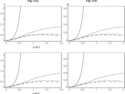
The profiles of the velocity u, w and temperature respectively for various values of time t and for couple stress parameter ∝����2 = q = 0.1, 0.5, 1.5, for y = o, s = 1, m =3 and for 𝜇𝜇=0.0, 0.05, and 0.1, have been computed, it is observed that increasing couple stress parameter decrease velocity and temperature in fig. 1(a), (b) and (c).

Fig 2(a) (b) and (c) shows the variation of the velocity components u and w and the temperature at the central plane of the channel (y = o) with time for various values of the Hall parameter m and 𝜇𝜇 = 0.0, 0.05, and 0.1, in these figures S = o, q = 0.5 in 2 (a), (b) shows that u, w increase with increasing ‘m’ for all values of 𝜇𝜇, but in fig. 2 (b) shows the influence of 𝜇𝜇 on w depends on t and more clear when m is large. It is observed that, increasing 𝜇𝜇 decreases w and increasing m increases w.

Figure 2 (c) and shows that the influence of m on 𝜃𝜃 depends on t. Increasing 𝜃𝜃 at small times but this is reversed at large times. This is due to the fact that, for small time u and w are small and an increase in m increases u but decrease

w then, Joule dissipation which is also proportional to � 1

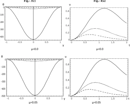
1+ 𝑚𝑚2� decreases. For large times increasing m increases both u and w and m turn, increases the Joule and viscous dissipations. This accounts for the crossing of the curve of 𝜃𝜃 with time for all values of 𝜇𝜇. It is also observed that increasing 𝜇𝜇 decreases the temperature both u and w their gradients which decreases the Joule and viscous dissipations. These figures shows also that the time at which 𝜃𝜃 reaches steady state value increases with increasing m while it is not greatly affected by changing 𝜇𝜇. Fig. 3 (a) (b) and (c) present the profiles of the velocity components u and w and the temperature 𝜃𝜃 for various values of time it and for 𝜇𝜇 = 0.0, 0.05, 0.1 the figures are evaluated for m = 3, s = 1, q = 0.5, it is clear from Figures 3 (a) (b) and (c) that effect of 𝜇𝜇 on u, w and 𝜃𝜃 depends on t and y. Figure 3 (a) shows, that, for small t, increasing the 𝜇𝜇 decreases u for small y but this is reverse for large y. As time develops increasing 𝜇𝜇 increases u for all y. Figure 3(b) & (c) shows that increasing 𝜇𝜇 increasing w for all values of y.

For large t, increasing 𝜇𝜇 decreases w and 𝜃𝜃 for small t and all values of y, this can be attributed to the fact that increasing 𝜇𝜇 will delay the attainment of maxima of u, w and 𝜃𝜃. It is also observed from figures 3 (a), (b) and (c) that the velocity components u, w and 𝜃𝜃 do not reach their steady state monotonically. It is observed also that the velocity component u reaches the steady state faster than w which, in turn, reaches the steady state faster than 𝜃𝜃. This is expected as u is the sources of w. while both u and w act as sources for the temperature.

Transfer of A Couple Stress Fluid / IJMA- 6(6), June-2015.

Fig. 4 (c) shows that the influence of a on 𝜃𝜃 depends on t. It is observed that increasing a decreases 𝜃𝜃 while it is not greatly affected by changing 𝜇𝜇. The figure shows also that the time at which𝜃𝜃 reaches its steady state value decreases with increasing a while it is not greatly affected by changing 𝜇𝜇.

Fig.5(a), (b) and (c) show the profiles of the velocity components u w and the temperature𝜃𝜃, respectively for various

values of time a and for t=0.2,1, and 2. The figures are evaluated for m=3,𝜇𝜇= 0.05 and s=1.It is clear from fig 5(a), (b) that the effect of decaying parameter a on u and w depend on t and y. Fig 5(a) (b) shows that for small t, increasing a decreases u, w for all values of y and a. It is also observed that increasing a decreases u for all values of y with significant difference at medium and large t. It is also observed that the constant pressure gradient a=0 is greatly different from unsteady pressure gradient. This can be attributed to the fact that increasing a will decrease the pressure gradient which mainly generates the velocity u. Fig 5(c) shows the temperature𝜃𝜃 profile does not reach its steady atate monotonically, increasing a decreases 𝜃𝜃 for all values of y and a. It is also observed that increasing a decreases 𝜃𝜃 for all values of y with no significant difference at medium and large t. It is also observed that the constant pressure gradient a=0 is greatly different from unsteady pressure gradient. This can be attributed to the fact that increasing a will decrease the pressure gradient which mainly generates the velocity u and w. This is expected as u is the source of w, while both u and w act as sources for the temperature.

CONCLUSION

A transform technique is used to save the transient coutte flow and heat transfer of a couple stress fluid under the influence of unsteady pressure gradient and uniform magnetic field. In the present work, we study Hall effect, couple stress parameter, the effect of the decaying parameter a and the Hall parameter m on the velocity and temperature distributions are studied. The decaying parameter a affects the main velocity components u and w and the temperature

𝜃𝜃. The Hall term affects the main velocity components u in the 𝜘𝜘 – direction and gives rise to another velocity component w in the z – direction.

The results show that the influence of the parameters a and 𝜇𝜇 on u and w depend on time and Hall parameter m. It is also found that the effect of m on w and 𝜃𝜃 depends on time for all values of 𝜇𝜇 which accounts for a cross over in the w-t and 𝜃𝜃-t graphs for various values of m. The effect of m on the magnitude of 𝜃𝜃 depends on 𝜇𝜇 and becomes more pronounced in case of small 𝜇𝜇. It is also found that the effect of a and q on the magnitude of 𝜃𝜃 depends on 𝜇𝜇 and becomes more pronounced in case of small 𝜇𝜇.

Fig.-1(a) Fig.-1(b)

u w

t

µ=0.1

t

µ=0.0

0 0.5 1 1.5 2

0 0.5

1 1.5

2 2.5

3

0 0.5 1 1.5 2

0 0.2 0.4 0.6 0.8

0 0.5 1 1.5 2

0 0.5

1 1.5

2 2.5

3

0 0.5 1 1.5 2

t

;_______q=0.5...q =1,______ a =1.5, _______q=0.5...q =1,____q =1.5

Fig.-1a, 1b, 1c: Effect of couple parameter q on u, w, θ at y=0 for various values of  m S=1)

Fig.- 1(c) Fig.- 2(a)

Θ u

t t

µ=0.5 µ=0.0

Θ u

t t

µ=0.1 µ=0.05

θ u

t t

µ=0.01 µ=0.1

;_______q=0.5...q =1,______ a =1.5, ______m=0.0...m =1,____q=2

Fig.-2(b) Fig.-2(c)

0 0.5 1 1.5 2

0 0.5

1 1.5

2 2.5

3

0 0.5 1 1.5 2

0 0.2 0.4 0.6 0.8

0 0.5 1 1.5 2

-250 -200 -150 -100 -50 0

0 0.5 1 1.5 2

-0.2 -0.15 -0.1 -0.05 0 0.05

0.1

0 0.5 1 1.5 2

-250 -200 -150 -100 -50 0

0 0.5 1 1.5 2

-0.2 -0.15 -0.1 -0.05 0 0.05

0.1

0 0.5 1 1.5 2

-250 -200 -150 -100 -50 0

0 0.5 1 1.5 2

Transfer of A Couple Stress Fluid / IJMA- 6(6), June-2015.

w θ

t t

µ=0 µ=0

w θ

t

µ=0.05 µ=0.1

Θ t

t t

µ=0.1 µ=0.1

;_______m=0...m =1,______ m =2, _______m=0...m =1,______ m =2

Fig.-2a, 2b, 2c: Effect of Hall curremt m on u, w, θ at y=0 for various values of µ ( a=3, S=0)

Fig.-3(a) Fig.-3(b) w u

y y

µ=0.0 µ=0.0

0 0.5 1 1.5 2

-0.6 -0.4 -0.2 0 0.2 0.4

0 0.5 1 1.5 2

-1.2106

-1106 -800000 -600000 -400000 -200000 0

0 0.5 1 1.5 2

-0.6 -0.4 -0.2 0 0.2 0.4

0 0.5 1 1.5 2

-50000 -40000 -30000 -20000 -10000 0

0 0.5 1 1.5 2

-0.6 -0.4 -0.2 0 0.2 0.4

0 0.5 1 1.5 2

-17500 -15000 -12500 -10000 -7500 -5000 -2500 0

-1 -0.5 0 0.5 1

0 0.2 0.4 0.6 0.8

-1 -0.5 0 0.5 1

0 0.05

w

Y y

µ=0.05 µ=0.05

w

Y y

µ=0.1 µ=0.1

;_______t=0.2...t =1,______t =2, _______t=0.2,...t =1,______ t =2

Fig. - 3a, 3b, 3c: The variation of time t on u, w, θ at m=3 for various values ofµ ( a=1, S=0)

Fig.- 3(c) Fig.- 4(a)

θ u

y t µ=0.0 µ=0.0

θ u

y t

µ=0.05 µ=0.05

-1 -0.5 0 0.5 1

0 0.2 0.4 0.6 0.8

-1 -0.5 0 0.5 1

0 0.05

0.1 0.15 0.2 0.25 0.3

-1 -0.5 0 0.5 1

0 0.2 0.4 0.6

-1 -0.5 0 0.5 1

0 0.05

0.1 0.15 0.2 0.25 0.3

-1 -0.5 0 0.5 1

-400 -300 -200 -100 0

-1 -0.5 0 0.5 1

-500 -400 -300 -200 -100 0

0 0.5 1 1.5 2

0 0.2 0.4 0.6 0.8

0 0.5 1 1.5 2

Transfer of A Couple Stress Fluid / IJMA- 6(6), June-2015.

θ u

y t

µ=0.1 µ=0.1

;_______t=0.2...t =1,______t =2, ______a=0.,...a =1,______ a =2

Fig.- 4(b) Fig. - 4(c) w θ

τ

µ=0.05; µ=0.05 w θ

t

µ=0.1; µ=0.1; w θ

τ

µ=0; µ=0;

_______a=0...a =1,______ a =2, _______a=0...a =1,______ a =2

Fig.- 4a, 4b, 4c: Effect of decaying parameter a on u, w, θ at y=0 for various values ofµ ( m=3, S=1)

-1 -0.5 0 0.5 1

-500 -400 -300 -200 -100 0

0 0.5 1 1.5 2

0 0.2 0.4 0.6 0.8

0 0.5 1 1.5 2

0 0.5

1 1.5

2

0 0.5 1 1.5 2

-600 -400 -200 0

0 0.5 1 1.5 2

0 0.5 1 1.5 2

0 0.5 1 1.5 2

-800 -600 -400 -200 0

0 0.5 1 1.5 2

0 0.5

1 1.5

2

0 0.5 1 1.5 2

Fig. -5(b) Fig.- 5(a)

w µ=0.05 u

y y

t=0.2 t=0.2

w u

y y t=1 t=1 t=1

w u

y y

t=2 t=2 t=2 ;_______a=0...a =1,______ a =2, _______a=0...a =1,______ a =2

Fig.- 5a, 5b, 5c: Effect of decaying parameter a on the distribution of u, w, θ with y for various values of t (µ=0.05, m=3, S=1)

Fig.- 5(c)

θ θ

y

t=0.2 t=1

-1 -0.5 0 0.5 1

0 0.05

0.1 0.15 0.2

-1 -0.5 0 0.5 1

0 0.02 0.04 0.06 0.08

-1 -0.5 0 0.5 1

0 0.5

1 1.5

2

-1 -0.5 0 0.5 1

0 0.2 0.4 0.6 0.8

-1 -0.5 0 0.5 1

0 0.2 0.4 0.6 0.8 1 1.2

-1 -0.5 0 0.5 1

0 0.1 0.2 0.3 0.4 0.5

-1 -0.5 0 0.5 1

-700 -600 -500 -400 -300 -200 -100 0

-1 -0.5 0 0.5 1

Transfer of A Couple Stress Fluid / IJMA- 6(6), June-2015.

y

y t=2

Fig.-5a, 5b, 5c: Effect of decaying parameter a on the distribution of u, w, θ with y for various values of

t (µ=0.05, m=3, S=1)

REFERENCE

1. I.N. Tao. J- of Aerospace Sci., Vol. 27, 1960. PP. 334 – 347.

2. S.D. Nigam and S.N. Sigh, The Quarterly Journal of Mechanics and Applied Mathematics, Vol. 13, 1960. PP. 85 – 97.

3. R.A. Alpher. International Journal of Heat and mass transfer, Vol. 3 No. 2, 1961. PP. 108-112. 4. I. Tani Journal of Aerospace Science, Vol. 29, 1962. PP. 287 – 296.

5. G.W. Sutten and A Sherman, Engineering Magneto hydrodynamics, Mc Graw-Hill, New York. 1965. 6. V.M. Samdalgekar, N.V. Vighnesam and H.S. Takhar ,EEE Transactions on plasma Science. Vol. PS-7, No. 3

1979, PP. 178 – 182.

7. V.M. Soundalgekar and A.G. Uplekar. EEE transactions on plasma Science. Vol. PS – 14, No. 5. 1986. PP. 579 – 583.

8. E.M.H Abo-EL-Dahab, “Effect of Hall current on some Magneto hydrodynamic flow problems”. Master thesis Helwan University. Am Helwan, 1993.

9. H.A. Attia and N.A. Kotb. Acta Mechanica, Vol. 117, No. 1-4. PP. 215 – 220, 1996. 10. Stokes, V.k. The physics of fluid 3 (9) PP. 1709 – 1715. 1966.

11. Singh and Pathak, Ind., Jo of pure and Appl. Math 8(6) PP. 695 – 701. 1977. 12. Rathod V.P. and Parveen S.R. Math Edn. 3, PP. 121 – 133 (1997).

13. Gudiraju, M., Peddieson, J. and Munukutle. S. Mechanic Research communication 19, PP 7 – 13. 1992. 14. Dube, S.N. and Sharma, C.L., J. Phy. Soc. Japan 38. PP. 298 – 310 (1975).

15. Ritter. J. M. and Peddieson J. Proceeding of the 6th Canadian Congress of Applied Mechanics (1977). 16. Chamkha, A.J. Mechanic Research Communication, Vol. 21 (3) PP. 281 – 286 (1994).

17. Rathod V.P. and Baderunnisa Begum. Int. J. Mathematical Science and Engineering Application 4 (4) PP. 229 – 241. 2010.

18. Rathod V.P., Patel G.S. and Haq K.A. Sci. and Tech. Res. J. GuG. 3, (1990).

19. Rathod V.P. and Syeda Rasheeda Parveen. Int. J. Mathematical Science and Engineering Application Vol. 8 No. 11, 149 – 160. 2014.

20. Rathod V.P. and Syeda Rasheeda Parveen Int. J. Mathematical Science and Engineering Application Vol. 8 No. IV 189 – 194, July – 2014.

21. Rathod V.P. and Syeda Rasheeda Parveen. IJMA Vol. 6 No. 3 PP. 11 – 18 2015.

22. E.Rukmangadachri. “Dusty Viscous flow through a cylinder of Rectangular Cross – section under time dependent pressure Gradient”. Defense Science Journal, Vol. 31, No. PP. 143 – 153. 1981.

23. M.E. Sayed Ahmed. Hazeem. A. Attai and Karem M. twis “Time dependent pressure Gradient effect on unsteady MHD Couette flow and heat transfer of a caisson fluid. Engineering. 3 PP. 38 – 49. 2011.

24. H.A. Attia. “Hall Current effects on the velocity and temperature fields of an unsteady Hartmann flow”. Canadian Journal of Physics Vol. No. 9, PP. 739 – 746. 1998.

25. Sneddon I.N. “Fourier Transforms”. Mc. Graw-Hill Book. Co-New York. 1951.

Source of support: Nil, Conflict of interest: None Declared

[Copy right © 2015. This is an Open Access article distributed under the terms of the International Journal of Mathematical Archive (IJMA), which permits unrestricted use, distribution, and reproduction in any medium, provided the original work is properly cited.]

-1 -0.5 0 0.5 1