Vol 8, No 6 (2017)

(1)

International Journal of Mathematical Archive-8(6), 2017,

253-264

Available online throug

ISSN 2229 – 5046

WEAK – WAVES IN GAS PARTICLE MIXTURE

**KANTI PANDEY*, DEWKI NANDAN TEWARI**

Department of Mathematics & Astronomy, Lucknow University, Lucknow 226007, India.

Received On: 30-05-17; revised & Accepted On: 15-06-17)

ABSTRACT

I

n present paper an attempt has been made to discuss weak – non -linear waves in gas particle mixture for a binary dissociated gas when particle volume fraction is negligible and equilibrium is eventually established. Equation of motion, wave and weak shocks are discussed. Applying method of linearization compatibility condition, relatively undistorted wave condition and shock formation is obtained. For high frequency harmonic wave asymptotic analysis is applied to obtained the solution up to second order. Variation of velocity is interpreted through graphs for various values of density, specific heat of mixture and rate of internal change. In preparation of graphs Mathematica 7 is used.

Classification: 76 T, L.

Key words: (Weak –Waves /gas –particle mixture).

1. INTRODUCTION

Equation of state with one rate dependent state variable arises in the study of gases subject to chemical dissociation or vibrational relaxation. In the former case the possible effects of diffusion are normally neglected so that the purely chemical phenomenon is treated in isolation. Comprehensive review articles in this field and its applications have been written by Lick [8]. The propagation of disturbances, governed by non linear hyperbolic systems, may exhibit a distortion of wave profile. This was studied by Varley and Cumberbatch [20], Dunwoody [4], Parker and Seymour [15] by using theory of relatively undistorted waves as an extension of the idea of Courant and Hilbert [2] for linear-waves. Sharma et.al [19] have considered non linear wave propagation in a hot- electron plasma by using theory of relatively undistorted wave. They have used a simple asymptotic expansion method to calculate first and second order solutions.

The studies of non-linear effects on the wave propagation have been extensively carried out by Jeffery and Taniuti [7], Whitham [23], Courant and Friedrichs [3]. If the amplitude of the disturbance is not sufficiently small, the wave form is also altered by non-linear effects during propagation. Vincenti and Kruger [22], Chu [1] have formulated the general non linear equation for the relaxing gas flow and studied the effects of relaxation on acceleration-wave during propagation and their termination into a shock wave. Parker [16] has considered the effect of non linearity and relaxation on the propagation of a one dimensional wave.

By two-phase flows we mean a special flow problem in which we consider the mechanism of two – phases of matter simultaneously. In general two-phase flows may be divided in two groups. The first group consists of flow problems of mixture of two-phases of four states – solids (pseudo – fluid), liquid, gas and plasma, where two-phases may be mixed homogeneously or in-homogenously. In second group of flow problems, interaction between the two-phases of matter through their interface is important. In present article we consider first group of two-phase flows neglecting particle interaction, which has its importance in internal ballistic, lunar ash flow, exploding wire phenomena, under water explosion, astrophysics (explosion in stars), atmosphere of earth etc. There are many engineering problems in which dilute phase of gas – particle is a good approximation of actual conditions. In such cases due to the existence of solid particles in the gas, properties of mixture differ significantly from those of gas alone. Such types of studies have numerous application in underground explosions [9, 10]. The study of wave propagation in a mixture of gas and dust particle has received great attention during several years. There are many engineering application for flow of suspension of powdered material or liquid droplets in a gas. Dusty gas flow assume importance in such engineering problem as flow in rockets, nuclear reactors, fluid sprays, air pollution, medicine etc. Propagation of rapid pulses though a two phase mixture of gas and dust particles, when particle volume fraction is negligible is studied by Gupta

et. al. [5] However they have used second order solution to describe the far field behavior of weak shock. In this context following references can be cited [6, 11-14].

Corresponding Author: Kanti Pandey*

(2)

© 2017, IJMA. All Rights Reserved 254 In present analysis, we consider the case of two – phase flows of solid particles (which are spheres of identical mass, radius, and specific heat) for negligible particle pressure and particle volume – fraction (the case of moderate particle loading). Equation of motion, wave condition and its termination in to shock wave is considered. Using asymptotic analysis solution up to second order is obtained.

2. EQUATION OF MOTION

Following Rudinger [18] and Vincenti and Kruger [22] equations governing one dimensional motion of gas particle mixture for a binary dissociated gas, when particle volume fraction can be neglected and equilibrium is eventually established is given by

,t

u

,

x

u

,x

0,

ρ

+

ρ

+

ρ

=

(2.1)

(

,

)

,

0,

1

x t x

p

u

uu

η ρ

+

=

+

(2.2)

(

)

₍

₎

(

)

(

)

,

0

1

1 ,

,

1

,

, , ,

, ,

,

=

+













+

−

+













+

−

+

x x

p

x t

t p

t

uH

p

H

u

uH

H

p

H

α

ρ

η

ρ

η

α

ρ

η

ρ

η

α

ρ α

ρ

(2.3)

0 )

,

(

,

+

α

+

ρ

α

=

α

_t

u

_x

f

p

_m (2.4) where

ρ

_m

=

(

1 +

η

)

ρ

,

ρ

being density of gas and

η

the mass flow ratio, u and p being gas velocity and gas pressure respectively.

H

=

H

(

p

,

ρ

m

,

α

)

is the enthalpy of mixture and

α

is rate of dissociation. Comma followed by an

index denotes partial differentiation with respect to that index.

Equation (2.1) to (2.4) can be rewritten in the following matrix form

0 ,

,

+

BU

+

C

=

AU

_t _x (2.5) where A, B are 4x4 matrix and U & C are column vectors which can be obtained from equation (2.1) to (2.4) by inspection. Here we will consider the propagation of waves into an equilibrium state defined at a point

(

p

0

,

ρ

m₀

α

0

)

_,

given by

0 )

,

(

p

₀

v

₀

α

₀

=

f

(2.6)

where

m

v

ρ

1 =

which is said to be asymptotically stable at constant pressure and volume if the solution

α

(

t

)

of

(

0

,

0

,

α

0

)

α

v

p

f

Dt

D

₌

₋

,

α

( )

0 =

α

∗ (2.7)

exists for all t˃0 and α(t)→α0 as t→0 for all α

∗

such that

−

0

<

,

>

0 .

∗

_α

_ξ

α

Following thermodynamic properties given by Dunwoody4 we have

2

,

1

f

m

a

H

α

d

γ

=

+

−

where

2

,

m f

m

p

a

γ

ρ

=

ξγη

ξη

γ

+

=

1

m is the ratio of specific heats for the mixture,

,

p

c

ξ =

c the specific heat of particle, d the heat of

reaction.

A ‘wavelet’ is defined by the curve

φ

=

φ

(

x

,

t

)

and if we assume that

0,

t

ϕ

∂

_≠

∂

then

t

=

T

(

x

,

φ

)

is equivalently.

By using transformation of co-ordinates (x, t) to (x,

φ

) any vector valued function

χ

transforms as

( , ( , ))

x T x

U x

( , )

χ

φ

=

φ

. (2.8)

Condition for relatively undistorted wave is defined by the relation

x x

(3)

where

.

denote the Euclidean norm of a vector. Since

x x x

x

T

U

_,

=

χ

_,

+

_,

χ

_, , (2.10) from equation (2.9)

χ

_,_x

≅

−

T

_,_x

χ

_,_t. (2.11)

Equation (2.10) hold exactly at an acceleration wave- front propagating into an undisturbed region in thermodynamic

equilibrium. On all other wavelets in a non dissipative gas

U

_,_x

=

0

i.e.

χ

(

x

,

T

(

x

,

φ

))

=

U

(

φ

)

is a solution.

The equation (2.5) may be written as

(

BT

,x

−

A

)

χ

,t

=

BU

,x

+

C

,

(2.12)

Thus equation (2.9) and (2.11) are compatible if

,

(1).

x

C

O

BU

=

.

(2.13)

As

det(

B

−

W

−1

A

)

=

0 ,

where

W

=

T

_,_x_(2.14)

1

−













∂

x

T

is an eigenvalue of

B

A

−1and the wavelets are the characteristics of (2.5). Thus

χ

must satisfy the

compatibility condition

(

,x

)

0,

l BU

+

C

=

(2.15)

where

l

is the left eigenvector associated with the eigen value

W

−1

.

As conditions (2.9) and (2.13) may be satisfied at a near equilibrium state, to the first approximation

(

BT

,x

−

A

)

U

,ϕ

=

0

. (2.16)

The solution of det.



_

B W

−

−1

A



_

=

0 



gives the Eigen value

1 1

,

f

T

W

u

a

x

− −

∂



_{ =}

_{= +}



_∂







(2.17)

where

a

_f local speed of sound and is given by

(

)

.

1

,













+

−

=

ρ

η

ρ

p f

H

a

The left Eigen vector associated with Eigen value (2.17) is given by

(

)

(

)

{

1 , , 1

f

, ,

f

,

f

,

}

.

l

=

+

η ρ

H

ρ

+

η

a H

ρ

−

a a H

α (2.18)

When equation (2.17) is substituted in equation (2.15) on integrating the resulting equation we have the solution to a plane wave propagating into a region which is in thermodynamic equilibrium given as

(

)

1 1

2 2

0 0

2 ,

,

1

m m

m

p

u

γ γ

γ

α α

ρ

η γ

− −





=

_

−

_

+

_{− }

_

2 1 2 1

1

−

+

=

_m m

f

a

γ

ρ

γ

η

(2.19) Here

ρ

₀

,

p

₀

,

α

₀are the values of the state variables on the leading characteristics.

3.RELATIVELY UNDISTORTED APPROXIMATION

Since (2.19) gives the relation between u,

ρ

,

p

and

α

then substituting equation (2.18) into equation (2.15) we have

(

)

,

( , , )

0. 2(

)

1

f x

f

a

H

u

f p

u

a

H

α ρ

ρ α

η ρ







+

_

_

=

(4)

(

)

(

)

1 1 2 2 0

2

1

1 ,

2

1

m m m f m m

u

a

γ γ

γ

ρ

η γ

− −





+

=

_

+

−

_

+

_{− }

_

(3.2)

(

)

1

,x f

.

T

=

u

+

a

− (3.3)

Using following linearization

0 0

,

0 0 0

0

p

u

a

f

a

f

a

f

p

=

+

′

ρ

=

ρ

+

ρ

′

α

=

α

+

α

′

=

+

′

=

+

′

(3.4)

Equation (3.1) and (3.3) reduces to

(

)

( )

₀

_{( )}

0

( )

2

, ₀ , ₀

, , ₀

, ₀

1 0,

2 1

p f x f

f

a

f

u

H

u

a

H

ρ α ρ

η



+





′

−

_

_

′

=

+

_

_

_

_

(3.5)

and 0 1 , 0

1

1 .

2

m x f f

T

a

u

a

γ

−





+

_′





=

_

−

_







(3.6)

Integrating equation (3.5) we have

) (

)

(

− − ∗

=

′

x x

e

g

u

ϕ

λ (3.7)

where

(

)

( )

_



_









+

=

, ₀

0 , 2 0 , 2 0 . 0 0

1

2

1

α ρ ρ

η

λ

H

a

f

a

f

f f p

and

g

(

φ

)

=

u

′

(

x

∗

,

t

)

i.e.

φ

is the time that a wavelet leaves the station

x

∗, where λ will be positive. On

substituting (3.7) in (3.6) and integrating the equation of any wavelet,

φ

=

constant, is obtained as

(

)

(

1 )

2

1 )

(

)

(

( )

0



−













₊

+

−

=

−

∗ − x−x∗

f m f

e

a

g

x

T

a

o λ

λ

γ

ϕ

. (3.8)

The formation of shock wave is characterized by

T

_,_x

=

0 .

Differentiating equation (3.8) with respect to

φ

we get

(

( )

)

, , 2

1

1 ( )

1

0.

2

o

x x m

f

T

g

e

a

λ ϕ ϕ

γ

ϕ

λ

∗ − −



₊



= +



_



_

− =





(3.9)

Differentiating equation (3.7) partially with respect to t we get

( )

, , ,

.

x x

t T

u

′ =

g

_ϕ

ϕ

e

−λ −∗ (3.10)

Putting the value of

φ

_,_Tfrom equation (3.9) in to (3.10) we get (taking

φ

=

0

)

1

( ) ( )

, 0 , 0 2 ,

0

1 (

)

{

( )}

1 (0){

1}

.

2

x x x x

m t

f

u

g

e

a

λ λ

φ ϕ ϕ ϕ

γ

ϕ

λ

∗ ∗ − − − − − = =



₊





′

=

_

+

−

_







(3.11)

The relatively undistorted approximation is valid if

φ λ

φ

γ

_ϕ

λ

ϕ

φ

, ) ( 0 ,

)

(

2

1

1 )

(

)

(

0

T

e

g

a

g

_x _x

f m f

















₊

+

≥

₋ ₋ ∗ (3.12)

which is satisfied automatically at a wave front

ϕ

=

0

where g(0) = 0 or near a shock wave

T

_,_φ

=

0

. It is also satisfied in the degenerate case of (

λ

0

f

(5)

At

x

=

x

∗

=

0 ,

T

_,_φ

=

1 .

This approximation is valid if local frequency is given

( )

,

, 0 0

( )

.

( )

L f f

g

T

a

g

ϕ

ω

λ

ϕ

=

≥

=

(3.13)

The validity of approximation may be extended to all values of

(

x

,

ϕ

)

provided

1 )

(

,

)

(

0

2 0 ,

≤

f

a

g

M

a

g

φ

λ

ϕ

φ

(3.14)

where M is finite.

The condition is also satisfied by small amplitude high-frequency sound waves i.e. frequency is high in a sense relative to natural time

(

a

f₀

λ

)

−1.

Relations (3.13) suggest a parameter for an asymptotic analysis.

4. WEAK SHOCK WAVE

The behavior of a dissipative gas through a shock is exactly similar to that of its non-dissipative counterpart. In particular the relations

[ ]

α

=

0

,

[ ]

S

≥

0

, where S is entropy and brackets denote the discontinuity in a variable across the shock must hold. For weak shock the entropy jump is of third order in the density jump, while to a first approximation, the shock speed U is that of the local resulting speed of sound i.e.

U

≅

a

_f.

In the limit of weak shocks the relation (2.19) satisfy compatibility conditions i.e. the jump in any variable for two values of

φ

say

φ

₁and

φ

₂coalesce at a shock. From equation (3.7)

[ ]

{

( )

}

( )

1 2

.

x x

u

=

g

ϕ

−

g

ϕ

e

−λ − ∗ (4.1)

The speed of shock surface G is given by

(

1 1

) (

2 2

)

1 .

2

f f

G

=

_



a

′

+

u

′

+

a

′

+

u

′



_





(4.2)

To a first approximation and through equation (3.3) the relation

{

}

1 ( )

0 1 2

0

1

1 ( )

(

)

.

4

x x m

f

a

g

e

G

a

λ

γ

_ϕ

∗

−





+

− −





≅

_

−

+

_







(4.3)

At the shock

t

₁

=

t

₂and

x

₁

=

x

₂where

(

x

₁

,

t

₁

),

(

x

₂

,

t

₂

)

are the coordinates of a point on

φ

₁ and

φ

₂respectively. From equation (3.8) putting values of these coordinates we get

{

( )

}

1 2

1 2 0

1 1 .

( )

(

)

2

x x m

f

e

g

a

λ

γ

ϕ ϕ

ϕ

λ

∗

− −

+

−

_{= −}

₋

−

(4.4)

In general characteristics have the explicit form

)

(

)

,

(

x

f

t

=

φ

+

φ

_(4.5)

and any curve interested by these curves may be represented in (x, Ф) coordinates. Since shock will be described by a

curve t=s(x) it follows from equation (4.5) and the implicit function theorem that along the shock

)

(

x

ψ

φ

=

_{. (4.6)}

From equation (4.5) and (4.6)

)

(

))

(

,

(

x

f

t

=

ψ

+

ψ

and from equation (4.5) and (3.8)

( )

₍

₎

















−

+

















₊

−

≅

=

− − −∗ − −∗

dx

d

g

e

a

e

g

a

dx

x

dS

G

x x

f m x

x

f m f

φ

λ

γ

φ

γ

φ λ

λ

)

(

1

2

1

1 )

(

2

1

, ) ( 2 )

(

0 1

0

(6)

(

)

{

}

{

}

dx

d

g

dx

d

g

2 1 2 1 , 2 2

1 2 1 1 , 2

1

)

(

)

(

)

(

)

(

)

(

)

(

)

(

φ

−

φ

−

_φ

φ

−

φ

=

φ

−

φ

−

φ

−

φ

_φ

φ

_(4.8)

{

}

0 0

( ) ( ) 2

2 , 2

2 2

1

1 (

)

1 (

)

1

0 .

4

2

x x x x

m m

f f

d

g

e

g

e

a

dx

λ λ

ϕ

γ

_ϕ

γ

_ϕ

ϕ

λ

∗ ∗

− −



− −



+



+



−

+ +

_

−

_

=







(4.9)

As Ф1 = 0, after integration we have

0

2

1

4

m

f

a

γ

λ

+

_{

_}

2

( )

2 2 0

( )

1

2 (

)

x x

g s

e

ds

g

ϕ λ

ϕ

∗

− −

_{− =}

∫

(4.10)

and as Ф2→0 we find

{

}

2

1

0 2 ,

2 0

( )

lim

2 (0)

.

(

)

g s ds

g

ϕ

_ϕ

ϕ

−

→

∫

=

_(4.11)

At the shock

_∂

=

0 ,

∂

x

T

and

(

)

0

1/ 2 ( )

2

1 (

)

1 .

2

x x m

f

g

e

a

λ

γ

ϕ

λ

∗

− − −



₊





∝ −

_

−

_







(4.12)

[ ]

(

)

0

1/ 2 ( ) 2 ( )

1

2

x x x x m

f

u

e

a

λ λ

γ

λ

∗ ∗

− − − −



₊





∝ −

_

−

_







(4.13)

The distance by which the shock is ahead of the zero wavelet

0 0

s

x

t

=

φ

+

_{increased by an amount}

(

)

0

1/ 2 ( ) 2

1

1 .

2

x x m

f

e

a

λ

γ

δ

λ

∗

− −



₊





∝

_

−

_







(4.14)

In limit λ→0, all the above results reduce to those obtained by Whitham [23].

5. ASYMPTOTIC ANALYSIS

In this section we consider the propagation of high frequency harmonic wave. At x = 0 the initial conditions are taken to be

β

ω

β

σ

ω

β

σ

ω

2 1 1

,

sin

),

cos

1 (

− −

−

₋

₌

=

u

t

x

_{. (5.1)}

So, that a given wavelet is described by β=constant and the conditions (3.13) and (3.14) are seen to be satisfied for

1

0

≥

λ

ω

f

a

,

σ

being the maximum acceleration and is finite, the transformation in this case becomes

)

:

,

(

x

β

ω

T

t

=

_{, (5.2)}

thus boundary condition is given by.

.

sin

)

(

1

0 2 1

,β

ω

σ

β

− −

−

₋

₊

=

a

u

T

_f _(5.3) In terms of characteristic co-ordinates the equations (2.16) and (2.17) becomes

(

B T

ij ,x

−

A

ij

)

U

j,β

=

T

,β

(

B U

ij j x,

+

C

i

)

_{, (5.4)} 1

,x

(

f

) .

(7)

Conditions (5.1) and (5.3) suggest that we can now consider asymptotic expansion of the form

),

,

(

1

β

x

u

n N n n

∑

=

∈

=

∑

=

∈

+

=

N n n n

x

p

1

0

(

,

β

)

0 1

( , ),

N n n n

x

ρ ρ

ρ

β

=

+

∑

∈

(

,

)

1

0

a

x

β

a

N n f n f

f

∑

_n

=

∈

+

=

_(5.5)

∑

=

∈

+

=

N n n n

x

T

x

T

1

0

(

)

(

,

β

)

(

,

)

1

0

α

β

α

x

N n n n

∑

=

∈

+

=

)

,

(

1

0

f

x

β

f

N n n n

∑

=

∈

+

=

the constant appearing in (5.5) are the equilibrium values of the respective variables

∈=

ω

−1

,

where successive terms

such as Un and Un+1 have the ratio 0

1

(

).

n f n

U

O a

U

₊

=

λ

In similar way asymptotic expansion for each Eigen value is given by

n n n n

l

∑

=

∈

+

=

1

0 _(5.6)

and on any characteristic curve the relations

(

,x

)

,x

l BT

−

A U

=

l BU

(

_,_x

+

C

)

=

0

_(5.7)

must hold.

Equation (5.4) and (5.7) form the basis of the approximating scheme.

Zeroth Approximation

Substituting equation (5.5) in equation (5.4), (2.18) and equating constant terms (i.e. zeroth power of ∈) 𝑓𝑟𝑜𝑚 both sides, we have

0 0,

1 ,

x f

T

a

=

(5.8)

(

₀ ₀_, ₀

)

0

B

T

−

A

=

l

_x

.

(

)

( )

(

)

( )

{

0 0 0

}

0

1

0 , ₀

, 1

f , ₀

,

f

,

f , ₀

,

l

=

+

η ρ

H

ρ

+

η

a

H

ρ

a

H

α (5.9)

where 0 0 f

a

x

T

=

is appropriate boundary condition

First approximation: Proceeding exactly in similar ways as done for zeroth approximation for first and second approximation we have following results

(

)

(

)

{

}

{

}

{

}

0 .

,

0 ,

) 0 ( , 0 ) 0 ( ) 1 ( ) 1 ( , 0 ) 1 ( , 1 ) 0 ( ) 0 ( ) 1 ( , 1 ) 0 ( ) 0 ( 1 , ) 0 ( 0 ) 0 ( 1 2 ,

1 ₀ ₁

=

−

+

−

+

=

+

=

−

+

−

=

− ij x ij i ij x ij x ij i i j ij i j ij ij f f x

A

T

B

l

A

T

B

T

B

l

C

U

B

l

u

A

T

B

a

u

a

T

β β (5.10)

From first three equations of (5.10) and the appropriate boundary conditions

u

₁

=

σ

sin

β

,

T

₁

=

β

,

we have

{

}

1

sin

exp

(

) ,

u

=

σ

β

−

λ

x

−

x

∗ .

{

}

0 0 ( ) 1

1 (

)

sin

1

2

x x m

f

a

T

e

a

λ

γ

β

σ

β

λ

∗

− −

+

(8)

t

cons

u

a

u

a

p

f

tan

,

)

1 (

1

1 0 1

0

=

+

=

α

ρ

η

(5.12)

(

)

( )

(

)

( )

(

)

( )

0 1

1 1 0

0 , ₁ 1 , ₀ , ₁ , ₀

(1)

, ₀ , ₁

1

1 , 1

(1

)

,

f f

f f f

H

a

H

a

H

a

H

a

H

ρ ρ ρ ρ

α α

η ρ

η



₊

_{+ +}

₊

_{+ +}





= 



−

+









(5.13) Through equation (3.9) it is implied that shock will occur on all wavelets for which

g

_,_β

(

β

)

is maximum i. e on

𝛽= 2𝜋𝑛(𝑛= 0,1,2,3 … … . . ) and is first located at

















+

−

=

σ

γ

λ

(

1 )

2

1 log

1

2₀

m f

a

x

. (5.14)

Equation (4.3) shows that shocks formed on

β

=

2 π

n

,

(

n

=

1 ,

2 ,...

)

propagate with speed of sound and so a constant distance apart. The leading shock however moves ahead of that on

β

=

2 π

as indicated by equation (4.14). Any two wavelet

β

=

2 n

π

+

φ

and

β

=

2 n

π

−

φ

coalesce with the shock at the same instant and the substitution

φ

σ

ω

β

)

(

)

sin

(

₂

=

−

g

₁

=

−1

g

(5.15)

satisfies equation (4.7). Equation (4.4) shows that these two wavelets reach the shock where

0

2

1

2

m

f

a

γ

λ

+

_{

₍ ₎

_}

1 sin

x x

e

λ

ϕ

σ

ϕ

∗

− −

_{− = −}

(5.16)

Therefore it is implied by (5.16) and (4.1) that the strength of these shocks (𝛽= 2𝜋𝑛,𝑛= 1,2,3, … … ) decays like

[ ]

.

1

( )

) (

∗ ∗

− −

−

∝

x x x x

e

u

λ λ

Those wavelets𝛽 which lie in the region

2n𝜋+∅<𝛽< 2𝑛𝜋 − ∅ (n = 1, 2…….)

Never coalesce with a shock and so form the expansion regions separating the shocks.

Second Approximation: For second approximation

(

)

1

2 0

0

2

1 2

2, 2

(

)

,

f

x f f

f

u

a

T

a

u

a

−



+





=

_

−

+

_







(5.17a)

( )

{

(0) 0

}

( )2

{

(0) (1) (1)

}

( )1

(

(0) ( )1 (1)

)

0, , 1, 0, , 1, ,

ij x ij j ij x ij x ij j x ij j i

B

T

−

A

U

= −

B

T

+

B T

−

A

U

+

T

B

U

+

C

(5.17b)

( )

{

2

}

{

( )1

}

(0) (0) (2) (0) (1) (1) (1) (0) (1)

, , ,

i ij j i i ij j i ij j i

l

B

U

+

C

= −

l

B U

−

l

B

U

+

C

(5.17c)

while the remaining equation for

l

(2)is not considered.

With help of equation (5.11), (5.12), (5.13) we have

(

)

{

}

0

0 0 0

2

2 ₀ 2 , ,

0

1

1 ( )

( )

,

(1

)

2

s s s

m m

f

f f f

p

u

a

g

r e

g

r e

g r e

dr

a

β _λ _λ _λ

ϕ ϕ

γ

λ

η

ρ

λ

− − −



₊





− +

=

−

_

+

− +

_

+

∫

_

_

_

_

(5.18a)

where

( )

sin ,

g

β

=

σ

β

0

2 1

0 0

( , )

f

(1

)

_f

f

( )

s

,

f s

a

g

e

when

r

p

λ

β

η

β

ρ

−



_

_∂

_

_

_∂

_





=

_

_

_

+

_

_

_

=

∂













(9)

(

).

s

=

x

−

x

∗

(

)

0 0 0

0

2 2 ₀ 0 2 , 2 0 ,

1

3 [

1 ( )

] ( )

,

2

s s s

m m

f f f

u

g

r e

g

r e

g r e

d r

a

β _λ _λ _λ

ϕ ϕ

ρ

₋

_ρ

₌

₋

_{ρ λ}





₊

γ

+

−

₋





₊

γ

−

_ρ

− −











∫

(5.18b)

(

)

0 0

0

2 2 , 1

0

1

1 ( )

1 ( , )

,

2

s m

f f

g

r e

f s r dr

a

β

λ ϕ

ρ

γ

α

λ

−



₊





=

_

+

−

_







∫

(5.18c)

The arbitrary functions of x which arise in the integration are zero as the functions

u

₂

,

ρ

₂

,

p

₂and

α

₂are zero on

0 =

β

the leading characteristic for all x.

α

₂ is independent of the others but dependent in its behavior on what has occurred on the precursor wavelets. Thus, on integrating (5.18c), we have

( )

(

)

( )

{

0

}

(

)

0 0

2 2

0

2 , 0 , 0 2

1

1 ( )

4

s m s

p f

f f o

f

a

f

e

g

e

g r dr

a

β

λ λ

ρ

γ

α

η

β

λ

−





+

−





=

+

_

− +

_





∫



(5.19) and it is seen that at the piston

x

=

x

∗ the degree of internal excitation induced is

∫

∝

β

α

0

2

g

(

r

)

dr

, (5.20)

which is out of phase with the velocity wave. Its period is twice that of velocity and its effects is to induce frequency in the velocity wave.

From equation (5.17c) and (5.18a) after certain manipulation we have

(

)

2 ( ) ( )

2 2

0 0

1

x x x x

f

u

p

Ae

Be

Cx

a

λ λ

η

ρ

∗ ∗

− − − −

+

=

−

+

. (5.21)

and

(

)

2 2

2

0 0

,

1

s s

f

p

u

De

Ee

a

λ λ

η

ρ

− −

− +

=

+

(5.22)

where

s

=

(

x

−

x

∗

)

(

)

{

}

(

)

( )

(

)

2 ₂ 2

,

0 1

2 2

0 , ₀ 0

1 ( )

5

1

4 ₁

m

f

H

g

A

a

H

ρ

η ρ

β

γ

ρ

η





+





=

−

+



+







( )

(

)

( )

, ₁

,

0 0 2 ₀ ₁

0 0

, ₀ , ₀

1

1 ( )

1

2

f _m

f

H

a

_f

B

g

a

H

ρ

α

ρ ρ

λ

ρ

_γ

β

η ρ

ρ









+





_



_



−



_

_



=

_

+ +

−

_













(

)

( ) ( )

{

, ₁ 1

( )

, 2

}

0

, 0

1

1 f

H

f

H

C

_ρ _α

ρ

η

+

=

,

(

)(

)

2

0

1

1 ( ),

4

m

f

D

g

a

η γ

β

+

=

2 0

0 0

1 ( )

( )

4

m f

f

E

a

g r dr

g

a

β

_γ

λ

+

β

=

∫

−

.

From equation (5.21) and (5.22) we have

(

)

(

)

[

A

D

e

B

E

e

C

x

]

u

2

=

−

−2λs

−

+

−λs

−

(10)

6. RESULTS AND DISCUSSION

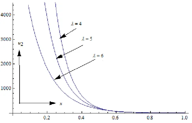
We have discussed the weak non-linear waves in gas particle mixture for a binary dissociated gas when particle volume fraction is negligible and equilibrium is eventually established. Equation of motion, wave and weak shocks are discussed. Applying method of linearization compatibility condition, relatively undistorted wave condition and shock formation condition is obtained. With the help of asymptotic analysis solution up to second order is obtained. Through first approximation shock formation and its decay behavior is investigated. During second order approximation velocity and rate dissociation is obtained. Variation of velocity is interpreted through graphs for various values of density, specific heat of mixture and rate of internal change. In preparation of graphs Mathematica 7 is used.

Figure-1: Variation of wave velocity for

λ

during first approximation.

(11)

Figure-3: Variation of wave velocity for different values of

λ

in second approximation.

Figure -4: Variation of wave velocity for different values of rate of internal state variable for second approximation.

(12)

ACKNOWLEDGEMENT

One of the author kanti pandey is grateful to UGC for providing financial assistance in preparation of this paper.

REFERENCE

1. Chu, B.T. –Non – Equilibrium Flow – Vol. 2, (Ed. P. P. Wegner), Marcel Dekker, Inc., (1970). 2. Courant, R. and Hilbert, D. - Method of Mathematical Physics, Interscience, New York, (1952). 3. Courant, R. and Friedrichs, K. O. - Supersonic flow and shock-waves, Interscience- New York, (1948). 4. Dunwoody, J. - High-frequency of sound waves in ideal gases with internal dissipation, J. Fluid Mech., vol.34,

pp. - 769-782, (1968).

5. Gupta, N., Sharma, V.D., Sharma, R.R. and Pandey, B.D. - Propagation of rapid pulses through a two- phase mixture of gas and dust particle, Int. J. Eng. Sci., Vol. 30, pp. 263-272,(1992).

6. Jena, J. and Sharma, V.D. - Self- similar shocks in a dusty gas, International Journal of Non- Linear Mechanics, Vol., 34, pp.- 313-327, (1999).

7. Jeffery, A. & Taniuti, T, - Non-linear Wave Propagation, Academic press, New York, (1964). 8. Lick, W. - Advances in Applied Mechanics, Vol. 9, Acadeemic Press, New York, (1967).

9. Mc queen, R.G. - Shock waves in condensed media, Eliezer, S. and Rice, R.A. (Eds.), High pressure equation of State Theory and Applications, North- Holland, Amsterdom, (1991).

10. Nagayama, K. - Shock wave interaction in solid material, Sawaoka, A.B. (Ed.), Shock Wave in Material Science Springer, Berlin, (1993).

11. Pandey, K. and Sing, K. - Strong explosions in two phase mixture of radiating gases, J. of Int. Academy of physical sciences, Vol. 13, no. 3, pp. 217-229, (2009).

12. Pandey, K. and Sing, K. - Non self similar solution of shock waves in gas particle mixture, rev. Bull. Cal. Math. Soc., Vol. 19, no. 1, pp. 69-82, (2011).

13. Pandey, K. and Verma, Preeti - Certain aspects of weak-shock in steady non – equilibrium two Phase Flows Along curved Wall, Int. Journal of Math. Analysis, Vol. 6, no. 7, pp. 311-319, (2012).

14. Pandey, K. and Verma, Preeti - Shock-Waves In Two Phase Radiating Gases, Internal Journal of Mathematical Archive, Vol.3, no. 1, pp. 1-8, (2012).

15. Parker, D.F. and Seymour, B.R. - Finite amplitude one- dimensional pulses in an inhomogeneous granular material, Arch. Rat. Mech. Anal., Vol. 72, pp.265 – 285. (1980).

16. Parker, D.F. - An asymptotic theory for oscillatory non-linear signals, J. Inst. Math. Appl., Vol. 7 , pp. 92-109, (1980).

17. Rudinger,G.- Some properties of shock relaxation in gas flows carrying small particles, Phys. Fluids, Vol. 7, pp.658-663, (1964).

18. Rudinger,G. - Relaxation in gas particle flow, non equilibrium flows, (Ed. P.P Wegener), Marcel Dekker, New York and London, pp. 119-159, (1969).

19. Sharma,V.D. Sharma, R.R., Pandey, B.D. and Gupta, N. - Non - linear wave propagation in a hot electron plasma, Acta Mechanica, Vol. 88, pp. 141-152, (1991).

20. Varley, E. and Cumberbatch, E. - Non-linear high frequency sound waves, J. Inst. Math. Appl., Vol. 2, pp. 133-143,(1996).

21. Venkatanandam, K. &Rao, M.P. Ranga - Study of non self similar flows behind shock waves in a dusty gas, Int. J Engng. Sci., Vol. 23,no. 9, pp. 953-96, (1985).

22. Vincenti, WG. Kruger, C.H. - Introduction to Physical Gas Dynamics, Wiley, New York, (1967). 23. Whitham, G. B. - Linear and Non-linear waves, Wiley, New York, (1974).

Source of support: Nil, Conflict of interest: None Declared.