Ruizhe Ma
1, Liangli Zuo
2and Li Yan
21Georgia State University, Atlanta, USA
2Nanjing University of Aeronautics and Astronautics, Nanjing, China
A Shapelet Transform Classi
fi
cation
over Uncertain Time Series
A shapelet is a time-series subsequence that can repre-sent local, phase-independent similarity in shape. Time series classification with subsequences can save com-puting cost, improve comcom-puting speed and improve algorithm accuracy. The shapelet-based approaches for time series classification have an advantage of in-terpretability. Concentrating on uncertain time series, this paper tries to apply the shapelet-based method to classify uncertain time series. Due to the high di-mensions of time series, the number of the generat-ed candidate shapelets is generally huge. As a result, the calculation amount is large too. To deal with this problem, in this paper, we introduce a piecewise linear representation (PLR) method for uncertain time series based on key points so that the traditional shapelet dis-covery algorithm can be improved efficiently. We ver-ify our approach with experiments. The experimental results show that the proposed shapelet algorithm can be used for uncertain time series and it can provide classification accuracy well while reducing time cost.
ACM CCS (2012) Classification: Mathematics of computing → Probability and statistics → Statistical paradigms → Time series analysis
Information systems → Data management systems
→ Database design and models → Data model exten-sions → Uncertainty
Computing methodologies → Machine learning →
Learning paradigms → Supervised learning → Su-pervised learning by classification.
Keywords: uncertain time series, classification, shape-let, piecewise linear representation
1. Introduction
A time series is a sequence of ordered and equal-ly spaced fixed values [1]. Time series data ex-tensively exist in many real-world applications. It is necessary to provide accurate data analysis results and ensure the efficiency of the data rep-resentation and calculation process. Actually, one focus of time series studies is to process and analyze time series, which can provide founda-tional support for practical applications of time series data. Currently, time series analysis is re-ceiving increasing attention, both from acade-my and industry. Common time series analysis mainly includes forecasting and analyzing data trend [2], clustering data [3], classification data [4], outlier detection [5] and so on.
In the context of traditional data classification, the classification criterion, which is determined by specific attribute value, plays a crucial role. Being a kind of sequence type data, however, time series data do not have obvious attribute characteristics because they appear in order ac-cording to the time point [6]. Here the order of data directly reflects the relationship between time series data. To classify time series data, many approaches have been proposed, includ-ing classifications based on the nearest neigh-bor and shapelets. The nearest neighneigh-bor (1-NN) classification is based on full-time domain features. Note that 1-NN classifier can lead to dimensional disaster problems because time series are typically high- dimensional data and data volume is very large. In addition, as a lazy classifier, 1-NN does not provide insights into time series data.
The shapelet-based classification uses local time series instead of full-time domain features in 1-NN classification to classify time series. This can effectively avoid phase offset and noise influence and can improve classification accuracy [10]. Moreover, this kind of classifier allows interpretation of the classification while maintaining its accuracy [11]. Due to its high efficiency and interpretability, it has become a common method for processing time series data in the field of data mining. Here we summarize the advantages of the shapelet-based classifiers as follows:
1. Shapelets can provide interpretable clas-sification results for time series. Previous classifiers for time series do not have such interpretability.
2. Shapelet-based classification considers only local features of time series and this can avoid noise, phase shift errors etc. As a result, shapelet-based classification is more accurate and robust.
In addition, suppose that we classify a time se-ries with length m and each piece has length l. Let k be the number of training sets. Then the time complexity of shapelet-based classification is O(ml). But, for the classification method based on the nearest neighbor, its time complexity is O(km3) [12]. Note that time series are usually
high-dimensional and the time complexity of calculating time series distance is very high. To this end, a piecewise linear representation (PLR)
of time series is proposed for high-dimensional time series data. The PLR reflects the perception of sequence data understood by the human visu-al system well. It can implement data reduction and improve the operation speed. Nowadays, the PLR has been applied for time series analysis. Note that, in time series, it is usually assumed that all values on time stamps are accurate and clear, and time series is a real-numbered se-quence of fixed-point fixed values. However, this assumption is not always true. In many practical situations, time series data are gener-ally collected by manual recording or physical devices (e.g., wireless sensors). At this point, it is possible that the values of time series data contain uncertainty [6]. Actually, data uncer-tainty is common and inherent in most real ap-plications. So, some efforts have been devoted to investigating uncertain time series with a special focus on similarity measures of uncer-tain time series. We argue that some classifi-cation approaches for general time series have been proposed, but the classification of uncer-tain time series is still scarce. To the best of our knowledge, this paper is the first effort to inves-tigate the classification of uncertain time series. In this paper, we concentrate on the classifica-tion of uncertain time series. Based on the idea of dimension reduction of time series data, we propose a shapelet filter pruning algorithm to remove similar shapelets in the candidate sub-sequences of shapelets. We reduce the number of shapelets and achieve a faster classification of uncertain time series. The main contributions of this paper are summarized as follows:
1. We propose a PLR for uncertain time series based on key points. We generate a low-di-mensional time series, meanwhile ensur-ing that the data features do not disappear. This can help to improve the efficiency of the subsequent classification algorithm. 2. We propose a filtering pruning algorithm
to remove similar shapelets in the candi-date subsequence of shapelets and reduce the number of shapelet candidate sets. 3. We analyze the efficiency of the proposed
algorithm and compare it with other shape-let-based classification algorithms.
It should be noted that, in the above methods, the shapelet classifiers are embedded in a deci-sion tree. It means that the shapelet discovery process is performed recursively. As a result, the shapelet discovery algorithm must cost a lot of time. In addition, the feature extraction of time series and the classifier construction are tightly coupled together. This makes it difficult to adapt shapelets and further construct other classifiers, say SVM, Bayesian networks, and so on.
In [11], Bagnall et al. thought that it is necessary to separate the shapelet extraction from classi-fication process. In their approach, the shapelet discovery process is used as a separate prepro-cessing step. After that, a new dataset is con-structed by using shapelet transformation. Fi-nally, based on the constructed new dataset, the classification of time series can be performed by using multiple classifiers. It is shown that their approach reduces the coupling of shapelet dis-covery and classifier construction. In [15] and [16], Lines et al. investigated time series-orient-ed shapelet transformation classification meth-od. They realized the decoupling of the shapelet discovery process and classifier construction. By constructing new classification datasets before building the classifier, their method im-proves classification accuracy and maintains the interpretability of shapelet-based classifi-cation of time series. Converting a time series classification problem to an alternate data space prior to classification can provide a higher level of improvement than developing a classifier.
3. Background and Notations
3.1. Definitions and Notations
Definition 1 (Time series subsequence). A continuous sequence of U that starts from time position i and ends at time position j is called a time series subsequence (time series for short), denoted as S [17], where U represents a uni-verse of discourse.
S = [ti, ti+1, ..., tj]
Here, S represents a subsequence of length ji+1 that is selected from U. A subsequence represents the subsequence that is selected by any sliding window.
3 introduces the notations and definitions con-cerning uncertain time series and time series classification. In Section 4, we present the PLR for uncertain time series based on the key points and investigate binary tree construction. In Sec-tion 5, we propose the shapelet-based selecSec-tion algorithm and the shapelet pruning algorithm. Section 6 shows the analysis and experimental results of our approach. Section 7 summarizes the work of this paper.
2. Related Work
There are some classification approaches for time series. In addition to 1-NN and decision tree classifiers, one can use other classification methods. Among them, shapelet-based classifi-cation for time series has attracted more atten-tion due to its high efficiency and simplicity as well as its flexibility to take advantage of mul-tiple classifiers.
In the classical time series, it is always assumed that the value at a given time position is precise and certain. Data from real-world applications, however, may be imperfect and it is rarely the case that such an assumption can fully be sat-isfied. To represent and process uncertain data, probability theory has been applied to enhance various data models. With the probability theo-ry, an uncertain data can be modeled by a prob-ability distribution, which is generally repre-sented by a probability density function (pdf). To simplify the representation and processing of uncertain data, a pdf is also simply charac-terized by the mean and variance in some appli-cation scenarios. Such a representation of un-certain data has been applied in unun-certain time series (e.g., [1]). Following this step, in this pa-per, we adopt the pdf with a form of mean and variance as the underlying distributions of un-certain values in unun-certain time series. Here the variances may differ for different time points. Note that there may be some complex distribu-tions which need additional parameters. At this point, the complex distributions can be trans-formed into the underlying distributions.
Definition 2 (Uncertain time series). Uncer-tain time series (UTS) consists of observations at fixed, equally spaced time points, in which the value at each time point is uncertain [1].
T = [v1, v2, …, vn]
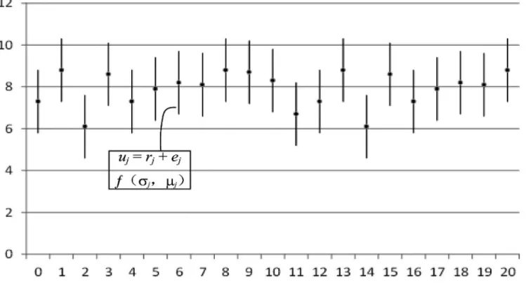
Here we have vi = (ti, ui, pj), in which ti denotes the ith sampling time point, ui denotes the ob-servation value at ti, and pi represents the prob-ability density at ti with the form of f(μj, σj) [1]. Then we have uj = rj + ej, where rj is the real value and ej is the error value.
Figure 1 shows a continuous uncertain time se-ries. The value of each time point is a random variable subject to a certain probability distri-bution with a mean of μj and variance of σj. The error function may be an arbitrary probability distribution.
Definition 3 (Uncertain time series distance).
Given two uncertain time series T1 and T2, the distance between T1 and T2 is represented by dist(T1, T2), which returns a non-negative value, indicating the distance between T1 and T2 [18]. dist(T1, T2) = (E(T1) E(T2))2 + Var(T1) + Var(T2)
It can be intuitively observed from the above formula that the expected distance can reflect data uncertainty well. First, (E(T1) E(T2))2
can become smaller along with decreasing the distance difference. Second, Var(T1) + Var(T2) indicates that the distance between two time points can become larger along with
ing the errors in the uncertain time series. It is shown that the expected distance takes the mean and the variance of uncertain time series into account, which are two important parame-ters of the uncertain time series. So, it is feasi-ble to describe uncertain time series data with the expectation and variance of uncertain data. This paper focuses on uncertain time series classification with shapelets. For this purpose, we need to evaluate subsequence quality ac-cording to the distance from subsequence to un-certain time series. In Definition 4, we present a distance definition of subsequence to uncertain time series.
Definition 4 (Distance of subsequence to un-certain time series). Let T be an uncertain time series and S be a subsequence with length l in T. Also, let Tl represent all subsequences with length l in T. Then, the distance between S and T is defined as the minimum of the distances of S to Tl and we have
subDist(S, T) = min{dist(S, Tl)}.
Definition 5 (Information gain). A shapelet is determined by a subsequence S in DB, where DB is a set of subsequences. Then the shapelet divides DB into two parts: DL and DR. The in-formation gain is calculated as follows.
( , )
| | | |
( ) ( ) ( )
| L | L | R | R
InfoGain S
D D
E DB E D E D
DB DB
Here
DL = {subdist(S, Ti) ε | Ti DB} and
DR = {subdist(S, Ti) > ε | Ti DB} We use E() to represent the information entro-py of the dataset. The definition of information gain is used to represent the quality of the time series of candidate shapelet segmentation [13]. The greater the information gain, the better the distinguishability of this shapelet. So, informa-tion gain can help to distinguish different se-quence types.
3.2. Shapelet Transformation
In this paper, we classify time series based on shapelet transformation. In this method, the
most important thing is to find the best set of shapelets, through which the raw data is mapped to new data space.
The classification algorithm based on shapelet transformation mainly consists of three steps. We first need to find all the time series subse-quences as candidates, and then evaluate all candidates and choose the best shapelet set based on the chosen assessment. Here, each shapelet represents an attribute and its attribute value is the distance between it and the time series. We finally create a new data set, which uses shapelets as feature points, and then com-plete the classification by using general classi-fication methods.
We briefly describe shapelet transformation processing in Algorithm 1. The input of this algorithm includes the pruned shapelet set and the time series set to be transformed. The out-put of this algorithm is the transformed data set. The algorithm calculates the distance of a time series to all shapelets in the shapelet collection and forms a series of new data in order (Steps 4‒7). The data is stored in the transformed data set (Step 8). The above steps are iterated until all the data in the time series set is traversed (Steps 2‒3).
Algorithm 1. Shapelet transformation.
Input:PrunedShapelet, time series set DB
Output:TD
1. TD ← ;
2. forTi in DB do //each time series in DB
3. transformed ← ;
4. forj = 0 to |PrunedShapelet| do
5. S = PrunedShapelet.get(j)
6. dist = subDist(S, Ti)
7. transformed.add(dist); 8. TD.add(transformed); 9. end for
10. end for
11. returnTD
4. PLR for Uncertain Time Series
ag-gregate approximate (PAA), piecewise linear representation (PLR), domain transformation representing, model representing, and so on. Among them, the PLR method is simple and more in line with the visual reflection of the human visual system on the sequence data. In this paper, we adopt the PLR method to per-form data dimensionality reduction of uncertain time series.
According to the partitioning strategy in the PLR, we identify two kinds of PLR. The first one is to segment the fitting error. This kind of PLR uses the straight line that connects the end-point of the segment and the starting end-point to fit the original time series. Then the least squares between the fitting curve and the original time series can be guaranteed, and the error is mini-mal. Note that this method focuses only on the local minimum error of the sequence and does not take characteristic changes in the whole se-quence into account. The second kind of PLR is the segment determined by the special points that can classify time series, say local extremum points and boundary values points. This method can avoid the global feature missing occurred in the first kind of PLR. The shortcoming of this method is that we need different methods to determine the feature points and these methods may produce large segmentation fitting errors. By default, for the uncertain time series the el-ements on all timestamps obey a certain proba-bility distribution function, where a mean val-ue is used to calculate the fitting error of each time point. Then, the linear segmentation inter-polation process can be performed. We apply a binary tree to store the key point error function. To achieve a more efficient selection process, we need a simple dimension reduction method of uncertain time series based on key points. In this way, we can improve the extraction ef-ficiency process while we maintain computa-tional accuracy to achieve stable classification accuracy. The existing dimensionality reduc-tion work on time series is mainly for certain time series.
4.1. PLR of Uncertain Time Series Based on Key Points
For an uncertain time series, we propose a sim-ple linear segmentation interpolation method
based on key points to achieve data dimension-ality reduction. In uncertain time series, the true values of all elements on timestamps are infinitely close to the mean of the probability distribution function, where the mean value is used to calculate the fitting error of each time point for linear segmentation processing.
Our method firstly finds the key points in un-certain time series according to the weight of fragments, then splits uncertain time series into several time segments with the key points, and finally completes the piecewise linear repre-sentation of the sequence. Here, all key points are put into a binary tree. Considering the un-certainty in time series and avoiding excessive noise reduction, we build a binary tree accord-ing to the index of the selected point.
In the built tree, each node stores the key point and the error function that corresponds to the key point. By obtaining key points in the binary tree, the number of segments directly achieves a fast PLR. Compared with the ordinary time series piecewise linear representation method, our method comprehensively considers the global error, segmentation error, and single in-dex point error, and to the great extent retains the global and local features of time series in the dimension reduction process. In the follow-ing, we present the definition of key points in the uncertain time series.
Definition 6 (Key point in uncertain time se-ries). In the PLR process of uncertain time se-ries, the key points must satisfy the following two conditions:
● they should be located in the uncertainty time series fragment with the largest weight, and
● the fitting error in the uncertain time series segment should be the largest.
In Definition 6, the weight of the indeterminate time series segment is related to all single point fitting errors in the segment.
1 1 1
1
( n )*(i )
i i
n
t t d
t t
The weight of an indeterminate time series seg-ment is represented as follows.
weight = max{dsum, 2 × dmax}
Here, dsum represents the sum of the fitting er-rors of the points and dmax represents the single point maximum fitting error. The maximum fit-ting error multiplied by 2 is applied in order to stress the overall error caused by a single erro-neous point.
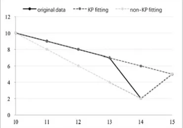
Figure 2. Example of a single point error.
Figure 2 shows the case when the overall error is small, but the single point error is large. By default, the true values of elements on all timestamps are infinitely close to the mean of the probability distribution function, where the mean value is used to represent the value at the time point. Then, the fitting error of each point is calculated and the linear segmentation pro-cessing is performed.
In Figure 2, the solid black line indicates the original sequence before segmentation. The line segmentation error threshold is set to 6, and the segmentation result is represented with the grey dotted line in Figure 2. A point with an index of 10 is considered to be a split point. Then the fit line is divided into two segments with a fitting error of 6 on the left and a fitting error of 4 on the right, respectively. Among them, the fitting error on the left is caused by 5 points, the single point error is 1 or 2, and the fitting effect is close to the original data. The fitting error on the right is only caused by a single point. The fitting error of index point 14 in Figure 2 is 4 and the fitting
effect at this time is not ideal. A simple method that is based on segmentation of the overall er-ror segmentation may result in an unsatisfactory segmentation result because such a method ne-glects the case when there is a large single point error in the segmentation.
In response to this deficiency, we apply a key point-based segmentation method. Compared to the general segmentation points, the key points contain more features of the sequence data and they can result in a good segmentation fit line. By adding a constant factor to the weight function, the observation point with a large fitting error is taken into account within the function and this can avoid the situation shown in Figure 3. The purpose why we use segmentation to represent uncertain time series is to reduce the dimension-ality of uncertain time series. For this purpose, we need to maintain the original features of data as much as possible in the dimension reduction process. As shown in the weight function defi-nition, when the weight of the segment is large, the fitting effect is poor at this time point. The reason may be that the overall error of the seg-ment is large or the single point error is large. At this time point, the time series segment with the highest weight should be continuously segment-ed. When the piecewise fitting error is less than the threshold and the single point error distance is greater than 1/2 threshold, the segmentation for the time point continues.
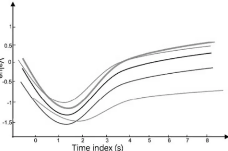
Figure 3. Time series fragment segmentation point selection.
is covered by the grey line). The light-grey dashed line represents a non-KP piece-wise fitting line, and the fitting distance of the segment is smaller than the threshold 6. Note that the single point fitting error of the index point 14 is 4, which is greater than 3. At this moment, the segmentation is performed. The final fitted line is indicated by the grey dashed line in Figure 3.
In the linear segmentation process of uncertain time series, the initial situation is that the en-tire sequence is regarded as the first segment by default. Depending on the segment weight and on whether a segmentation will continue or not, each segment for the time series segmenta-tion should preferably retain the overall or local shape characteristics of the sequence. In order to segment the time series segmentation, we need to compare the fitting distance of each time point in the segment, mark the time point with the largest single point fitting distance as the key point, and then use the key point as the dividing point to preserve the global feature of uncertain time series to the greatest extent. At the same time, for the case that the segmentation fitting error is small and the deviation of a certain time point in the segment is large, the segmentation is performed again, until the local features of un-certain time series are well reflected.
4.2. Binary Tree Construction
In order to quickly perform linear segmenta-tion of uncertain time series, the mean value of the random variable at a time point is used to represent uncertain data value. For uncertain value on the timestamp in an uncertain time se-ries, we apply a binary tree to store the error function, which corresponds to the selected key point. The choice of key points ensures that the characteristics of data fluctuations are reflected. This can avoid the missing and excessive noise removal of data feature points. As a result, we improve the extraction efficiency in the classi-fication algorithm of uncertain time series and, meanwhile, we maintain the calculation accura-cy to obtain stable classification accuraaccura-cy. For a node that is inserted into the binary tree, we have to consider the index position, the observa-tion value, the probability density funcobserva-tion, the selection order, the left and right weights of the
corresponding key points, and the left and right child nodes. Let TreeNode be an insertion node and its formal definition is given as follows.
TreeNode = {index, value, rank, f(μ, σ), weightl, weightr, childl, childr}
In the segmentation process, the key points with the largest fitting error are used for seg-mentation, and two new slice objects segment (slice.pb, slice.pmax) and segment (slice.pmax, slice.pe) are generated after segmentation. The key points and related information are stored in the binary tree. The segmenting process is iter-atively handled until there is not any segment that needs to be segmented.
By constructing a binary tree, the information of uncertain data in time series is not lost and the required key points can be obtained from the tree according to the given number of time series fragments or fragment weights. Con-structing a binary tree cannot only help the sub-sequent classification on uncertain time series but also improve the extraction efficiency by maintaining the calculation accuracy and ob-taining stable classification accuracy. The clas-sification algorithm has an advantage of being explanatory. Note that high dimensionality of time series can lead to a high time cost in the distance calculation, which makes the efficien-cy of the entire classification process lower. Therefore, a dimensionality reduction in data can effectively alleviate this problem.
For the uncertain time series after PLR, we can use the shapelet selection algorithm and pruning strategy to obtain a small number of sets of op-timal feature subsequences of retained time se-ries. We further use the shapelet transformation algorithm to get a new data set. This new data set is small and meanwhile it retains the ability to represent data characteristics. For new data sets, we can flexibly use different classifiers to achieve uncertain time series classification.
5. Shapelet-Based Classification for
Uncertain Time Series
Second, all candidate subsequences are evalu-ated according to the information gain assess-ment in order to select the best shapelets. Let each shapelet represent an attribute and then its value is the distance between the attribute to the time series. This creates a new data set. Finally, for the new data set, the general classification methods (e.g., Naive Bayes, decision trees and SVMs) can be used for classification.
5.1. Shapelet-Based Selection Algorithm
In [16], a caching algorithm was introduced for storing k best shapelets from a dataset in a sin-gle traversal. This algorithm traverses all can-didate shapelets at a time, calculates the max-imum information gain of all sub-sequences, stores them in the shapelet set, sorts them by information entropy size, removes self-simi-lar sequences, and finally collates and extracts the first k shapelets. Obviously, the number of shapelets generated with this algorithm is very large and there must be redundancy. The situa-tion becomes worse in the context of an uncer-tain time series. So, it is necessary to optimize this algorithm and eliminate redundant shape-lets so that it can participate in the shapelet con-version classification well.
Algorithm 2. All shapelet selection.
Input:DB, min, max
Output: CandShapelet
1. CandShapelet =; 2. forTiin DB do
3. shapelets =
4. for l = min: max do
5. cand = generateCandidates(Ti, l)
6. for all subsequence S in cand do
7. ds = subDist(S, DB)
8. quality = assessCandidate(S, ds) //max information gain
9. shapelets.add(S, quality);
10. end for
11. end for
12. sortByQuality(shapelets) //sort by information gain
13. removeSelfSimilar(shapelets) //remove selt-similar subsequences
14. CandShapelet.add(shapelets) 15. end for
16. returnCandShapelet
Following the step of the algorithm developed in [16], we propose Algorithm 2 for a shape-let selection. Algorithm 2 iterates through all subsequences, calculates their distance to all uncertain time series, evaluates the maximum information gain, adds them to the candidate shapelets, and then arranges them in descend-ing order of their information gain. Finally, we can get all shapelet collections after removing self-similar shapelets in the same time series.
5.2. Shapelet Pruning Algorithm
This section describes a filtering pruning method to remove similar features. This allows feature subsequences with discriminative ad-vantages to participate in data conversion. For this purpose, we iterate through all time series, perform pruning filtering on all the generated sub-sequences, remove similar sub-sequences, and then improve the quality of elements in the shapelet.
Given two shapelets S1 and S2 as well as their corresponding distance thresholds ε1 and ε2, let S1 and S2 be in the same time series class label and subDist(S1, S2) ε1. At this point, it
can be determined that S1 and S2 are similar. Here ε1 is a distance threshold that is capable of obtaining the maximum information gain, and subDist(S1, S2) ε1 means that S1 and S2 have
similar shapes. In other words, S1 can replace S2 in most cases.
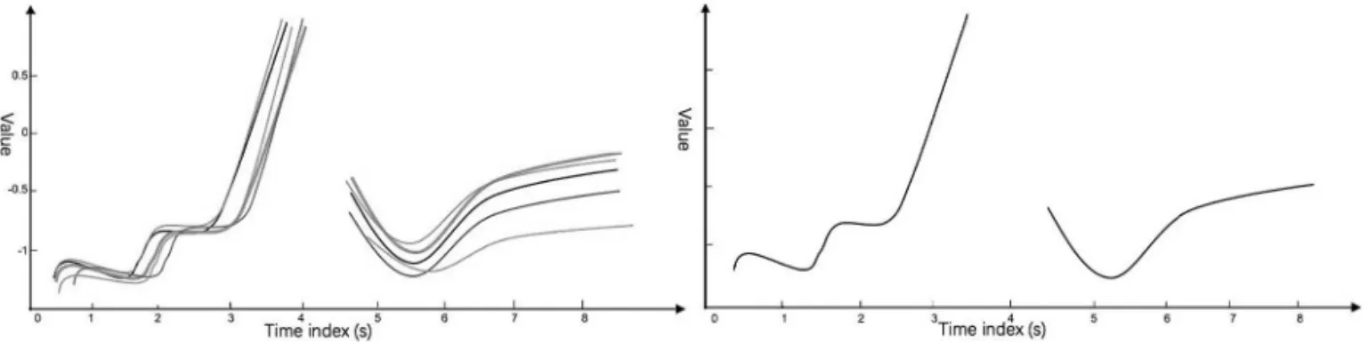
Figure 4. Five shapelets and the degree of matching when overlapping each other.
effectively reduce similar shapelets while pre-serving the shapelets that represent time series features very well.
Similar shapelets in the same time series are re-garded to be self-similarity, which is removed in Algorithm 2 (Step 13). Then, two shapelets to be compared generally exist in different time series. In this paper, we propose Algorithm 3 as our pruning algorithm.
Algorithm 3. Shapelet pruning.
Input:CandShapelet
Output:PrunedCandidate
1. PrunedCandidate ← ; 2. fori = 1:|CandShapelet| do 3. shapelet = CandShapelet[i]
4. PrunedCandidate.add(shapelet)
5. ts = shapelet.splitThreshold
6. foru = (i + 1) : |CandShapelet| do 7. prun = CandShapelet[u] 8. dist = Dist(prun, shapelet)
9. if (dist ts) //If the distance is less than ts
10. if (prun.label! = shapelet)// the class is different, keep
11. PrunedCandidate.add(prun)
12. else //If the distance is greater than the ts, keep it
13. PrunedCandidate.add(prun) 14. end for
15. end for
16. returnPrunedCandidate
For each shapelet in the candidate shapelets, Algorithm 3 compares it with the shapelet that is better than it (Steps 2‒6). When the distance between these two shapelets is less than the cor-responding threshold, Algorithm 3 compares their class labels. When their class labels are the same, we do not need to make a place in the shapelet collection (Steps 6‒11); otherwise, we put them in the PrunedShapelet (Steps 12‒13).
Finally, we get a collection of dissimilar shape-lets for shapelet transformation classification. Figure 5 shows the top ten best shapelets gener-ated for the Gun_Point dataset in [16]. It is ob-served that there are significant similarity and difference between these data (left), which can be regarded as two different types of feature subsequences. These two clusters can inter-pret the time series in an explanatory manner. Using the shapelet pruning algorithm and the expected distance for distance calculation, we remove the similar shaplelets in the same time series. We leave only a single shapelet to form a new shapelet data set (right) for subsequent data conversion and achieve a shapelet-based classification for uncertain time series.
6. Experimental Results and Analysis
In this section, we illustrate with experiments the feasibility and advantages of our approach for uncertain time series classification. First, we compare the proposed shapelet transformation classification algorithm with the algorithms pro-posed in [14], [16] and [19] in order to illustrate the usability of shapelets in classifying uncer-tain time series. Second, with different classifi-ers to classify test dataset, we illustrate that the pruning algorithm and PLR method proposed in this paper can provide better accuracy.
We used Java language to implement the algo-rithm proposed in the paper. Our experiments run in a laptop with AMD processor, Win10 op-erating system, and 8GB system memory.
6.1. Experimental Datasets
In the experiments, 17 datasets in UCR time se-ries data [20] were used as the test targets. All datasets consist of a training set and a testing set. Among them, the training set is used to per-form shapelet selection discovery and classifier construction, and the test set is used to evaluate the classification accuracy of the classifier. We artificially add interference to the UCR data to obtain uncertain data. Following the under-lying distributions of uncertain time series that are discussed in Section 3.1 (that is, a form of mean and variance), we here apply values in (0, 1) as noises, which are randomly generat-ed and may be positive or negative. The same processing is performed for all sequences. The function of arbitrary distribution with the ex-pectation of 0 and the variance of σ are used as the error function at each time point. Then the data is processed by the phased error function according to the distribution trend of the data itself, 0.1σ 2σ is used for the data of different time periods as the variance of the error func-tion. Here σ represents the standard deviation of the sample itself.
6.2. Classification Effect Comparison
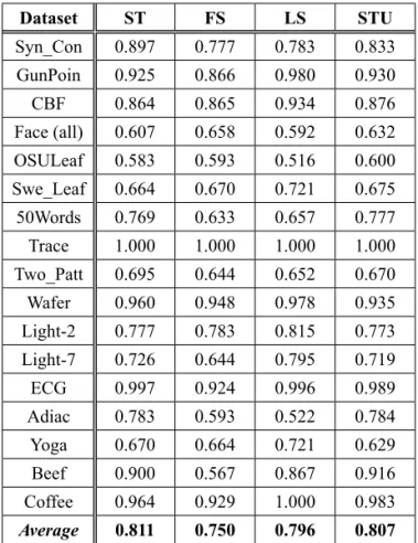
We compare our method with three shape-let-based classification methods, which are FS [14], ST [16] and LS [19], respectively. The FS represents the SAX-based fast shapelet algo-rithm proposed in [14], the ST represents the shapelet transformation algorithm proposed in [16], and the LS is the machine learning-based shapelet algorithm proposed in [19]. In this pa-per, we use decision tree classifier in the classi-fication experiments and our method is referred to as the STU. Note that, in the experiments, the methods of FS, ST and LS were proposed for certain time series and our method of STU is for uncertain time series.
We want to demonstrate that the shapelet trans-formations of uncertain time series can main-tain the similar accuracy of classification results with respect to the shapelet transformations of certain time series. For each original data-set in UCR (certain time series), say GunPoin, we respectively applied the methods of FS, ST and LS and obtained their accuracy of
classi-fication. Then, for the selected original dataset we created the corresponding uncertain dataset (uncertain time series), which was used by the STU, and obtained its classification accuracy. Table 1 presents the classification accuracy ob-tained with the above-mentioned four different methods.
Table 1. Classification accuracy with different shapelet optimization methods.
Dataset ST FS LS STU
Syn_Con 0.897 0.777 0.783 0.833
GunPoin 0.925 0.866 0.980 0.930
CBF 0.864 0.865 0.934 0.876
Face (all) 0.607 0.658 0.592 0.632
OSULeaf 0.583 0.593 0.516 0.600
Swe_Leaf 0.664 0.670 0.721 0.675
50Words 0.769 0.633 0.657 0.777
Trace 1.000 1.000 1.000 1.000
Two_Patt 0.695 0.644 0.652 0.670
Wafer 0.960 0.948 0.978 0.935
Light-2 0.777 0.783 0.815 0.773
Light-7 0.726 0.644 0.795 0.719
ECG 0.997 0.924 0.996 0.989
Adiac 0.783 0.593 0.522 0.784
Yoga 0.670 0.664 0.721 0.629
Beef 0.900 0.567 0.867 0.916
Coffee 0.964 0.929 1.000 0.983
Average 0.811 0.750 0.796 0.807
In Table 1, for a given dataset with certain numbers of classes, we extract its feature sub-sequence fragments and then calculate the dis-tances between all shapelets and the time series to be measured. The class of the shapelet with the shortest distance to the time series to be measured will be the class of the time series to be measured. Generally, we have a number of the extracted shapelets due to a dataset with nu-merous classes. The final accuracy measured is determined by the approaches for extracting the shapelets and calculating the distances.
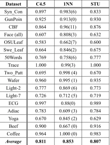
the original datasets (certain time series) in the C4.5 and 1NN and the corresponding uncer-tain datasets (unceruncer-tain time series) in the STU. Table 2 presents the classification accuracy obtained with the methods of C4.5, 1NN and STU. Note that the C4.5 and the ST are identi-cal for time series classification and, as a result, they have the same classification accuracy on the same datasets.
Table 2. Classification accuracy with different classifiers.
Dataset C4.5 1NN STU
Syn_Con 0.897 0.983(6) 0.833
GunPoin 0.925 0.913(0) 0.930
CBF 0.864 0.96(11) 0.876
Face (all) 0.607 0.808(3) 0.632
OSULeaf 0.583 0.662(7) 0.600
Swe_Leaf 0.664 0.846(2) 0.675
50Words 0.769 0.758(6) 0.777
Trace 1.000 0.99(3) 1.000
Two_Patt 0.695 0.998 (4) 0.670
Wafer 0.960 0.995 (1) 0.935
Light-2 0.777 0.869 (6) 0.773
Light-7 0.726 0.712 (5) 0.719
ECG 0.997 0.88(0) 0.989
Adiac 0.783 0.609 (3) 0.784
Yoga 0.670 0.845 (2) 0.629
Beef 0.900 0.667 (0) 0.916
Coffee 0.964 1.000 (0) 0.983
Average 0.811 0.853 0.807
Note that the ST method in Table 1 and the C4.5 method in Table 2 are identical because they apply the same method in [16]. Therefore, the shapelet optimization method ST produces the same exact results in Table 1 as the classi-fier C4.5. in Table 2. It is shown in Table 1 and Table 2 that our method can provide the similar classification accuracy with other five methods. For the given 17 datasets, totally speaking, the STU method provides a better classification ac-curacy than the methods of ST, C4.5 and 1NN, and almost the same classification accuracy as the LS method. Note that the classification ac-curacy provided by the STU method is not bet-ter than the classification accuracy provided by the FS method. But the STU method can deal
with the classification of uncertain time series and other five methods can classify only certain time series.
6.3. Algorithm Efficiency Analysis
As we know, the number of time series is usu-ally very large and the training process has high time complexity. Many efforts have been de-voted to reducing the complexity of the training process [13], [10], [15]. Suppose that the num-ber of time series objects in the dataset is k and the average length of each time series is m. In [13], Ye and Keogh used SDEA (Subsequence Distance Early Abandon) and AEP (Admissi-ble Entropy Pruning) to reduce running time and their method has the time complexity of O(m4k2). Mueen et al. in [10] tried to reduce this
complexity by caching distance calculations for future use. They introduced a pruning strategy and achieved an order of magnitude faster than the method in [13]. In [15], Hill et al. used hier-archical clustering to obtain different shapelets. The worst-case time complexity of hierarchi-cal clustering is O(k3) and after optimization,
the complexity of hierarchical clustering is still O(k2logk). The 1-NN classifier focuses on
classifying time series with optimal accuracy, which provides the best classification accuracy. However, the use of DTW-based 1-NN classifi-ers is less suitable for time series classification because it has the O(k4m4) complexity of each
instance in the training set.
The time complexity of the shapelet filter-ing prunfilter-ing method proposed in this paper is O(k2m2). It is shown that the shapelet
7. Conclusion
This paper presents a transformation for un-certain time series classification. We provide a new algorithm that just scans the datasets once and uses the pruning strategy to remove similar shapelets. Experimental results show that the proposed classifier can perform uncertain time series classification better on most datasets compared with the other classifiers. Compared with other algorithms, the algorithm proposed in the paper can provide similar accuracy and less time complexity. More importantly, the proposed algorithm can provide good interpret-ability in uncertain time series classification. Although the dimensionality reduction process can reduce the partial complexity, our method still inevitably produces some errors. Based on the characteristics of uncertainty in time series data, one of the directions for our future work is to achieve better shapelet extraction.
References
[1] L. L. Zuo and L. Yan, "A Weighted DTW Ap-proach for Similarity Matching over Uncertain Time Series", Journal of Computing and Infor-mation Technology, vol. 26, no. 3, pp. 179‒190, 2018.
https://dx.doi.org/10.20532/cit.2018.1004217 [2] R. Z. Ma et al., "A Data-Driven Analysis of
In-terplanetary Coronal Mass Eject and Magnetic Flux Ropes", in Proceedings of the 2016 IEEE International Conference on Big Data, 2016, pp. 3177‒3186.
http://dx.doi.org/10.1109/BigData.2016.7840973 [3] R. Z. Ma and R. A. Angryk, "Distance and Densi-ty Clustering for Time Series Data", in Proceed-ings of the 2017 IEEE International Conference on Data Mining Workshops, 2017, pp. 25‒32. http://dx.doi.org/10.1109/ICDMW.2017.11 [4] J. Lines et al., "Time Series Classification with
HIVE-COTE: The Hierarchical Vote Collec-tive of Transformation-Based Ensembles", ACM Transactions on Knowledge Discovery from Data, vol. 12, no. 5, p. 52, 2018.
http://dx.doi.org/10.1145/3182382
[5] T. Kieu et al., "Outlier Detection for Multidi-mensional Time Series Using Deep Neural Net-works", in Proceedings of the 19th IEEE Interna-tional Conference on Mobile Data Management, 2018, pp. 125‒134.
http://dx.doi.org/10.1109/MDM.2018.00029
[6] J. Aßfalg et al., "Probabilistic Similarity Search for Uncertain Time Series", in Proceedings of the 2009 International Conference on Scientific and Statistical Database Management, 2009, pp. 435‒443.
https://doi.org/10.1007/978-3-642-02279-1_31 [7] O. Patri et al., "Discovering Malware with Time
Series Shapelets", in Proceedings of the 50th Ha-waii International Conference on System Scienc-es, 2017, pp. 1‒10.
http://dx.doi.org/10.24251/HICSS.2017.734 [8] A. McGovern et al., "Identifying Predictive
Multi-Dimensional Time Series Motifs: an Ap-plication to Severe Weather Prediction", Data Mining and Knowledge Discovery, vol. 22, pp. 232‒258, 2011.
https://doi.org/10.1007/s10618-010-0193-7 [9] J. Lines et al., "Classification of Household
Devices by Electricity Usage Profiles", in Pro-ceedings of the 2011 International Conference on Intelligent Data Engineering and Automated Learning, 2011, pp. 403‒412.
https://doi.org/10.1007/978-3-642-23878-9_48 [10] A. Mueen et al., "Logical-Shapelets: an
Expres-sive Primitive for Time Series Classification", in
Proceedings of the 17th ACM SIGKDD Interna-tional Conference on Knowledge Discovery and Data Mining, 2011, pp. 1154‒1162.
http://dx.doi.org/10.1145/2020408.2020587M [11] A. Bagnall et al., "The Great Time Series
Clas-sification Bake off: A Review and Experimental Evaluation of Recent Algorithmic Advances",
Data Mining and Knowledge Discovery, vol. 31, no. 3, pp. 606‒660, 2017.
http://dx.doi.org/10.1007/s10618-016-0483-9 [12] L. Ye and E. J. Keogh, "Time Series Shapelets:
A Novel Technique that Allows Accurate, Inter-pretable and Fast Classification", Data Mining and Knowledge Discovery, vol. 22, pp. 149‒182, 2011.
http://dx.doi.org/10.1007/s10618-010-0179-5 [13] L. Ye and E. J. Keogh, "Time Series Shapelets: A
New Primitive for Data Mining", in Proceedings of the 15th ACM SIGKDD International Confer-ence on Knowledge Discovery and Data Mining, 2009, pp. 947‒956.
http://dx.doi.org/10.1145/1557019.1557122 [14] E. J. Keogh and T. Rakthanmanon, "Fast
Shape-lets: A Scalable Algorithm for Discovering Time Series Shapelets", in Proceedings of the 2013 SIAM International Conference on Data Mining, 2013, pp. 668‒676.
http://dx.doi.org/10.1137/1.9781611972832.74 [15] J. Hills et al., "Classification of Time Series
by Shapelet Transformation", Data Mining and Knowledge Discovery, vol. 28, no. 4, pp. 851‒881, 2014.
[16] J. Lines et al., "A Shapelet Transform for Time Series Classification", in Proceedings of the 18th ACM SIGKDD International Conference on Knowledge Discovery and Data Mining, 2012, pp. 289‒297.
http://dx.doi.org/10.1145/2339530.2339579 [17] C. Ji et al., "A Piecewise Linear Representation
Method Based on Importance Data Points for Time Series Data", in Proceedings of the 20th IEEE International Conference on Computer Supported Cooperative Work in Design, 2016, pp. 111‒116.
http://dx.doi.org/10.1109/CSCWD.2016.7565973 [18] W. K. Ngai et al., "Efficient Clustering of Un-certain Data", in Proceedings of the 16th Inter-national Conference on Data Mining, 2006, pp. 436‒445.
http://dx.doi.org/10.1109/ICDM.2006.63
[19] J. Grabocka et al., "Learning Time-Series Shape-lets", in Proceedings of the 2014 ACM SIGKDD International Conference on Knowledge Discov-ery and Data Mining, 2014, pp. 392‒401. http://dx.doi.org/10.1145/2623330.2623613 [20] Y. Chen et al., "The UCR Time Series
Classifica-tion Archive", 2015.
www.cs.ucr.edu/~eamonn/time_series_data/
Received: February 2019 Revised: November 2019 Accepted: November 2019
Contact addresses: Ruizhe Ma Georgia State University
Atlanta USA e-mail: [email protected]
Liangli Zuo Nanjing University of Aeronautics and Astronautics Nanjing China e-mail: [email protected]
Li Yan* Nanjing University of Aeronautics and Astronautics Nanjing China e-mail: [email protected]. *Corresponding author
RUIZHE MA received her PhD degree from the Department of Computer
Science at the Georgia State University, USA. Her research interests in-clude time series analysis, Big Data processing and data mining.
LIANGLI ZUO received her Master degree from the College of Computer
Science and Technology at the Nanjing University of Aeronautics and Astronautics, China. Her research interests include time series analysis and uncertain data management.
LI YAN is a full professor at the College of Computer Science and