Qualitative and Quantitative Optimization for Dependability
Analysis
Leila Boucerredj
University 08 mai1945, Guelma, Faculty of Science and Technology
Department of Electrotechnics and Automatics, BP.401, Guelma 24000, Algeria Laboratory of Automatic and Signals Annaba (LASA)
Laboratory of Automatics and Informatics Guelma (LAIG) E-mail: [email protected]
NasrEddine Debbache
University Badji-Mokhtar, Annaba, Algeria
Faculty of Science of the Engineer, Department of Electronics, Laboratory of Automatic and Signals Annaba (LASA) E-mail: [email protected]
Keywords: system controlled by computer, dependability, optimization qualitative and quantitative, truth table, Karnaugh table, reduced Markov graph
Received: March 31, 2017
Systems that are not dependable and insecure may be rejected by their users. For many systems controlled by computer, the most important system property is the dependability of the system. For this reason in this paper, we propose a complete approach for dependability analysis. The proposed approach is based on optimization qualitative and quantitative for dependability analysis, qualitative optimization is based on causality relations between the events deduced from Truth Table Method combined with Karnaugh Table for deriving minimal feared states, quantitative optimization is based on Reduced Markov Graph this graph is directly composed by a minimal feared state deduced from the qualitative optimization, to avoid the problem of combinatorial explosion in the number of states in the Markov graph modelling. The representation of the Markov graph will be particularly interesting to study dependability.
Povzetek: Razvita je inovativna metoda za kvalitativno in kvantitativno optimizacijo analize odvisnosti programov.
1
Introduction
The migration from analogical to digital components in the systems controlled by computer has increased the complexity of the systems. In this modern system, dependability is the most important aspect of system quality, in order to guarantee their functional behaviour[1]. Most of the critical failures are generated by the interactions between the sub-systems, implemented in different technologies, which is based on the disciplines of mechanical engineering, electrical engineering and information technology....Therefore, the dependability analysis, one of the most important problems for modern systems typically intelligent systems such as system controlled by computers, becomes extremely difficult. The systems having no simple interconnections are called complex and hybrid systems [2], [3], [4].
The dependability of a system reflects the user's degree of trust in that system. Dependability covers the related systems attributes of reliability, availability and security. These are all inter-dependent [3], [5], [6]. Undependable systems may cause information loss with a high consequent recovery cost [5]. The costs of system failure may be very high if the failure leads to economic losses or physical damage.
In the most current papers, the evaluation of dependability methods (evaluation of reliability and availability) are generally reserved for the simple systems (series and parallel systems) or for the components [1], [2], [5]. The dependability analysis is conventionally modeled and analyzed using techniques such as Fault Tree Analysis (FTA) and Reliability Block Diagrams (RBD), consider for example the method of reliability block diagram, is primarily directed towards success analysis and does not deal effectively with complex repair and maintenance strategies or general availability analysis, is in general limited to non-repairable systems. The analysis is limited to single failures and is time-consuming [7].
state-dependent behaviour of systems [7], so we can not represent reconfiguration [8], [9], [10]. Finally, it is not possible to take into account transient failures [4], [5], [6], [7].
The discrete events methods analyses (automats, Petri net) have their contribution in this field but the use of accessibility graph is quickly confronted to the problem of combinative explosion [4]. But, for the most part of system controlled by computers, their components are configured, where the interactions between the components are defined by logical or physical links which complicate the evaluation of the dependability of these kinds of systems.
System controlled by computer performance degradation is a stochastic process, Hence the need to use more appropriate methods for modelling and analysis of modern dynamic systems models such states transitions [6], [8], [9], [10], [11], [12]. These models include state graphs (e.g. Markov graphs).
Markov graph models (MGM) have been used to analyze computer networks [13], [14] and Programmable Electronic Systems (PES) used in industry to protect and control processes [14], [15].
Markov graph model represents the system in terms of the system states and transitions between the states, the representation will be particularly interesting to study dependability, the designer has the ability to view all of the operating modes (nominal and degraded) and the feared states of the system studied, and all failure rates (transitions) components, thereby improving the overall understanding of the behavior and evolution of the system in the presence of failures.
The aim of this work is to propose a dependability evaluation of system controlled by computer using a new approach based on optimization qualitative and quantitative analysis. The qualitative analysis optimization based on Truth Table method combined with Karnaugh Table used for focus the search of failure on the system study (or parts of the system) that are interesting for dependability analysis, the objective is to determine the causality events between nominal states, degraded state and feared state for deriving Minimal Feared State (MFS). Then we complement our study by a quantitative analysis optimization based on the construction of the Reduced Markov Graph (RMG), this graph is directly constructed by a set of minimal feared state deduced from the results of qualitative analysis. The advantage of Markov graphs lies in their ability to take into account the dependencies between components and the possibility to obtain various measurements from the same database modelling (Reliability, Availability, security...).
Despite their conceptual simplicity and their ability to overcome some shortcomings of the conventional methods of dependability, Markov graph is quickly confronted to the problem of combinative explosion in the number of states if the system is complex [5], [15], [16], [17], because the modelling process involves the enumeration of all possible states and all transitions between these states. To avoid the problem of combinative explosion of the number of states in the
Markov graph modelling, it is possible under certain assumptions (Markov assumption) modelling with Truth table (TT), combined with Karnaugh Table (KT), for deriving minimal feared state (qualitative optimization) and subsequently generates the Reduced Markov Graph (quantitative optimization), which greatly facilitates the modelling because it is more structured and more compact. As the information associated with changes of state is stochastic (transition rates), this approach is well suited to describe the failure.
The paper is organized as follows: Section 2 present the quantitative analysis by Markov graph model. Section 3 contains detailed description of proposed approach optimization. We use a case study to illustrate the effectiveness of our approach, the results and summary steps of our proposed approach are provided in Section 4. Section 5 concludes the paper.
2
Quantitative analysis by Markov
Graph
This method permits the calculation of reliability or availability of a repairable system or no with failure rates to the constant values [15], [16], [17]. It gives a representation of the causes of failures and their combination that lead to a feared situation.
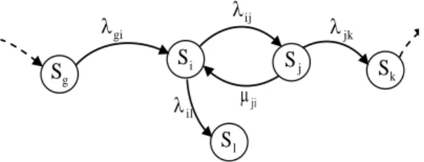
A Markov process can be represented graphically by a state-of-transition model called a Markov graph. It is an oriented graph composed by a vertices and oriented arcs (lines),
- the vertices represent the states of the process, - the oriented arcs (lines) connecting the evolution of states. This arcs are labeled by a transition rate Tij (failure rate: λ) from the state Si to the state Sj, or from the state Sj to the state Si by a transition rate Tji (repair rate: μ), so we can propose the folowing definition.
2.1
Definition (Markov Graph)
A Markov Graph (MG) is defined as a 5-tuple MG=(N, S, Tij, λ, μ) where:
- N: is a finite number of states of MG,
- S = 2N: corresponds to all possible states component of system (Sij: nominal state, feared state, degraded state...),
- Tij: continuous transition rates (failure, repair…) from Si state to Sj state.
:
,
are the backward and forward transition rates, respectively:if an arc (line) leads from the operating state i to the failure state j (
j T i S S
ij
→ ) is characterized by a constant failure rate λij [1/time unit].
if an arc (line) leads from the failure state j to the operating state i ( j
T
i
S
S
ji
) is characterized by a constant repair rate μji [1/time unit].working state to the failed state (Si to Sj). These possible transitions (
ij,
ji) are represented by the transition lines (or arc model) and arrows in the Markov Graph from one to the other states (see Figure 1):Figure 1: Markov graph representation.
The Markov Graph above (Figure 1) may be translated into a set of linear differential equations which represent the time-dependent behaviour of the state probabilities. These equations are given below.
An n state of Markov model leads to a system of n
coupled differential equations. Let P(t) be a vector that gives the probability of being in each state at time t. the system of differential equation describing the Markov model is given by:
A P(t),P(t),...,P(t)
dt ) t ( dP ., . . , dt ) t ( dP , dt ) t ( dP n 2 1 n 2
1 =
Or:
A P P= •
(2)
Where
•
P and P are n × 1 column verctors, [A] is an n×n matrix (matrix of transition rates between states) and n is the number states in the system. The solution of equation 2 is given by equation 3:
)
0
(
P
e
P
=
At
(3) WhereAt
e
is an n×n matrix and P(0)is the initial probability vector describing the initial state of the system. It can be used for system state probability evaluation at the time t (transient analysis) or in the steady state t→∞ (stationary analysis) [16].2.2
Example 1
In order to illustrate how the Markov model equations are developed, assume we have an example illustrated by figure 2
.
Figure 2: Markov Graph example.
The differential equation describing Markov Graph example (see Figure 2) is given by:
A P(t),P(t),P(t),P(t),P(t),P(t)
dt ) t ( dP , dt ) t ( dP , dt ) t ( dP , dt ) t ( dP , dt ) t ( dP , dt ) t ( dP 6 5 4 3 2 1 6 5 4 3 2
1 =
+ − − + − + − + − = 0 0 0 0 0 0 3 ) 3 4 ( 4 0 0 0 0 2 2 0 0 0 0 1 0 ) 1 2 ( 0 2 0 0 10 5 ) 10 5 ( 0 0 0 0 3 1 ) 3 1 ( A = − − − − − 0 0 0 0 0 0 3 7 4 0 0 0 0 2 2 0 0 0 0 1 0 3 0 2 0 0 10 5 15 0 0 0 0 3 1 4
The vector that gives the probability of being in each state at time t is (see equation 5):
P• =
AP[A] is defined as the state transition matrix. The solution of equation 5 is:
)
0
(
P
e
P
=
At
If we have chosen the method of state representation of Markov processes to study the dependability of a modern complex system, it is necessary to use complex algorithms for calculate the parameters of dependability (reliability, maintainability...) [13], [16], [17].
In this paper we have choose the Markov Graph Model (MGM) to study the dependability systems.MGM represent the logical behaviour of components of the system study and should contain all possible states and transitions for the state components. In the context of dependability the representation of the Markov graph will be particularly interesting to visualize all the operating modes (nominal, degraded) and the failure state of the system and all failure and repair rates (transitions) of the components, which improves the overall understanding and evolution of the system in the presence of failures.
In the next part we have proposed an algorithm to construct Markov Graph Model (MGM).
2.3
An algorithm to construct MGM
Markov Graphs (MG) is the most frequently used type model for dependability analysis. It can be used to represent hardware, software and their combined interactions in a single model to provide various information. For example, a Markov graph can determine the probability of a system being in a particular state at a particular time and it can provide estimates for both safety and reliability [14].
2 3 5 10 4 1 3 1 2 3 S 5 S 4
S S6
1 S 2 S (5) (4) (1) ij l S i S g
S j Sk
S
gi
jk
il
The first step for building the Markov graphs is to identify the different states (working or failed) that the system can occupy (2N states). The next step is to investigate how the system moves from one state to another state, by the various transitions between the states, these transitions represent the failure and the repair rates for the various components.
For construct the Markov Graph we have proposed the following algorithm.
Initialization:
Procedure Initialization:
Decompose the system into a component Ci;
Define the number of state components of the system N; Define Markov Graph Elements (MGE) MGE=(N, Si, Tij, λ, μ);
end procedure Construction:
Procedure Construction:
for each Component Ci (i = 1 to N) do
create all states Si (2N state) of the system
(working, degraded, failed);
draw all possible transitions (T) represented by the transition lines and arrows between states;
if the state of components are reparable
develop all transition failure rate and repair rate for each components;
draw the transition lines from operating state i to failure state j witch characterized by a constant failure rate λij then
draw the transition lines from failure state j to the operating state i witch characterized by a constant repair rate μji
else
draw the transition lines from operating state i to failure state j witch characterized by a constant failure rate λij
end
end end for end procedure
The major drawback of Markov graph models is that Markov diagrams for large systems are generally exceedingly large and complicated and difficult to construct. For example, the Markov graph associated to a system with N redundant components (each with two possible states: working and failed) can contain up to 2N states. For example, if we assume a system has 11 elements, each of which has two states (good and failed), the total number of possible states becomes 2N = 211 =
2048. We can see that the Markov Graphs for large systems are generally exceedingly large and complicated and difficult to construct [5], [6].
As the size of the Markov Graph increases if the systems are complex such as intelligent systems, we need use new approach to avoid the problem of combinatorial explosion in the number of states in the Markov graph modelling [16], [17], it is possible under certain assumptions (Markov assumption) modeling with Truth table method combined with Karnaugh table, to determine the minimal cut sets (Minimal feared state)
and subsequently generates the Reduced Markov Graph
(RMG), this permits simplifying the representation of MG and reducing the combinatorial explosion of the number states of the MG if the system is complex for quantitative optimization.
The proposed approach optimization for dependability analysis is developed in the next section.
3
Proposed approach optimization
3.1
Basic notation
In this section, we start with defining some basic elements of our proposed approach for dependability analysis.
3.1.1
Feared scenarios definition
A scenario can be defined as a beginning, an end and a history which describes the evolution of a system. In dependability and security study, a feared scenario leads to a catastrophic or dangerous state called feared state. The feared scenario describes how the system leaves from a nominal behavior towards the behavior in case of failure [4].
In this work the definition of a minimal feared scenario is based on the concept of ‘Minimal Cut Sets’.
3.1.2
Minimal cut sets and minimal cut vectors
A cut set is a set of components of a system whose simultaneous failure leads into the failure of the system (if the system has been operational). A cut set is minimal, if no component can be removed from it without losing its status as a cut set [18], [19] [20]. A minimum cut sets is a section containing no other cut.
Every (minimal) cut set can be represented by a state vector. This state vector is known as (minimal) cut vector [13], [15], [18], [19] [20].
The Minimal Cut Set (MCS) size is a qualitative ranking of the causal combination, based on Boolean logic [17].
The qualitative analysis proceeds by ‘Minimal Cut Sets’ is used to optimize resources in assuring system safety.
From the results of qualitative analysis (MCS) we can calculate the occurrence probability of feared state using probability technique (F (t)) [6]:
- Mechanical and hydraulic components are characterized by a Weibull distribution,
( )
t 1 ,F
e
t
− − −
= where
is the shape parameter,
is the scale parameter and
is the location parameter.- Electronic and sensor components are defined by an Exponential distribution, F
( )
t =1−e
−t,where
is the failure rate.- Software components can be characterized by,
( )
t 1 ,F
e
t + −
− =
3.2
Truth Table method and Minimal
Feared State
Based on the Boolean algebra, the Truth Table (TT) method allows identifying all the states (operations and failures) of the system based on binary behaviors [21]. The principle of this method consists of decomposing the system and identifying the failure modes of the different components, each component is characterized by an operating state (1) or by a failure state (0). It is a good tool to help understand the system functioning process and we can pick out the minimal feared scenario and expression for system reliability.
Establishing the TT of a system consists of analyzing the effects of all the vectors of the states components and determining all the malfunctions of the system. From this table, it is easy to deduce the failure combinations and failures leading to an undesirable event [21], [22], [23]. This optimizes system efficiency by minimizing the number of operations that must be performed to accomplish a given task.
Truth table is a picture of boxes 2N, where N is the number of state components system. Each box represents a combination of state components of the system. From truth table we built the output function system state. It is possible to convert Truth table to the Karnaugh table which can also be directly translated into a Boolean function [24], helps us simplify Boolean expressions of system reliability, and to obtain the minimal feared scenarios (minimal cut sets) for constructing the reduced Markov graph, this allows to optimize the quantitative analysis and to optimize dependability system.
3.3
Karnaugh Table
Karnaugh Table (KT) is a Truth table graph, which aids for simplifying the output expressions of TT into a minimal number of literals form (Minimal Cut Sets).
– Karnaugh Tables are really only good for manual simplification of expressions.
– Compared to the algebraic method, the KT process is a more orderly process requiring fewer steps and always producing a minimum expression (Minimal Cut Sets).
– KT can take on values 1 or 0, in the context of dependability 1 represents the good states of system functioning and 0 represent the failure states. Therefore can be exploited to help simplification of expressions by grouping together adjacent cases containing ones, thus aids for generate the minimum number of feared states (Minimal Cut Sets (MCS) or Minimal Feared Scenario (MFS)) in the TT which will make the system to fail if their failure occurs. To illustrate the use of TT combined with KT to find the MFS we take the following example.
3.4
Example 2 to convert TT into KT for
deriving MFS
In Truth table (TT) or Karnaugh Table (KT) anytime you have N components; you will have 2N possible combinations and 2N cases.
Consider a system having 4 components (a, b, c and d), at least two must work for the system to work.
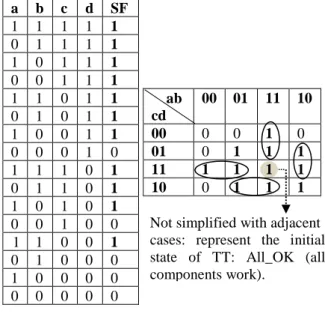
If we list all combinations (2N=4 = 16 combinations) of operational and failure states (in TT (Table 1.a) or KT (Table 1.b), (1) represents the operational state and (0) represents the failure state), we would have a table as illustrated in Table 1. The cases ‘’SF’’ represent the State Functioning (SF) of the system.
Truth table of system example is shown first (Table 1.a), the converted TT into KT is shown behind (Table 1.b).
Table 1.a: Truth Table. Table 1.b: Karnaugh Table. Table 1. Deriving MFS using TT and KT. Karnaugh table representation (table 1.b) is equivalent to the Truth table (Table 1.a), that is to say that a line of TT corresponds to a square in the KT (see Table 1).
In system example (Table 1), we illustrate the use of KT (Table 1.b) for deriving the simplified output expression associate to the TT (Table 1.a). The principle of our proposed approach for deriving MFS from TT combined with KT; the case contains “All components work”, not simplified with adjacent cases.
On inspecting Table 1 (a, b), the simplified expression (reduced to fewer terms) deduced from TT combined with KT (by grouping together adjacent cases
containing ones), for system example is given by the following expression (see equation 7):
abcd d bc c b a cd a d c b a d c b a c ab
MFS= + + + + + +
Equation 7 represents the minimal cut sets or minimal feared scenario of system example.
If it is necessary to calculate the reliability system using MFS, we can use the probability technique form [6], for calculate the reliability system from its original form components, as shown in section 3.1.2.
So from the minimal feared scenario (equation 7), we can write down the expression of system reliability (equation 8) using probability of etch state of components:
(7) a b c d SF
1 1 1 1 1 0 1 1 1 1 1 0 1 1 1 0 0 1 1 1 1 1 0 1 1 0 1 0 1 1 1 0 0 1 1 0 0 0 1 0 1 1 1 0 1 0 1 1 0 1 1 0 1 0 1 0 0 1 0 0 1 1 0 0 1 0 1 0 0 0 1 0 0 0 0 0 0 0 0 0
Not simplified with adjacent cases: represent the initial state of TT: All_OK (all components work).
ab cd
00 01 11 10
00 0 0 1 0
01 0 1 1 1
11 1 1 1 1
abc
c
b
a
c
ab
bc
a
MFS
=
+
+
+
ab c
00 01 11 10
0 0 1 1 0
1 0 1 1 1
Represent the initial state of TT: All_OK Not simplified. All components are failed
( ) ( ) ( )
( ) ( ) ( )
( ) ( )
1
P
1
P
P
P
P
( )
1
P
P
P
P
P
.
P
P
P
1
P
1
P
P
1
P
P
P
1
P
P
1
P
1
P
P
R
d c b a d c b c b a
d c a d c b a d c b a c b a
+
−
+
−
−
+
−
+
−
−
+
−
−
+
−
=
The corresponding expression for calculate the occurrence probability of feared scenario (unreliability system F (t)) from equation 8, is given by equation 9:
( )
t
1
R
( )
t
F
=
−
(9)In order to illustrate the use of TT combined with KT for construct Reduced Markov Graph (RMG) based on MFS let us consider a very simple example in the next section.
3.5
Construction of reduced Markov
Graph
In this part of paper we explain the construction of RMG using TT method combined with KT.
3.5.1
Objectives
The objective of the qualitative optimization described previously is to point out the minimal feared states based on the causal events of TT combined with KT, for analyze with precisely the causal events what makes the system leave the normal behavior and goes to the feared state; starting from the initial states ‘’all components work (all_OK)’’ in TT (to begin the analyze) that contain the necessary information to make the qualitative analysis.
The main problem encountered when analyzing critical scenarios by exploring the all states (2N) in the TT if the system is complex, anytime if you have N components, you will have 2N possible combinations, and 2N cases. In order to avoid the explosion combinatorial of states in TT we focus the search of the feared state on the part of the system that are interesting for dependability analysis, precisely is to make the Truth Table of the part of the system that leads to the feared state by exploring the all states that have a causal relation with the occurrence of the feared state, then we convert the TT to the KT for deriving MFS and then construct the Reduced Markov Graph (RMG).
The concept of the proposed approach it will: Focus the search of feared state on the parts of the system (if the system is complex) that are interesting for dependability analysis,
Define the TT of the parts (or define the TT of the complete system if the system is not complex) of the system functioning that are interesting for dependability analysis, and establish the correspondence logical expressions of each state function,
Convert TT to the KT, and the case contain “All state working” in KT not simplified with adjacent cases containing ones, for deriving MFS.
The following example should clarify the proposed approach.
3.5.2
Illustration example 3
Suppose we have a system having 3 components a, b, c (n = 3) with two components to work for the system to work. The structure function of the system example 3 is defined in Table 2. Witch “1” represents operational state and “0” failure state.
Table 2: Truth Table of system example 3. Table 2 represent the TT of system example 3, the system have 3 components, each of which have two states (good and failed); the total number of possible list of combinations states becomes 23 = 8. This all states are
presented in the TT illustrate by table 2, from this table a direct Markov Graph of system example 3 is represent in figure 3, corresponding at to all lists of combinations of operational and failure state of components ((Ci=3)=23 =8).
Figure 3: Converted TT to the Markov Graph.
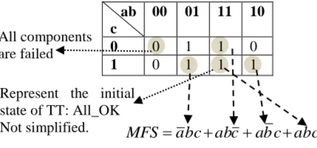
MG of the system example 3 can be reduced using the MFS deduced from the KT as shown in Table 3.
Table 3: MFS of system example 3 using KT. So for deriving Minimal Feared Scenario (MFS) using the KT (Table 3), the case represents all
list of combinations (operational and failure)
state (Ci=3) = 23 =8
State functioning (SF) of system example 3 a b c Ci
1 1 1 abc 1
0 1 1 abc 1
1 0 1 abc 1
0 0 1 abc 0
1 1 0 abc 1
0 1 0 abc 0
1 0 0 abc 0
0 0 0 abc 0
(8)
λa μa
λc μc
λb
bc a
c
b
a
c ab μb
λb
λb λc
All_OK:
abc
a
b
c
c b a μb
λa μa λc μc
λa
c
b
a
components of system example 3 works, not simplified with adjacent cases containing ones. This case represents the initial state of TT and Markov graph model.
If it is possible to generate the Minimal Feared Scenario or Minimal Cut Vector (MCV) from TT of the system study, it is not necessary to make the Table of Karnaugh. What is necessary is that the Boolean expression should be reduced to its minimal form (MFS), and then draw the Reduced Markov Graph (RMG) from MFS or MCV.
Now, as we have seen in the table 2 and 3, the system example 3 has the following MFS (equation 10):
c
ab
c
ab
c
b
a
bc
a
MFS
=
+
+
+
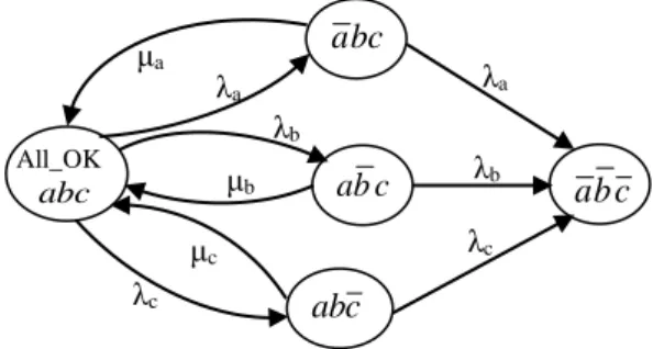
. (10) These minimal cut sets (or MFS) can be represented by the following Minimal Cut Vectors (MCV): (0,1,1), (1,0,1), (1,1,0), (1,1,1) (see Table 2 and 3).The above MG (Figure 3) can be reduced to the one show in figure 4, by using MFS or MCV as illustrated in table 2and 3, respectively.
Figure 4: Reduced Markov Graph of system example 3. In this section we see that the Markov Graph (MG) representation is very easy to construct if we use the TT method. If the system study is complex, we focus the search of feared state on the parts of the system that are interesting for dependability analysis, then create its TT combined with KT for construct the reduced Markov graph by using the concept of MFS or MCV associate to the TT combined with KT, which the case contain “All states working” in the KT not simplified with adjacent cases for deriving MFS as shown in table 3.
The Summary steps of our proposed approach are given in the next section.
4
Steps of our proposed approach
Now we need to enumerate the steps of our proposed approach of the dependability analysis as stated in section 3, the first step of our proposed approach is the: qualitative optimization.Qualitative optimization steps: this step is based on the output simplified expression (reduced to fewer terms) deduced from the causality events of TT combined with KT in order to generate automatically the MFS for construct the RMG for quantitative optimization. The summary steps of qualitative optimization are:
Step 1. Definethe number (N) of components (Ci ) of the
system study (Ci = 1 to N).
Step 2. Start to build the Truth table of the system study, If N the number of components you will have 2N possible combinations
If the system is complex,
Make the TT of the parts of the system that are
interesting for dependability analysis by identifying the all components of the part that are leads to the feared state (to guide and facilitate the search of feared state).
else
Identify all components of the system study for dependability analysis and develop the TT. Step 3. In TT begin from the initial state ‘’All_Ok’’ (correspond to all components of the system functioned correctly (if the system is complex: all components of the part of the system functioned correctly), then point out all possible combinations state of components (each components has two states ‘’working’’ or ‘’failed’’ therefore 2N possible combinations). In the context of dependability put (1) for the good state (working state) and (0) for failure state andgenerate the state function of the system study.
Step 4. Convert TT to the KT and place 1s and 0s in the squares according to the Truth table.
Step 5. In KT circle groups of casesadjacent that contain 1, but the case represents the initial state All_Ok (all components of the system in good state), not simplified
with adjacent cases containing ones. Groups may be in sizes that are power of 2: 20= 1, 21=2, 22=4, 23=8... 2N. Step 6. From KT write the simplified output expression, by grouping together adjacent cases containing ones.
The simplified output expression (reduced to fewer terms) represents the minimal cut sets or minimal feared scenario, this allows for modeling complex systems and to find the dependencies between failures, which are difficult to obtain with conventional dependability methods [10], [25].
Step 7. From the minimal feared scenario we construct the reduced Markov graph (RMG) for quantitative optimization. If it is possible to find the simplified output Boolean expression of the system study, from TT to its minimal form (minimal cut sets), it is not necessary to make the KT, then write the minimal feared scenario (MFS) or minimal cut vector (MCV) associate to the TT, and then construct directly the RMG to study the quantitative dependability optimisation.
Also from the simplified output expression, we can calculate the reliability system using probability propagation techniques [6] as shown in section 3.1.2.
Quantitative Optimization steps: from the results of qualitative optimization (MFS), reduced Markov graph are modelled (quantitative optimisation) based on minimal feared states, the states of RMG represented by circles connected by lines and arrows indicating possible transitions between the states. The transitions are conditioned, as appropriate, by process failure or repair entities down the intensity (failure rate or repair rate). This allows the representation of state dependent behaviour, including different information of components of the system and permits to obtain various λa
μa
λc μc
λb bc a
c b
a
a
b
c
c ab μb
λa λb
All_OK
abc
EV1 EV2 EV3 CP State Functioning (SF)
1 1 1 1 1
0 1 1 1 1
1 0 1 1 1
0 0 1 1 1
1 1 0 1 1
0 1 0 1 1
1 0 0 1 1
0 0 0 1 0
1 1 1 0 0
0 1 1 0 0
1 0 1 0 0
0 0 1 0 0
1 1 0 0 0
0 1 0 0 0
1 0 0 0 0
0 0 0 0 0
Table 4: Truth table of case study. measurements from the same database modelling
(Reliability, Probability of feared scenario, security...). A case study in the next section is presented to illustrate the proposed approach.
4.1
Case study
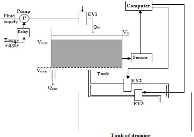
In recent years, dependability and security is an important design priority in the development and advancement of modern technology and civilization. Figure 5 show the modern automatic control system case study used for controlling and maintaining a fluid at a desired level [Vmin Vmax] in a tank controlled by computer it is composed:
- Of a pump,
-Tree electrovalve EV1, EV2 and EV3, these electrovalves have only two operating positions fully open or fully closed.
-A tank controlled (according to order of the user Qout). -A tank of draining.
-A sensor of level which provides an analogical measurement of the level of fluid in the tank.
-A computer (CP) which decides, according to the value of the volume delivered by the sensor to supply (or not) the tank by feeding (or not) the electrovalve EV1. The role of the computer is to simulate the volume (V) in the tank in real time, and giving the order of opening or closing to the tree electrovalves (EV1, EV2, and EV3). The program that automatically the computer commands the tree electrovalves (EV1, EV2 and EV3) is:
if V
Vmin open EV1 if V
Vmax close EV1If EV1 blocked open and V > Vmax
open EV2
if EV2 blocked close open EV3
end end end end
This system must avoid the overflow of the controlled tank. According to the received information from the sensor, if the volume in the controlled tank over crosses Vmax (V > Vmax) the computer actuates the electrovalves EV2 or EV3 of the system for draining the controlled tank; if the sensor identify that the volume in the controlled tank oversteps the upper limit Vmaxand if the EV2 (blocked close) is out of service (EV2_HS), the EV3 it can be used to drain the controlled tank in the tank of draining. If EV2_HS and EV3_HS, we consider the overflow of the controlled tank.
In this work we consider that only the electrovalves EV1, EV2, EV3 and computer (CP) can have failures (EV1_HS, EV2_HS, EV3_HS and CP_F (computer failed)) in the case of filing the controlled tank.
Figure 5: Case study.
4.2
Application of the proposed approach
By applying the method described in section 4, the first step is the qualitative analysis optimization for deriving MFS in order to identify the causal events leading to the overflow of the controlled tank.
4.2.1
Qualitative analysis optimization
The qualitative optimization is based on the simplified output expression (minimal cut sets) obtained from the Boolean reduction of TT method combined with KT as previously described in section 4. Our goal is to search the combinations of component failures causing system failure (overflow of the controlled thank).
For constructing the TT of case study we star with the state of all components (All_OK) in the good condition (EV1 EV2 EV3 CP) = (1111). Then we list all combinations of operational and failure state of tree electrovalves and computer (2N=4 = 16 combinations), so we have the following table (Table 4).
In this work the aim of the qualitative optimization is to determine the minimal cut sets (Minimal Feared State), by using the KT for generate the minimal number of feared state from TT. This is an efficient method to compute the Minimal Feared State of the system study based on the causality events of TT. So from the TT (Table 4) we construct the KT as shown in table 5.
Table 5: Karnaugh table of the case study.
From Karnaugh Table (see Table 5) we deduce the minimized Boolean expression form (see equation 11):
. OK _ CP OK _ 3 EV HS _ 2 EV HS _ 1 EV
OK _ CP OK _ 2 EV HS _ 1 EV
OK _ CP HS _ 2 EV OK _ 1 EV
OK _ CP HS _ 3 EV OK _ 1 EV
OK _ CP HS _ 3 EV OK _ 2 EV HS _ 1 EV
OK _ CP OK _ 3 EV OK _ 2 EV OK _ 1 EV MFS
+ + +
+ + =
The minimal feared scenario (equation 11) deduced from KT is used not only in the qualitative optimization but in all the quantitative evaluations as well. The description of a scenario as given previously (in section 3.5) can be represented by Markov Graph, this allow drawing the reduced Markov Graph for quantitative optimization studied in the next section where the cercal are the events and the lines are the transition.
4.2.2
Quantitative analysis optimization
To study the dependability of the system controlled by computer (case study), it is important, first, to model it. Therefore, the first part of the methodology that we have proposed is the qualitative analysis optimization which will provide us with all the necessary information about the operation and the dysfunction of the system study and the causal events leading to the feared state.
Quantitative evaluations are most easily performed if the minimal feared state is obtained. The aim of this section is to complement our qualitative study by the quantitative analysis based on the construction of Markov Graph, which allows a limitation of the combinatorial explosion [13], [14], [16], [17]. This graph is directly constructed from the minimal feared states (Reduced Markov Graph) obtained from qualitative
optimization. It is composed by a set of functional modes and a set of transitions to which statistical information regarding the system dynamics has been added.
This method permits the calculation of reliability or availability of a repairable system or no with failure rates to the constant values. It gives a representation of the causes of failures and their combinations that lead to the feared situation (overflow of the controlled tank), using us here the Software Reliability Workbench [26] for modelling the case study and for studies the quantitative optimization.
Reliability Workbench is Isographs flagship suite of reliability, safety and maintainability software.
So put the tree electrovalves and computer having a repair rates μ= 0.2 h-1 and a failure rates are respectively: λ= 0.02 h-1 for the tree electrovalves EV1, EV2 and EV3; and λ=0.05 h-1 for the computer (CP).
Consequently from the results of qualitative analysis (equation 11), by using the causality events of TT and KT, we directly built the Reduced Markov Graph (RMG) represented in software Reliability Workbench for quantitative analysis as shown in figure 6.
Figure 6: Reduced Markov Graph of case study.
The tops correspond to the states of the system. The lines describe the transitions between these states and a rate of transitions whose value is a constant theirs is associated. The Reduced Markov graph represented in figure (6) shows the event combinations leading to the feared states (Overflow). This graph includes the minimal failure sequences leading to the feared events.
The state All OK: all electro-valve and computer are in the good condition.
The EV1_HS state: represents the failure of EV1 (EV1_HS) and EV2 and CP in good condition.
The EV2_HS state: represents the failure of EV2 (EV2_HS) and EV1, CP in good condition.
The EV3_HS state: represents the failure of EV3 (EV3_HS) and EV1, CP in good condition.
The state "EV1, EV2 HS": represents the failure of EV1 and EV2, and EV3, CP in good condition.
The state "EV1 and EV3 HS" represents the failure of EV1 and EV3, and EV2, CP in good condition.
The state "CP_F" represents the failure of computer. The state Overflow corresponds to the failures of EV1, EV2, EV3 and CP ((EV1, EV2, EV3, CP) = (0000)), this sequence represents the overflow of the controlled tank (system state = 0).
This case represents the initial state All_OK: (EV1_OK, EV2_OK, EV3_OK and CP_OK) not simplified with adjacent cases.
This case represents the failure state of EV1, EV2, EV3 and CP (EV1_HS, EV2_HS, EV3_HS and CP_F).
EV3 CP 00 01 11 10
00 0 0 0 0
01 0 1 1 1
11 1 1 1 1
10 0 0 0 0
EV1 EV2
We have now defined the Reduced Markov Graph and can now proceed to perform an analysis.
A direct simulation in software Reliability Workbench, with 100 points and a lifetime of 450h, we obtain the following results:
Figure 7 shows the reliability of the controlled tank.
Figure 7: Reliability of the controlled tank.
A simulation shows that at time 200h the reliability of the controlled tank is: 0.11; at time 100h the reliability equal 0.33 and at time 50h the reliability equal 0.57. We can see that the reliability of the system depend on the failure states of components; it decreases rapidly as the number of failure components increases.
Figure 8, shows the Failure Frequency (FF) of overflow of the controlled tank.
Figure 8: Failure frequency of the controlled tank. Simulations show that at time 200h, FF of the system is: 0.0012; at time 100h the FF equal 0.0036; and at time 50h the FF equal 0.0062.
Figure 9 shows the evolution of Conditional Failure Intensity (CFI).
Figure 9: Conditional Failure intensity of the case study.
From figure 9, we can see that at the time instant t = 200h, 100h and 50h respectively the CFI of the system equal: 0.011.
Figure 10 shows the probability of overflow of the controlled tank.
Figure 10: Probability of overflow of the controlled tank. As Figure 10 shows, the probability of overflow of the controlled tank is: 0.89 at time 200h; 0.67 at time 100h and 0.43 at time 50h.
As confirmed by the results of the simulations we conclude that because the failure states of tree electrovalves (EV1, EV2 and EV3) and computer (CP), the probability of overflow of the controlled tank increases rapidly with time.
5
Conclusion
In this paper we have proposed a new approach for optimizing the qualitative and quantitative analysis used for dependability evaluation of modern intelligent systems such as systems controlled by computer. The first step of our proposed approach is the qualitative analysis optimization, for deriving minimal feared scenario based on causality events of Truth table combined with Karnaugh table. It is a good tool to help understand the system functioning process and we can pick out the minimal feared scenario.
Karnaugh Table process is more orderly process requiring fewer steps and always producing a minimum expression (minimal feared state) for dependability system. The combination of TT with KT presents two advantages. On the one hand, it allows a reduction of the feared state (minimal feared state), on the other hand, with the simplified output expression (reduced to fewer terms), we reduce the combinatorial explosion of the number of states of the Markov Graph (construct the RMG) for quantitative optimization. This allows for modeling complex systems, and to find the dependencies between failures. Reduced Markov graph permits the representation of state dependent behaviour, including different information of the nature of components (electronic, sensor, software,...) and system reparation. The quantitative evaluations are most easily performed if the minimal feared scenario is obtained.
The simulation with Isograph Reliability Workbench verifies the effectiveness of our approach.
6
References
[1] Elena Dubrova, Fundamentals of Dependability, Chapter 2. Book, Fault-Tolerant Design, ISBN: 978-1-4614-2112-2. ©Springer 2013.XV, 185p.
https://doi.org/10.1007/978-1-84996-414-2
[2] László Pokorádi. Failure Probability Analysis of Bridge Structure Systems. 10th Jubilee IEEE International Symposium on Applied Computational Intelligence and Informatics. Timişoara, Romania, May 21-23, 2015.
https://doi.org/10.1109/SACI.2015.7208220
[3] Albert Myers, Complex System Reliability. Springer-Verlag, London, 2010.
https://doi.org/10.1007/978-1-84996-414-2
[4] Hamid Demmou, Sarhane Khalfaoui, Edwige Guilhem, Robert Valette. Critical scenarios derivation methodology for mechatronic systems. Reliability engineering and system safety, 84 Elsevier. 33-44, 2004.
https://doi.org/10.1016/j.ress.2003.11.007
[5] CS 410/510 - Software Engineering. System Dependability. Reference: Sommerville, Software Engineering, 10 ed., Chapter 10.
[6] Fabrice Guerin, Alexis Todoskoff, Mihaela Barreau, Jean-Yves Morel, Alin Mihalache, Dumon Bernard. Reliability analysis for complex industrial real-time systems: application on an antilock brake system. IEEE International Conference on Systems, Man and Cybernetics, Hammamet, October 6-9, 2002. https://doi.org/10.1109/ICSMC.2002.1175666 [7] Cristina Johansson. On System Safety and
Reliability in Early Design Phases: Cost Fo cused Optimization Applied on Aircraft Systems. Linköping University Electronic Press, Sweden. Thesis, ISSN 0280-7971; 1600. 2013. p. 62
URN: urn:nbn:se:liu:diva-94354
[8] Pierre-Yves Piriou. Contribution to model Based Safety Analysis for dynamic repairable reconfigurable systems. Paris-Saclay University. Thesis presented at ENS Cachan, 27/11/2015. https://tel.archives-ouvertes.fr/tel-01251556
[9] Krishna B. Misra. Handbook of Performability Engineering. Book. Springer-Verlag London, 2008 https://doi.org/10.1007/978-1-84800-131-2
[10]Manno, Gabriele Antonino. Reliability modelling of complex systems: an adaptive transition system approach to match accuracy and efficiency. PhD Thesis, University of Catania, 2012.
http://archivia.unict.it/bitstream/10761/1039/1/MNN GRL82L03C351S-PhD_Thesis_GM_A.pdf
[11]Norman B. Fuqua. The applicability of Markov analysis methods to Reliability, Maintainability, and Safety. Selected Topics in Assurance Related Technologies, Vol. 10, N. 2. Reliability Analysis Center, 2003.
https://www.dsiac.org/sites/default/files/reference-documents/markov.pdf
[12]IEC 61165. Application of Markov techniques. International Electrotechnical Commission. 2006. [13]Bateman. K. A., Cortes. E. R. Availability
Modeling of FDDI Networks, Proceedings of Annual Reliability and Maintainability Symposium, IEEE. pp. 389-395, 1989.
https://doi.org/10.1109/ARMS.1989.49632
[14]Kaufman. L.M., Johnson. B.W. Embedded Digital System Reliability and Safety Analyses. NUREG/GR-0020. University of Virginia. Department of Electrical Engineering Center for Safety-Critical Systems -Thornton Hall Charlottesville, VA 22904. xi, 75 p. 2001.
[15]Paraskevas Stavrianidis. Reliability and Uncertainty Analysis of Hardware Failures of a Programmable Electronic System. Reliability Engineering and System Safety, Elsevier, vol. 39, issue 3, pp. 309-324, 1993.
https://doi.org/10.1016/0951-8320(93)90006-K [16]Raphaël Schoenig. Definition of a design
methodology for mechatronic systems including dependability analysis. PhD thesis of the National Polytechnic Institute of Lorraine, 2004.
https://tel.archives-ouvertes.fr/tel-00126057
[17]Salem Derisavi, Peter Kemper, William H. Sanders. Lumping Matrix Diagram Representations of Markov Models. International Conference on Dependable Systems and Networks. Yokohama, Japan. IEEE, pp. 742–751, 2005.
https://doi.org/10.1109/DSN.2005.59
[18]Way Kuo, Xiaoyan Zhu. Relations and generalizations of importance measures in reliability. IEEE Transactions on Reliability, Vol. 61, N. 3, pp. 659–674, 2012.
https://doi.org/10.1109/TR.2012.2208302
[19]Sally Beeson, John D. Andrews. Importance measures for noncoherent-system analysis. IEEE Transactions on Reliability, Volume 52, issue: 3, pp. 301–310, 2003.
https://doi.org/10.1109/TR.2003.816397
[20]Elena Zaitseva, Vitaly Levashenko, Jozef Kostolny, Miroslav Kvassay. Algorithms for Definition of Minimal Cut Sets in Reliability Evaluation of Green IT System. Department of Informatics, University of Zilina, Zilina, Slovakia. 2015.
https://www.pdffiller.com/jsfiller-desk5/?projectId=226202130&expId=3950&expBra nch=1#834b8f1bbf854c3e9f4c996e3b01e38a [21]Alain Villemeur. Dependability of industrial
systems. Collection of the Direction of Studies and Research of Electricity France, ISSN 0399-4198, Volume 67, 795 pages. Eyrolles, 1988.
[22]Pankaj Bansod. System Reliability and Challenges in Electronics Industry. SMTA Chapter Meeting 25th September 2013, India.
https://pdfs.semanticscholar.org/presentation/64e3/b 4774be3dad7f988fb5893a1a174e6cfabfa.pdf [23]Popov Peter, Manno Gabriele. The effect of
SAFECOMP 2011. Lecture Notes in Computer Science, vol. 6894, Springer, Berlin, Heidelberg, pp. 1-14, 2011.
https://doi.org/10.1007/978-3-642-24270-0_1 [24]Peter Cheung Professor. Lecture5: Logic
Simplification & Karnaugh Map. Department of EEE. Lecture 5 - Imperial College London. 2007. [25]Enrico Zio. Reliability engineering: Old problems
and new challenges. Reliability Engineering & System Safety, Elsevier, Vol. 94(2), pp. 125–141, 2009.
https://doi.org/10.1016/j.ress.2008.06.002 [26]