Comparison of Maximum Allowable Pump Speed in a Horizontal and Vertical Pipe of Equal Geometry at Constant Power

Comparison of Maximum Allowable Pump Speed in a Horizontal

and Vertical Pipe of Equal Geometry at Constant Power

D. Bashar1, A. Usman2, M. K. Aliyu3 and D. S. Yawas3,

1. Shell Chair Office, Department of Mechanical Engineering, Ahmadu Bello University, Zaria. 2. Department of Chemical Engineering, Ahmadu Bello University, Zaria

3. Department of Mechanical Engineering, Ahmadu Bello University, Zaria. Corresponding Author: [email protected]

Abstract

This work determines and compares the maximum possible velocity fluids can be transported through a vertical and horizontal pipe of the same geometry at constant pump power. The analysis involves simulation of theoretical piping equations, analysis of the pumping, frictional and static pressure with respect to flow velocity using MS excel and Matlab. Computational results obtained from MS excel and represented graphically in Matlab establishes the maximum allowable velocity – below which the fluid can be transported safely within the required flow input conditions (i.e. diameter, length and pump power) and above which it will be impossible for the fluid to be pumped to the given height or length under the same flow conditions. It was also found that the maximum allowable velocity is always greater in a horizontal pipe than in a vertical pipe but with pumping pressure higher in the later. In addition, a general equation was determined for approximate determination of the maximum fluid velocity given pipe length (height), pump power and pipe diameter.

Key Words

1. Introduction

Pump and piping design is very important economically (to the oil and gas industries) and politically (to the oil producing nations)as the networks of pipes in the US, Europe and Russia are respectively about 500,000km, 400,000km and 300,000km[1].Pipelines are categorized based on their usage that includes; gathering pipes- pipes with pipes large diameters at high pressure of about 4.93MPa, transportation pipelines-for transmitting product from source to supply with pressure of between 1.3-1.8MPa and distribution pipelines- conveys products to customers at pressure not greater than 1.4MPa [2].Centrifugal pumps are used for low (to moderate) pressure and high flow (high velocity) applications. The flow characteristics of a centrifugal pump changes as the pressure changes. Increasing the number of vanes of an impeller in a centrifugal pump will increase flow and reduce pressure and decreasing the number of vanes of the impeller will reduce flow and increase pressure [3].

Most industrial pumps are operated at high

horse power. Positive displacement pumps [4] classified as rotary pump typically work at pressures up to 25 bars (2.5MPa) and reciprocating pumps with pressures up to 500 bars (50MPa). Centrifugal pumps are preferred for moving large volumes of liquid at moderate pressure while positive displacement pumps are desired for moving small volume of fluids at higher line pressures [5]. Positive displacement pumps are used for products with high viscosity such as heavy crude oil, bunker fuels and asphalt while centrifugal pumps are used for light viscosity liquids such as water, gasoline, diesel oil and very light crude oil. A typical 6-stage centrifugal pump running at 3500 rpm can produce a differential pressure of up to 395psi (2.72MPa) along the pipe length [6]. Also, an industrial centrifugal pump with a capacity of 230 Hp (171.5KW) running at 2300 rpm can discharges water at a rate up to 340 m3/hr [7]. Large centrifugal pumps of over 100 Hp(73.6 KW) can be compared with positive displacement pumps for the same service [8]. The aim of this simulation is to compare maximum flow velocity in horizontal and vertical pipes of equal geometry and to optimize pump

power(for centrifugal pumps) so that fluid flow in pipes can be transported within the optimum permissible flow velocity and at a comparatively lower pump power. This will enhance energy power savings where unnecessary high horse power pumps may not be needed since comparatively lower horse power pumps can still provide the same functions the former can provide.

2. Methodology

2.1 Theoretical Background

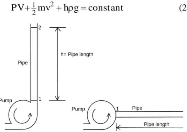
Flow at any point within a pipe is represented by the general Bernoulli’s energy equation [9] as:

t tan cons mc g h mv

PV₂1 2    (1)

Where

P = Pressure V = Volume of Flow v = Flow velocity m = Mass of fluid

c = Specific heat capacity of fluid g = Acceleration due to gravity, and

 = Temperature

Equation 1 implies that the sum of the fluid energy, kinetic, potential and internal energy is constant at any section of the pipe. This also satisfies the conservation of energy principle law. When the temperature is constant, internal energy becomes zero and equation (1) becomes:

t tan cons g h mv

PV₂1 2   (2)

2

1

h= Pipe length

Pump Pipe

Fig.1: Pumps transfering fluid to a vertical and horizontal path

Pump Pipe

Pipe length

1 2

Fig. 1 Pumps transferring fluid to a vertical and horizontal path

Bernolli’s equation for real fluid can be written as [8]; L 2 2 2 g P 1 2 1 g P h z v g 2 1 z v g 2 1 ₂

1      



 (3)

But since the pipe diameter is constant from 1-2 for the vertical pipe, v₁v₂ and equation (3) becomes: L 2 g P 1 g P h z z 2

1    

  L 1 2 g P g P h ) z z ( 2

1    

  L 1 2 2

1 P g(z z) gh

P     (4)

But





g 2 V o D fl L 2 i K

h   and pipe length

l h ) z z

( ₂ ₁   (pipe length = elevation height), we have:





P

P_{1 2 D}fl _o V₂2

i 



 (5)

In pumping fluid to a certain height (Fig.1), the total pressures needed to be overcome are the frictional pressure drop and pressure due to static height (equation 5). These are designated reaction pressure in this research work. The pumping pressure must be equal to or greater than this reaction pressure for the fluid to move to the required height and above. These can be represented in equation as;

) P P (

P_p ₁ ₂ or P_pP_f, implying the (total) pumping pressure:





P_{p D}fl _o V₂2

i      (6)

For the horizontal pipe in Fig. 1, elevation,

0 h ) z z

( ₂ ₁  

,





2.2 Obtaining Relevant Input Data

Relevant input data values obtained where tabulated appropriately in Table 1. Densities and kinematic viscosities of fluids were obtained appropriately [11]. Water is used as fluid medium in the analysis. Other fluids can also be used from the general equation determined in equation 11. Initial calculation of Reynolds number indicates that the flow is turbulent for all the velocities considered. The kinematic fluid viscosity of water is found to be 1.10e7m2/sat 20 ˚C [12].

Table 1 Input Parameters for determination of maximum velocity

Sr. No.

Data Symbol Input

Value

Comment

1.0 Flow (average) velocity (m/s)

v 2.0 Varied accordingly 2.0 Pipe length (m) _l 50 Varied

(100, 400) 3.0

Pipe diameter (mm) Di

100 Varied (40, 10) 4.0 Pump Power (KW) P 5 Constant 5.0 Pump Efficiency ç 90 Constant 6.0 Fluid Kinematic

viscosity of water at 20 ˚C (m2/s)



water at 20 ˚C (kg/m3)



coefficient-pipe i.e. piping fittings

o

K 1 Constant

9.0 Specific roughness factor (mm)



3. Relevant Assumptions

 The design is considered only for the internal flow conditions only i.e. the ideal and minimal conditions required to safely pump fluid to a certain height without abnormal and occasional influences, hence pipe thickness is not considered.

 Fluid temperature is assumed constant. Therefore internal energy and vapour pressure are

neglected. Though if present they do not impede pump pressure but ultimately add to it which relieves pump power. Their inclusion is relevant when in actual pipe design i.e., pressure integrity analysis [13] where thickness has to be compensated for the inclusion so that the pipes do not explode in operation.

 Effects of pressure transients due to sudden and gradual conditions are also neglected since they fall outside the normal or ideal requirement of lifting fluid to certain height. This happen as a result of sudden or gradual closure of valves attached to piping systems where fluid pressure subsequently increase up to the speed of sound and could have devastating consequences on piping system [14]. Occasional loads as a result of snow, earthquake, external loadings and other harsh environmental conditions are also neglected.

 Water is assumed to be the fluid medium. Flow medium is also assumed incompressible to simplify theoretical analysis [15].

 Atmosphere pressure is neglected. Mild steel is assumed to be the piping material.

4. Simulation of Theoretical Equations

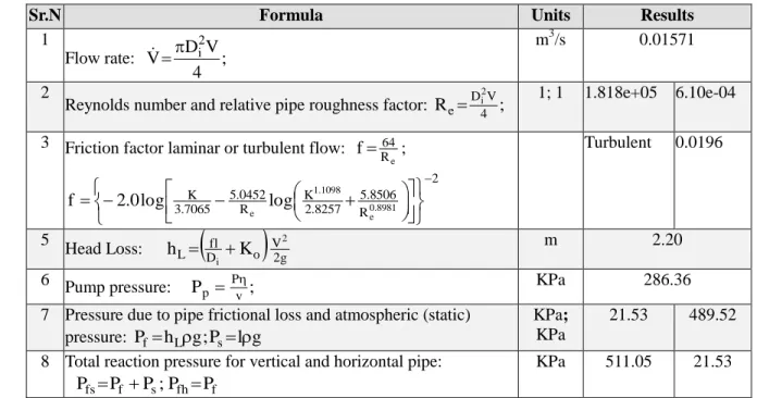
Table 2 shows the computation of flow parameters, frictional factor, pumping pressure and total reaction pressure to be overcome. Chen friction factor (more exact) approximation equation was used Table 2: Computation of result output

Sr.N Formula Units Results

1

Flow rate: ; 4 V D V 2 i    m 3

/s 0.01571

2

Reynolds number and relative pipe roughness factor: R_e D₄V;

2 i

 1; 1 1.818e+05 6.10e-04 3 Friction factor laminar or turbulent flow:

e

R 64

f ;

2 R 8506 . 5 8257 . 2 K R 0452 . 5 7065 . 3 K 8981 . 0 e 1098 . 1 e log log 0 . 2 f                  _   

Turbulent 0.0196

5

Head Loss: _L





i K

h   m 2.20

6 Pump pressure: P ;

v P p



 KPa 286.36

7 Pressure due to pipe frictional loss and atmospheric (static) pressure: P_fh_Lg;P_slg

KPa; KPa

21.53 489.52 8 Total reaction pressure for vertical and horizontal pipe:

P_fsP_f P_s;P_fhP_f

in calculation of friction factor for turbulent flow [16]. The head loss formula in Table 2 (5) is applicable for both laminar and turbulent flows [14].Table 2 depicts a single simulation result (a point coordinates in Fig. 2) for the input parameters of Table 1.

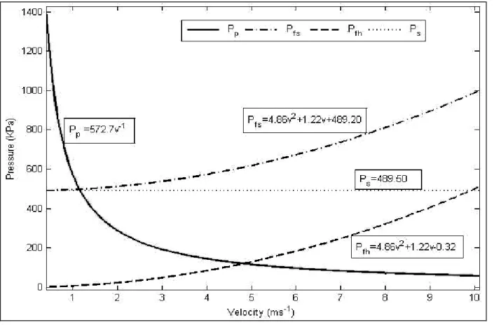
5. Result Analysis

In principle, the total pumping pressure must be greater than the total reaction pressure. The graph of the pumping pressure (representing thick line),reaction pressure for vertical pipe (representing dashed-dotted lines), reaction pressure for horizontal pipe (representing dashed lines) and static pressure (representing dotted line) are therefore plotted against varying flow velocity. From Fig. 2, it can be seen that the pumping pressure decreases and the reaction pressures (in both vertical and horizontal pipe) increases as the velocity increases until a point is reached when they are equal and above which the reaction pressure dramatically exceeds the pumping pressure. The velocity at which the pumping and reaction pressure are equal is the maximum velocity the fluid can attain at specified height given the required flow conditions. The allowable flow velocity range is when net pressure (difference between pumping and reaction pressure) is positive. For Fig. 2, the maximum possible velocities for the vertical and horizontal path are at 1.15m/s and 4.82m/s and the allowable velocity ranges are between 0 < v <1.15 and 0 < v <4.82. The frictional pressure loss (difference between the dotted and the dashed lines) is significant only within the allowable velocity range for the horizontal pipe.

Similarly, from Fig. 3, the maximum possible velocities for both pipe paths are at 3.59m/sand 5.87m/s and the allowable velocity ranges are between0 < v < 3.59 and 0 < v < 5.87. The frictional pressure losses are both significant (difference between the dotted and the dashed lines) within the allowable velocity range. Also from Fig. 4, the maximum possible velocities for both pipe path are at 0.47m/s and 2.72m/s and the allowable velocity ranges are between0 < v < 0.47 and 0 < v < 2.72 respectively. The frictional pressure loss here is only significant within the allowable velocity range for the horizontal pipe.

Frictional pressure loss for the vertical pipe of Fig. 2 and Fig. 3 can be neglected since the

dashed-dotted and the dashed-dotted lines meet the thick line at approximately the same velocity (ignoring frictional pressure means the only reaction pressure to be overcome is the static pressure which is constant). However, the frictional loss cannot be ignored for Fig. 3 and horizontal pipe path of Fig. 2 and 4 since the dashed and dotted lines meet the thick line at different maximum velocities. In other words, the maximum allowable flow velocity in Fig. 3 can only be 3.59m/s and not 4.75m/s (intersection of the dashed-dotted line with the thick line) for the vertical pipe path.

However, the effect of change in pipe length and diameter respectively is also considered. It can be noted that as the diameter (from Fig. 2 at 100mm) decreases to 50mm in Fig. 3, the pumping pressure changes (from P_p572.7v1 to P_p 2291v1 and the maximum allowable velocity increases and consequently the velocity range (as in shown in Fig. 3). It can be seen that as the length (from Fig. 2 at 50m) increases to 500m in Fig. 4, the maximum allowable velocity decreases and consequently the velocity range (as in shown in Fig. 4) but the pumping pressure is maintained (i.e. P_p 2291v1). All the three graphs are produced at constant power of 5KW. This shows that pumps can be optimized (redesigned or reengineered) at lower power to transport liquid at much longer distances.

5.1 Determination of the Maximum Fluid Velocity from Simulation

The maximum allowable flow velocity can also be calculated using equations generated for Figures 2, 3 and 4 in Matlab (curve fitting tools). The intersection of the total action and reaction pressures gives an equation in form of velocity which can be calculated as given below:

2 . 489 v 22 . 1 v 86 . 4 v 7 .

562 1 2  for the

vertical pipe path (from Fig.2)

0 2 . 489 v 22 . 1 v 86 . 4 v 7 .

562 1 2   (8)

32 . 0 v 22 . 1 v 86 . 4 v 7 .

562 1 2  for the

horizontal pipe path (from Fig.2)

0 32 . 0 v 22 . 1 v 86 . 4 v 7 .

Solving using Matlab gives three roots; one real number and 2 complex numbers. The real number is the maximum allowable velocity. The real and corresponding complex roots for the vertical and horizontal path respectively are;

, 0 ) v 15 . 1

(   implying v1.15 and

, 0 } v ) 70 . 0 i 09 . 10

{(    implying

) 70 . 0 i 09 . 10 (

v  

, 0 ) v 82 . 4

(   implying v4.82 and

, 0 } v ) 53 . 2 i 25 . 4

{(    implying

) 53 . 2 i 25 . 4 (

v  

Similarly for Figure 3, after simplifying, the real and corresponding complex roots for the vertical and horizontal path respectively are;

0 ) v 59 . 3

(   , implying v3.59 and

, 0 } v ) 93 . 1 i 44 . 7

{(    implying

) 93 . 1 i 44 . 7 (

v  

0 ) v 87 . 9

(   , implying v5.87 and

, 0 } v ) 07 . 3 i 17 . 5

{(    implying

) 07 . 3 i 17 . 5 (

v  

Similarly for Figure 4, after simplifying, the real and corresponding complex roots for the vertical and horizontal path respectively are;

0 ) v 47 . 0

(   , implying v0.47 and ,

, 0 } v ) 35 . 0 i 867 . 6

{(    implying

) 35 . 0 i 86 . 6 (

v  

0 ) v 72 . 2

(   , implying v2.72 and

, 0 } v ) 48 . 1 i 42 . 2

{(    implying

) 48 . 1 i 42 . 2 (

v  

5.2 Determination of Maximum Velocity Using Derived Equation

From equation 6, the total pumping pressure must be greater than the reaction pressure (From Table 2, Items 8 and 9) written as;

s f p fs

p P P P P

P     (10)





v A P i       simplifying;





v A

P

i     

 

simplifying;

Substituting area, D₄

2 i



 , we have





v D P 4 i 2 i       

 _{, and hence a}

general equation can hence be written as:

0 c bv2

av_{   (11)}

Where a ;b





v D P 4 i 2 i        _and g l

c  i.e., for vertical pipe and i.e. for a horizontal pipe.

The maximum velocity was determined using equation 11 for each of parameters in Fig. 2, 3 and 4 and solved graphically as depicted in Fig. 5, 6 and 7. The only constraint using the equation is determining the frictional factor, f. The friction factor was calculated from an average of two reasonably assumed velocities (1 and 4m/s). Equations from simulation (Fig. 2, 3 and 4) were plotted along side with equations generated using equation 11 as depicted in Fig. 5, 6 and 7.

Equations generated from equation 11 using same parameters as in Fig. 2, 3 and 4 for the vertical (Equation 11) and horizontal (Equation 12) path are respectively given below:

; 0 5 . 489 v 5 . 5 v 7 .

572 1 2 

; 0 5 . 489 v 4 . 10 v 9 .

2290 1 2 

; 0 2 . 4895 v 8 . 99 v 9 . 90 .

22 1 2  (12

0 v 4 . 10 v 9 . 2290 ; 0 v 5 . 5 v 7 .

572 1 2 1 2

; 0 v 8 . 99 v 9 .

2290 1 2 (13)

Analysis of the maximum velocity from equation and simulation are depicted in Table 3 below:

5.3 Graphical Determination of the Real Root and Exit Pressure Using the General Equation

Analysis of the maximum velocity determined using equation 11 and simulation (of Table 1 and 2) results were plotted in excel to determine the real roots. asically Figs. 5, 6 and 7 are graphical method (instead of using Matlab) of finding the roots of equation 11 and simulation results (Figs. 2, 3 and 4).

Table 3: Comparison of the accuracy of the maximum velocity using equation and simulation

Item

Equation: (m/s) Simulation: (m/s) Percentage Error (%)

Corrected Maximum Velocity for Equation: (m/s)

V H V H V H V H

Fig. 2 1.15 4.82 1.16 4.72 -0.87 -2.07 0.77 3.21 Fig. 3 3.59 5.87 3.65 6.04 -1.67 2.90 2.39 3.91 Fig. 4 0.47 2.72 0.47 2.84 0.00 4.40 0.31 1.81 Note: V means vertical and H horizontal

Fig. 2 Effects of pressure with velocity for a 5kw, 50m and 100 mm pump power, pipe length and pipe diameter respectively.

Fig. 3 Effects of pressure with velocity for a 5kw, 50m and 50 mm pump power, pipe length and pipe diameter respectively.

Fig. 4 Effects of pressure with velocity for a 5kw, 500m and 50 mm pump power, pipe length and pipe diameter respectively.

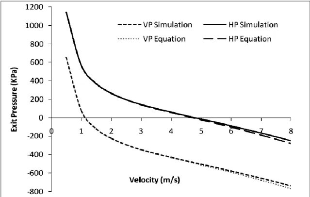
The exit pressure is the net pressure between the pump pressure and reaction pressure. This is evaluated from Table 2 as (P_pP_fs) and (P_pP_fh)

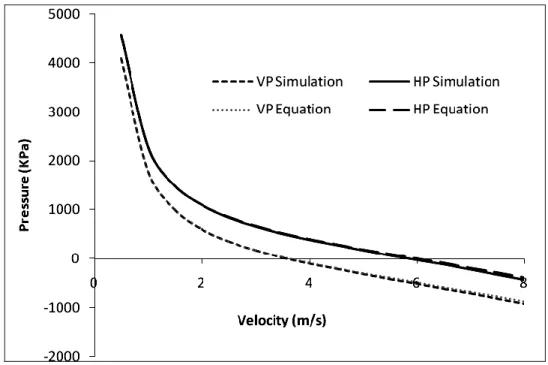
for the vertical and horizontal pipes respectively. Fig.5 depicts the variation of net exit pressure with increasing velocity for the simulation of Fig. 2 i.e. at pump power of 5KW, pipe length of 50mm and pipe diameter 100mm. As the net pressure decreases, it reaches a point when the pump pressure and the reaction pressure are equal (net pressure is zero) and the velocity at this point (1.15m/s for vertical pipe) on the graph represents the maximum allowable velocity as further decrease in the net pressure will result in an insignificant (negative) value. The graphical representation using equation 11 and simulation coincides (are equal) and with little deviation at lower negative net pressure.

Similarly, Fig. 6 depicts the variation of net exit pressure with increasing velocity for the simulation of Fig. 3 i.e. at pump power of 5KW, pipe length of 50mm and pipe diameter 50mm. As the net exit pressure decreases, it reaches a point when the pump pressure and the reaction pressure are equal (net exit

pressure is zero) and the velocity at this point (3.59m/s for vertical pipe) on the graph represents the maximum allowable velocity as further decrease in the exit pressure will result in an insignificant (negative) value.

Fig. 7 also depicts the variation of net exit pressure with increasing velocity for the simulation of Fig. 3 i.e. at pump power of 5KW, pipe length of 500mm and pipe diameter 50mm. As the net exit pressure decreases, it reaches a point when the pump pressure and the reaction pressure are equal (net exit pressure is zero) and the velocity at this point (0.47m/s for vertical pipe) on the graph represents the maximum allowable velocity as further decrease in the exit pressure will result in an insignificant (negative) value.

The allowable velocity range from Fig. 5, 6 and 7 for the vertical and horizontal pipes respectively are given as:

Fig. 5; (0 < v < 1.15);

(0 < v < 4.82)

(0 < v < 5.87)

(0 < v < 2.72)

Fig. 6 Effects of Pipe Exit Pressure with Increasing Velocity for Fig. 3.

The allowable velocity range that corresponds to the appropriate net exit pressure required can be selected and it is advisable to apply a factor of safety of two-third (2/3) to the calculated maximum velocity (for that using equation 11) since this will always fall within the actual velocity range (Table 3, columns 8 and 9).

The selected velocity (within the allowable range) can then be used to calculate the pump pressure and consequently the flow rate of the desired pump. Results of Fig. 2, 3 and 4 shows that pumps (i.e. centrifugal pumps) can be designed with high pressure and lower flow for vertical fluid path and low pressure and higher flow for a horizontal flow path.

6. Conclusions

Large centrifugal pumps of over 100 Hp (73.6 KW) are used to move fluids within long distances. Centrifugal pumps can be designed with high pressure and lower flow for vertical fluid path and low pressure and higher flow for a horizontal flow path. This can be achieved by either increasing the number of vanes of an impeller for increased flow and reduced pressure or decreasing the number of vanes of the impeller for decreased flow and increased pressure [3]. Analysis of pump pressure and parameters in this research work shows that pumps can be redesigned or re-engineered at lower power to transport liquid at much longer distances. This will enhance energy power savings where unnecessary large industrial pumps may be substituted with comparatively lower horse power pumps and still deliver fluid products effectively.

The result of the findings shows that:

 At any constant pump power and flow requirements (i.e. diameter, length and fluid medium), a maximum allowable velocity is established – below which the fluid can be transported safely to the required height or length and above which it will be impossible for the fluid to be pumped to the given height or length under the same flow conditions

 The maximum permissible velocity is always greater in a horizontal pipe than in a vertical pipe placed perpendicular to ground but a higher pumping pressure is always required in the later.

 A general equation is established that determines the maximum allowable flow velocity for pumps given the required length, diameter and pump power. The equation has three roots- a real and corresponding two equal complex roots. The real root corresponds to the maximum allowable flow velocity:

0 c bv2

v

a_{  }

Where a ;b





D P 4

i 2 i

     

 

i.e., vertical pipe and c = 0 i.e., for a horizontal pipe.

The solution of the general equation is an approximate one with a percentage error of not greater than ±4%. This is because the friction factor cannot be accurately calculated at each varying velocity. The friction factor was calculated from an average of two reasonably assumed velocities (1 and 4m/s). It will also be advisable to apply a factor of safety of 2/3 to the calculated maximum velocity since this will always fall within the actual velocity range;

d v

0 ₃2 Where d is the real root from the general equation.

 It is advisable to plot the general equation in either MS excel or Matlab in order to choose the appropriate velocity (within the allowable velocity range) that corresponds to the required net exit pipe pressure so desired.

 At constant pump power, as the diameter decreases, the maximum allowable velocity increases and as the length increases the maximum allowable velocity decreases.

Therefore the greater the pipe length and diameter, the lower the maximum allowable flow velocity for each respectively. Conversely, the lower the pipe length and diameter, the greater the maximum allowable flow velocity and its range respectively.

 Inclusion of frictional pressure drop in piping system is very significant as neglecting it sometimes may result in choosing the inappropriate flow velocity.

References

[1] Berisa M, Lesis V and Didziokas, R, Comparison of pipe internal pressure calculation methods based.MECHANIKA, 4(54): 5-12, 2005.

[2] Energy. (2012). Retrieved March 20, 2012; energy.about.com/do/drilling/a5-Types-Of-Natural-Natural-Gas-Pipelines.htm

[3] Ragsdale.Engineering and Design; New Mexico Water System O & M. Pump and Motors, Santa Fe,New Mexico 2001.

[4] HI (2013). Variable speed pumping, a guide to successful applications, www.pumps.orgaccessed 23, December, 2013. [5] P harris T. C. and Kolpa R. L. Overview of the

Design, construction and operation of interstate liquid petroleum pipelines. US department of energy, Oak Ridge, US, December, 2000. [6] Brennan J. R. Rotary pumps on pipeline

services. Tutorial presented at the Pumps Users Expo 200, Louisville, KY, September 2000. [7] Global Spec. 18” Non-Clog Pump, Griffin Pump

and Equipment Inc.,

http://www.globalspec.com/industrial-directory/ high_capacity_water_pumps accessed 23, July, 2014.

[8] Parker D. B.,Positive Displacement Pump- Performance and Applications. Proceedings of 11th International Pump Users, Texas, 1994. [9] Streeter V.,Fluid Mechnics. 3rd Edition, US:

McGraw-Hill, 1962.

[10] Henriquez J L and Aguirre L A.,Piping Design: The Fundamentals. Presented at “Short course on geothermal drilling, resources development and power plants” organized by UNU-GTP and LaGeo, Sanata Telca, El Salvador, 2011.

[11] White F. M., Fluid Mechnics. 4th Edition, US: McGraw-Hill, 1998.

[12] Agrawal S K; Fluid Mechanics and Machinery, Tata McGraw-Hill, New Delhi, India,2006. [13] Engineer Manaul.Engineering and Design;

Liquid Process Piping. US: US Army Corps of Engineers,Washington DC, 1999.

[14] KLM, Piping fluid material selection and line sizing (Engineering Design Guidline). Retrieved from www.klmtechgroup.com, 2010.

[15] Clamond D., Efficient Resolution of the Colebrook Equation. American Chemical Society, 48: 3665-3672, 2009.

[16] Yunus A. C. and Robert H. T.,Fundamentals of thermal fluid science. McGraw-Hill, Boston, 2005.