https://doi.org/10.5194/acp-17-13645-2017 © Author(s) 2017. This work is distributed under the Creative Commons Attribution 4.0 License.
Overview and preliminary results of the Surface Ocean Aerosol
Production (SOAP) campaign
Cliff S. Law1,2, Murray J. Smith1, Mike J. Harvey1, Thomas G. Bell3,4, Luke T. Cravigan5,6, Fiona C. Elliott1, Sarah J. Lawson7, Martine Lizotte8, Andrew Marriner1, John McGregor1, Zoran Ristovski6, Karl A. Safi9, Eric S. Saltzman4, Petri Vaattovaara10, and Carolyn F. Walker1
1National Institute of Water and Atmospheric Research, Wellington, New Zealand 2Department of Chemistry, University of Otago, Dunedin, New Zealand
3Plymouth Marine Laboratory, Prospect Place, The Hoe, Plymouth, UK
4Department of Earth System Science, University of California, Irvine, CA, USA
5Climate Science Centre, Commonwealth Scientific and Industrial Research Organisation, Aspendale, Australia 6International Laboratory for Air Quality and Health, Queensland University of Technology, Brisbane, Australia
7Commonwealth Scientific and Industrial Research Organisation, Oceans and Atmosphere Flagship, Aspendale, Australia 8Department of Biology (Québec-Océan), Université Laval, Québec City, Québec, Canada
9National Institute of Water and Atmospheric Research, Hamilton, New Zealand 10University of Eastern Finland, Kuopio, Finland
Correspondence to:Cliff S. Law (cliff.law@niwa.co.nz) Received: 8 June 2017 – Discussion started: 20 June 2017
Revised: 18 September 2017 – Accepted: 18 September 2017 – Published: 16 November 2017
Abstract. Establishing the relationship between marine boundary layer (MBL) aerosols and surface water biogeo-chemistry is required to understand aerosol and cloud pro-duction processes over the remote ocean and represent them more accurately in earth system models and global climate projections. This was addressed by the SOAP (Surface Ocean Aerosol Production) campaign, which examined air–sea in-teraction over biologically productive frontal waters east of New Zealand. This overview details the objectives, regional context, sampling strategy and provisional findings of a pi-lot study, PreSOAP, in austral summer 2011 and the follow-ing SOAP voyage in late austral summer 2012. Both voy-ages characterized surface water and MBL composition in three phytoplankton blooms of differing species composition and biogeochemistry, with significant regional correlation observed between chlorophyll a and DMSsw. Surface sea-water dimethylsulfide (DMSsw) and associated air–sea DMS flux showed spatial variation during the SOAP voyage, with maxima of 25 nmol L−1and 100 µmol m−2d−1, respectively,
recorded in a dinoflagellate bloom. Inclusion of SOAP data in a regional DMSsw compilation indicates that the current climatological mean is an underestimate for this region of the
southwest Pacific. Estimation of the DMS gas transfer veloc-ity (kDMS)by independent techniques of eddy covariance and
gradient flux showed good agreement, although both exhib-ited periodic deviations from model estimates. Flux anoma-lies were related to surface warming and sea surface micro-layer enrichment and also reflected the heterogeneous dis-tribution of DMSsw and the associated flux footprint. Other aerosol precursors measured included the halides and vari-ous volatile organic carbon compounds, with first measure-ments of the short-lived gases glyoxal and methylglyoxal in pristine Southern Ocean marine air indicating an unidenti-fied local source. The application of a real-time clean sector, contaminant markers and a common aerosol inlet facilitated multi-sensor measurement of uncontaminated air. Aerosol characterization identified variable Aitken mode and consis-tent submicron-sized accumulation and coarse modes. Sub-micron aerosol mass was dominated by secondary particles containing ammonium sulfate/bisulfate under light winds, with an increase in sea salt under higher wind speeds. MBL measurements and chamber experiments identified a signifi-cant organic component in primary and secondary aerosols. Comparison of SOAP aerosol number and size distributions
reveals an underprediction in GLOMAP (GLObal Model of Aerosol Processes)-mode aerosol number in clean marine air masses, suggesting a missing marine aerosol source in the model. The SOAP data will be further examined for evidence of nucleation events and also to identify relationships be-tween MBL composition and surface ocean biogeochemistry that may provide potential proxies for aerosol precursors and production.
1 Introduction
It is recognized that the surface ocean alters the properties of the lower atmosphere, and so atmospheric albedo and cli-mate (McCoy et al., 2015; Seinfeld et al., 2016), via the di-rect and indidi-rect effects of aerosols (O’Dowd and de Leeuw, 2007). Aerosols are precursors of clouds, which play a major role in the scattering and absorption of incident solar radi-ation (Carslaw et al., 2013), but the concentrradi-ation, number and chemical properties of aerosols that act as cloud con-densation nuclei (CCN) can also influence cloud droplet size and number and consequently precipitation and cloud albedo (Twomey, 1977). Indeed, cloud formation and properties are sensitive to relatively minor changes in aerosol concentra-tion, particularly in remote regions (Carslaw et al., 2013). This is particularly the case in the Southern Ocean, where natural aerosol sources dominate and where CCN concen-trations can range from tens per cubic centimeter in win-ter to hundreds per cubic centimewin-ter in summer (Andreae and Rosenfeld, 2008), leading to seasonally variant trends in cloud albedo. However, the relationship between clouds and aerosols derived from natural sources is poorly under-stood, and represents a major uncertainty in the represen-tation of low-level marine clouds and feedbacks in climate models (Wang et al., 2013; Stephens, 2005). Current models underestimate cloud over the Southern Ocean, particularly south of 55◦S, resulting in excess surface shortwave radia-tion and a warm bias (Trenberth and Fasullo, 2010; Kay et al., 2016). This discrepancy is potentially attributable to a variety of factors, chief among which is the limited under-standing of aerosol–cloud interaction and cloud water phase, compounded by a lack of regional observations and data to advance satellite retrievals and climate model simulations.
Breaking waves and associated bubble formation are a ma-jor source of primary marine aerosol (PMA), supplying most of the aerosol mass in the marine boundary layer (MBL) over the remote ocean (Andreae and Rosenfeld, 2008) and par-ticularly in regions that experience high winds and break-ing waves (de Leeuw et al., 2014). This is reflected in PMA contributing only∼10–20 % of CCN number concentrations over the remote Pacific Ocean (Blot et al., 2013; Clarke et al., 2013) but up to 55 % over the Southern Ocean (McCoy et al., 2015). Although PMA is generally regarded as pri-marily composed of sea salt, recent reassessments suggest
it is highly enriched in organic matter relative to bulk seawa-ter. Organic material may in fact dominate submicron aerosol mass (Facchini et al., 2008; O’Dowd et al., 2004), with the primary organic aerosol (POA) being of biogenic origin and including bacteria, carbohydrates, polymers and gels (Fac-chini et al., 2008; Russell et al., 2010). Although the con-tribution of POA to the MBL is uncertain, it may be signif-icant over biologically active oceanic regions, as suggested by correlations between organic aerosol content and surface chlorophylla (Chla)(O’Dowd et al., 2004). There is also similarity in the composition of aerosol and surface ocean organics, and organically enriched submicron particles have been produced experimentally using surface seawater condi-tions (Quinn and Bates, 2011). Indeed, the degree of organic enrichment may influence both the type and size of aerosols, as well as properties such as aerosol light scattering and wa-ter uptake (Vaishya et al., 2012).
It is well-established that biologically productive regions are characterized by elevated concentrations and emissions of a range of compounds that may influence aerosol pro-duction, composition and properties (Meskhidze and Nenes, 2010; Gantt and Meskhidze, 2013; de Leeuw et al., 2014). However, the oceanic influence on atmospheric composition is not only attributable to PMAs but also to secondary ma-rine aerosols (SMAs) that are produced during gas-phase reactions of volatile organic compounds (VOCs). Although SMAs have less impact upon aerosol mass, they poten-tially have a large influence on aerosol number (Meskhidze et al., 2011). The biogeochemical origin of SMAs is re-flected in their seasonality, with Aitken and accumulation mode aerosol number concentrations dominated by sec-ondary particles in summertime (Clarke et al., 2013; Cravi-gan et al., 2015). Research into SMAs has primarily focussed on dimethylsulfide (DMS), the primary natural marine source of volatile sulfur, in response to early hypotheses related to its potential role in climate feedback processes (Charlson et al., 1987). The CLAW hypothesis linked the production of the DMS precursor, dimethylsulfoniopropionate (DMSP), by phytoplankton and subsequent DMS emission and oxi-dation to sulfate aerosol, to CCN formation and changes in cloud cover. Although well-studied, this hypothesis remains unproven and there is a lack of consensus, with a recent re-view identifying uncertainties regarding the role of DMS in aerosol production in the MBL (Quinn and Bates, 2011). However, there is evidence that DMS may play a role in cloud formation over larger spatial and temporal scales, via entrainment from the free troposphere (Carslaw et al., 2010). The fundamental tenet of the CLAW hypothesis, of feed-back between surface ocean biogeochemistry and climate, may be applicable via a broader spectrum of precursor species. Recent research has shown increasing complexity of potential aerosol source pathways, involving a variety of chemical species, processes and interactions (Vaattovaara et al., 2006). In addition to DMS, a variety of other gaseous aerosol precursors that originate from phytoplankton,
bacte-rial and photochemical sources at the sea surface may un-dergo physical and chemical transformation to produce new particles in the MBL (Ciuraru et al., 2015). These SMA pre-cursors include volatile organic species, such as carboxylic acids, isoprene, monoterpenes, halocarbons, iodine oxides and iodine (Vaattovaara et al., 2006; Sellegri et al., 2005). A biological source of these SMAs has been inferred from the spatial and temporal correlation between phytoplankton blooms and cloud microphysics (Meskhidze et al., 2009; Meskhidze and Nenes, 2010; Lana et al., 2012). The presence and concentration of SMA precursors in the MBL may be dependent upon plankton abundance and community com-position, and consequently their influence on aerosol forma-tion will show spatial and seasonal variability (O’Dowd et al., 2004).
New particle formation may be suppressed by the in-teraction of aerosol precursors and SMAs with preexist-ing aerosol, for example, by absorption of ammonia and gaseous sulfuric acid by coarse-mode sea salt aerosol (SSA; Cainey and Harvey, 2002). Conversely, existing particles may grow via condensation, which enhances their CCN ca-pacity (Clarke et al., 2013). It has also been proposed that organic acids combine with sulfuric acid to create the crit-ical nucleus required for aerosol formation (Zhang, 2010; Almeida et al., 2013). However, nucleation events over the open ocean remain elusive (O’Dowd et al., 2010; Chang et al., 2011; Willis et al., 2016), making it difficult to eluci-date the primary pathways and reactants, and consequently they are currently regarded as of low significance to marine aerosol formation. Following nucleation, the aerosol distri-bution is modified by aerosol–aerosol interaction, heteroge-nous reactions and removal processes, including coagulation and condensation, resulting in the longest-lived aerosol com-ponent being in the accumulation mode (0.06–0.4 µm). With such a wide variety of potential precursors and inorganic– organic interactions affecting nucleation and CCN activation, the modeling of aerosols and their indirect influence on cloud radiative properties over the remote ocean presents a major challenge (Seinfeld et al., 2016).
The production and transfer of aerosol precursors from the ocean surface is also dependent upon physical factors. Ex-change across the air–sea interface is primarily controlled by near-surface turbulence, which is dependent on wind and waves. For practical purposes, this is represented by a ki-netic factor, the transfer velocityk, which is generated with wind speed parameterizations (Nightingale et al., 2000; Ho et al., 2006). Although wind speed provides a reasonable broad-scale proxy for kinetic transfer, other factors such as fetch, wave development, wind–wave direction and surfac-tants, also influence k and so generate variation in gas ex-change and deviation fromk–wind-speed relationships. For example, most k–wind-speed parameterizations do not ex-plicitly capture the solubility effects associated with bubbles (Blomquist et al., 2006), although the COAREG gas transfer model incorporates this factor into a physically based flux
algorithm (Fairall et al., 2003, 2011). Biogeochemical gra-dients near or at the ocean surface are also not considered, despite their potential to alter the air–sea exchange of gases, PMAs and SMAs (Facchini et al., 2008; Calleja et al., 2013). Previous related research campaigns have examined the biogeochemical and physical factors influencing oceanic DMS and CO2 fluxes, as summarized in Supplement
Ta-ble S1, but few have linked this to the physical controls of air–sea exchange and variation in the aerosol and trace gas composition of the MBL. Similarly, other campaigns with an atmospheric focus, such as MAP (Marine Aerosol Produc-tion; Decesari et al., 2011), have carried out detailed studies of aerosol chemistry but have not interpreted this with regard to surface ocean biogeochemistry. To address this, the Sur-face Ocean Aerosol Production (SOAP) campaign was initi-ated, with the primary aim of characterizing the variation in aerosol composition and concomitant marine sources, pro-cesses and pathways in the southwest Pacific. SOAP utilized a multidisciplinary framework, encompassing surface ocean biology and biogeochemistry, transport and air–sea exchange with a characterization of aerosol number and composition, to establish controls on aerosols and gas exchange. The cam-paign consisted of two voyages – a pilot study, PreSOAP, which carried out a regional survey and established sampling strategies, and the following SOAP voyage – in biologically productive frontal waters along the Chatham Rise, east of New Zealand (see Fig. 1). Building upon the approaches used in previous studies, the SOAP campaign targeted three phyto-plankton blooms of differing phyto-plankton community composi-tion to determine their respective influences on biogeochem-istry, gas exchange and MBL composition. This paper details the regional context, sampling strategy, environmental condi-tions and some preliminary results for the SOAP campaign.
2 Regional context
The southwest Pacific has many features in common with the Southern Ocean, as it is characterized by low anthropogenic and terrestrial aerosol loading, long ocean fetch and high wind speed, making it an optimal location for examining the marine contribution to aerosol production. One of its more biologically productive regions lies east of New Zealand, where the subtropical front (STF) extends as a tongue of ele-vated phytoplankton production (Murphy et al., 2001) along 43.0–43.5◦S over the Chatham Rise (see Fig. 1a). This arises from the confluence of warmer saline subtropical waters that are relatively depleted in macronutrients, with fresher cooler subantarctic waters containing elevated macronutrients but being depleted in iron (see Fig. 1b; Boyd et al., 1999). Mix-ing across the front alleviates nutrient stress, which, com-bined with a relatively stable water column, promotes pri-mary production (Chiswell et al., 2013). Ocean color clima-tologies show a monthly mean Chla of 0.6 mg m−3, reach-ing∼1 mg m−3over the Chatham Rise in spring (Murphy et
Figure 1. (a)An ocean color image (10/2/11) during the PreSOAP voyage, showing phytoplankton blooms on the western Chatham Rise region along 44◦S (data courtesy of NASA).(b)The SOAP voyage track in the Chatham Rise region, overlain by sea surface temperature (◦C), with the study region (box) indicated in the inset bathymetric map of New Zealand.
al., 2001), and the region is characterized by elevated ma-rine particle export, secondary production and fish stocks (Nodder et al., 2007; Bradford-Grieve et al., 1999). In spring the phytoplankton community composition varies with wa-ter mass, with diatoms dominating the STF, cryptophytes, prasinophytes and dinoflagellates being more prevalent in subtropical waters, and photosynthetic nanoflagellates dom-inating subantarctic waters (Chang and Gall, 1998; Delizo et al., 2007). The STF also supports spatially extensive coccol-ithophore blooms (Sadeghi et al., 2012) and is situated on the northern edge of the “Great Calcite Belt” (Balch et al., 2011), a latitudinal band of elevated backscatter attributed to coccolithophore liths. Surface mixed layer nutrients vary spatially in response to mixing of the water masses and sea-sonally due to phytoplankton uptake, with the evolution of nutrient stoichiometry and grazing determining the succes-sion and duration of different phytoplankton blooms (Chang and Gall, 1998; Delizo et al., 2007). The STF is character-ized by significant gradients inpCO2associated with
phyto-plankton blooms, with current global climatologies indicat-ing the region east of New Zealand as a significant carbon sink (>1 mol C m−2yr−1; Landschuetzer et al., 2014).
The waters south of New Zealand are characterized by high wind speeds, which drive the disproportionate contribu-tion of this region to global ocean CO2uptake. Here, wind,
waves and currents develop unhindered by land, and strong persistent westerlies act over long fetch to generate large swells that propagate northeast influencing the wave climate off New Zealand. While this wave energy is attenuated closer to land in the eastern Chatham Rise, the average wave energy is still 75 % of values south of New Zealand, where annual mean wave heights exceed 4 m. Subantarctic waters south
of the Chatham Rise region provided a prime location for a dual tracer release experiment (SAGE; Harvey et al., 2011), aimed at constrainingkat high wind speeds. Comparison of the SAGEk–wind-speed parameterization with those gener-ated in other regions and using different techniques showed generally good agreement (Ho et al., 2006); this may be in-terpreted as indicating that regional influences on exchange may be less important, supporting the application of a univer-sal wind speed parameterization. Nevertheless, other factors, such as wave age, duration and height do influence gas ex-change in this region (Smith et al., 2011; Young et al., 2012). The elevated winds also influence the transfer of aerosols and precursors, as reflected by a zonal band of elevated sea spray aerosol mass and water-insoluble organic matter over the Chatham Rise region (Vignati et al., 2010).
Both models and measurements indicate that DMS is a significant contributor to total non-sea-salt sulfate (nssSO4)
in the Southern Hemisphere (Gondwe et al., 2003; Korho-nen et al., 2008). However, a paucity of observational data in the Southern Ocean has hindered the development of global climatologies for surface seawater DMS (DMSsw), with the region southeast of New Zealand represented by only a few data points in a recent DMS climatology (Lana et al., 2011). Despite this shortcoming, this climatology provides a real-istic representation of atmospheric DMS and total sulfate when applied in aerosol–climate global climate models, par-ticularly over the Southern Ocean (Mahajan et al., 2015). Seasonal variability in atmospheric DMS is apparent at sta-tions around New Zealand and south of 44◦S (Blake et al., 1999), with concentrations of 100–200 pptv and maximal values associated with the transport of DMS from waters to the south in summer (Harvey et al., 1993; de Bruyn et al.,
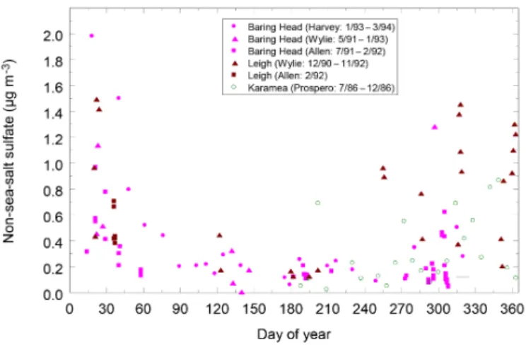
Figure 2.Non-sea-salt sulfate concentrations plotted against day of year at different New Zealand coastal atmospheric monitoring sites.
2002; Wylie and de Mora, 1996). Corresponding seasonality in nssSO4was observed, with a maximum (0.8–1.5 µg m−3)
in early austral summer at the start of the year, decreasing in late summer to 0.1–0.4 µg m−3through autumn and win-ter (see Fig. 2; Sievering et al., 2004; Allen et al., 1997). For comparison, coarse SSA dominates the aerosol mass at Bar-ing Head, with concentrations of 6–10 µg m−3(Jaeglé et al., 2011; Spada et al., 2015). Similar seasonal cycles of DMS and nssSO4were recorded at Cape Grim (Ayers, 1991), and
the observed diurnal inverse correlation between sulfur diox-ide and DMS at Baring Head was applied to estimate yield and the potential contribution to aerosols (de Bruyn et al., 2002). Consistent seasonal trends between activated parti-cles and cloud droplet number concentration were also appar-ent, with a summer maximum over the Southern Hemisphere (Boers et al., 1996, 1998), related to phytoplankton produc-tion (Thomas et al., 2010). Overall, the temporal trends in aerosol precursors and pathways do not follow that of wind speed and other physical drivers but instead reflect biological processes inferring control by surface ocean biogeochemistry (Korhonen et al., 2008).
3 Research programme and strategy
3.1 PreSOAP
A pilot study, PreSOAP, was carried out to test techni-cal approaches and confirm the regional source of biogenic aerosols in the Chatham Rise region on the New Zealand re-search vessel,Tangaroa, on 1–12 February 2011 (day of year, DoY, 32–42). The strategy of bloom location using satel-lite imagery and subsequent mapping of surface properties proved successful, with three blooms of differing DMSsw and pCO2 signatures located and monitored each for 3–
4 days. The first bloom was initially dominated by dinoflagel-lates with an increase in diatom biomass after 3 days, while the second and third blooms were primarily dominated by
coccolithophores and dinoflagellates, respectively. This vari-ability in species composition resulted in significant spa-tial and temporal variability in DMS concentrations in the MBL (DMSa) and DMSsw. DMSa concentration varied over 2 orders of magnitude, reaching 1000 ppt on DoY 36 (see Fig. 3b), similar in range to that recorded at the Baring Head station near Wellington (Harvey et al., 1993; de Bruyn et al., 2002). There was no significant correlation between DMS in the two phases, with DMSa showing a stronger relation-ship with wind speed (see Fig. 3). Surface Chla concentra-tions reached 2 mg m−3, but there was no significant relation-ship between DMSsw and Chla, with the DMSsw maximum of∼10 nmol L−1during the first bloom coinciding with an intermediate Chla of ∼1 mg m−3 (Fig. 3d). The observed temporal and spatial variability in DMSa and DMSsw dur-ing PreSOAP highlighted the technical challenge of estab-lishing relationships between surface ocean biogeochemistry and atmospheric composition. Provisional method develop-ment was also carried out for the measuredevelop-ment of DMS and other parameters in near-surface waters and the sea surface microlayer (SSM).
Surface DMSsw andpCO2were mapped, and DMSa and
CO2 MBL concentrations and fluxes were measured
con-tinuously by sensors and collectors mounted on the bow of the vessel. Testing of the eddy covariance (EC) flux tech-nique identified an issue with water vapor interference that dominated the CO2signal recorded by an open-path infrared
gas analyzer (IRGA). Preliminary studies also identified that residual ship motion dominated over turbulence for the real-time switching of relaxed eddy accumulation measurement of flux under high swell conditions. The logistical challenges of flux measurement at distance from the vessel were also assessed by deployment of a free-floating catamaran sup-porting a mounted gradient flux sampling system (Smith et al., 2017). A temperature microstructure profiler was also deployed to record near-surface temperature and turbulence structure (Stevens et al., 2005), although this was limited to short sampling periods, highlighting the need for a mounted thermistor array on a spar buoy for longer measurement cov-erage.
The utility of a baseline sector for sampling MBL com-position, using relative wind direction and speed, was also tested during PreSOAP. Measurements showed a tendency for higher condensation nuclei concentration in the “non-baseline” sector, confirming the utility of this approach (Har-vey et al., 2017). A common aerosol inlet provided clean air from a height of 17.5 m above sea level to instruments and sensors in a container laboratory on deck. Particle size dis-tribution and concentration, including ultrafine nuclei con-centrations, were continuously monitored using a scanning mobility particle sizer (SMPS) and optical particle counters (OPCs), with bulk ion chemistry samples collected using a high-volume sampler. The composition of primary marine aerosols was also examined using a 0.45 m3bubble chamber, in which sea spray was formed via the bursting of bubbles
Figure 3. Continuous measurements during PreSOAP of(a)wind speed (m s−1), (b) atmospheric DMS (ppt),(c)surface water DMS (nmol L−1)and(d)surface chlorophylla(mg m−3; quenched data removed).
produced by passing clean compressed air through sintered glass (Mallet et al., 2016).
3.2 The SOAP voyage
The SOAP voyage employed the strategy successfully pi-loted on PreSOAP of identifying phytoplankton blooms in NASA MODIS Aqua and Terra satellite ocean color im-ages with subsequent bloom location and mapping using a suite of underway sensors (Chl a,β660 backscatter,pCO2,
DMSsw). The blooms were discrete and coherent areas of elevated ocean color that were provisionally characterized by a concentration of 1 mg m−3 Chla or higher. For each bloom, a nominal center was identified, based upon maxi-mum DMSsw and Chlaconcentrations, and marked by de-ployment of a spar buoy. Repeat activities at the bloom cen-ter included the characcen-terization of the surface mixed layer by vertical profiling, the collection of SSM samples at a dis-tance from the main vessel and gradient flux on a catama-ran. Overnight mapping was carried out to determine changes in bloom magnitude and position. Sampling also took place at stations on the periphery and outside the blooms, as de-fined by distance from the bloom center and a clear demar-cation in surface biogeochemical variables. The SOAP voy-age was nominally divided into three different bloom periods (see Fig. 4), with an initial dinoflagellate bloom (B1) located 12 h into the SOAP voyage that exhibited elevated Chl a and DMSsw andpCO2drawdown, a coccolithophore bloom
(B2) with initially moderate signals that weakened, and a
fi-nal bloom (B3) of mixed community composition. Following a storm, the surface water column structure and biogeochem-istry were significantly different, and so this bloom was sub-divided into B3a and B3b.
3.2.1 Environmental conditions during the SOAP voyage
Back-trajectory analysis of particle density was calcu-lated for each bloom using the Lagrangian Numerical Atmospheric-dispersion Modelling Environment (NAME) for the lower atmosphere (see Fig. 5). The meteorological sit-uation evolved over the SOAP voyage from a high-pressure system with light winds during B1, to stronger winds during B2 and B3. The main weather features included a depres-sion crossing the central South Island on DoY 54–55 dur-ing B2 and a second depression from the east from DoY 58 onwards. During B3, a vigorous front advanced up the east coast of the South Island on DoY 61 with strong SW winds of 20 m s−1, followed by a depression crossing the lower North Island on DoY 63 that maintained a fresh southerly airflow for the remainder of the voyage. Air and water temperatures during B1were generally similar indicating near-neutral sta-bility, whereas B2 experienced a period of warm, moist air and reversal in direction of turbulent heat fluxes, followed by a short period when air temperatures were 2–3◦C higher on DoY 56–58 (See Fig. 6). Waves were dominated by swell from the south-southwest, with significant wave height mir-roring trends in wind speed, reaching a 5 m maximum
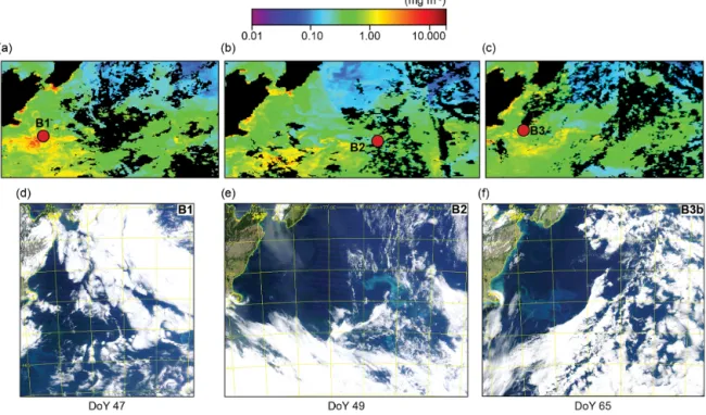
dur-Figure 4.Eight-day composite images of surface chlorophylla(MODIS, 4 km resolution) during the SOAP voyage for(a)10–17 Febru-ary 2012 (DoY 41–48),(b)18–25 February 2012 (DoY 49–56) and(c)26 February–4 March (DoY 57–64), showing bloom locations (red dots), with the color scale (mg m−3)above figures(a–c), and daily true-color images for(d)Bloom 1 (16 February 2012, DoY 47),(e)Bloom 2 (18 February 2012, DoY 49) and(f)Bloom 3 (3 March, DoY 65) (MODIS Aqua data courtesy of NASA).
ing the localized storm on DoY 61 (see Fig. 6). Wave pa-rameters obtained from NOAA WaveWatch III analyses in-dicated that wave height was 23 % lower during B1 and B3 and 13 % lower during B2, relative to wave height south of New Zealand at 50◦S.
Table 1 summarizes the hydrographic and biogeochemi-cal characteristics in the surface mixed layer of the three phytoplankton bloom regions. B1 was a large dinoflagellate bloom with high surface DMSsw (maximum∼30 nmol L−1; mean 16.8 nmol L−1; Bell et al., 2015) and Chl a (maxi-mum 3.4 mg m−3)and significant CO2undersaturation with
a mean surfacepCO2of 320 ppmv (see Table 1). B1 was
lo-cated south of the Mernoo bank, a deep channel between the western end of Chatham Rise and the east coast of the South Island. This region has been previously identified as a prime location for phytoplankton blooms, due to eddy-driven mix-ing and flow reversals arismix-ing from current and topographic interaction, which enhance iron and nutrient supply (Boyd et al., 2004). During B1, winds remained light (see Table 1) with a calm sea state, and the spar buoy drifted northeast primarily under the action of surface currents. Solar irradi-ance was high and a shallow surface mixed layer developed (see Fig. 6), with a significant near-surface temperature gra-dient (Walker et al., 2016). Mean nitrate and phosphate con-centrations (5.3 and 0.4 µmol L−1, respectively) were suffi-cient for phytoplankton growth, whereas silicate was low (see Table 1) and close to growth-limiting concentrations
(Boyd et al., 1999). Although dinoflagellates dominated, coc-colithophore biomass was higher at some stations, and na-noeukaryote abundance was generally low. B1 was occupied for 5–6 days, during which broader regional excursions with overnight mapping identified a bloom of high Chlabut rela-tively low DMSsw to the southwest.
The vessel relocated to a coccolithophore bloom, B2, ev-ident at the eastern end of the Chatham Rise in MODIS true-color satellite images (see Fig. 4b). Upon arrival on DoY 52, B2 showed an initial mean DMSsw of 9 nmol L−1 and elevated Chl a and was characterized by a relatively warmer, shallower, saltier surface mixed layer of lower ni-trate concentration (compared to B1; see Table 1), typical of subtropical water. This appeared to provide optimal condi-tions for coccolithophores as surface water backscatter (β660)
was initially elevated by high lith abundances, with coccol-ithophores accounting for up to 40 % of phytoplankton car-bon. However, the intrusion of warm, moist air associated with northwesterly winds, coincided with a reversal in the di-rection of turbulent heat fluxes and was followed by a south-west wind shift strengthening to 17 m s−1 by DoY 56 (see Fig. 6). This resulted in deepening and cooling of the sur-face mixed layer with a corresponding increase in nutrient concentrations, which, combined with a decrease in solar ir-radiance, resulted in a decline in Chlaand DMSsw (Bell et al., 2015).
T
able
1.
Summary
of
surf
ace
w
ater
characteristics
during
each
bloom
period.
All
v
alues
are
mean
±
1
standard
de
viation,
except
where
maximum
v
alues
are
also
sho
wn
by
<
.
*
indicates
v
alue
deri
v
ed
from
2
to
10
m
depth
on
all
stations
during
bloom
occupation;
#
indicates
continuous
m
easurement
in
surf
ace
w
aters
(nominal
6
m
depth).
Abbre
viations:
lat
–
latitude;
long.
–
longitude;
atmos.
press.
–
atmospheric
pressure;
irrad.
–
irradiance;
U
10
–
wind
speed
adjusted
to
10
m
height
(uncorrected
for
v
essel
flo
w
distortion);
H
s
–
significant
w
av
e
height;
MLD
–
mix
ed
layer
depth;
SST
–
sea
surf
ace
temperature;
Sal
–
surf
ace
salinity;
Chl
a
–
chloroph
yll
a
.
T
ime/Location
Meteorological
Hydrodynamic
Biogeochemical
Bloom
Start
NZST
(DoY
UTC)
End
NZST
(DoY
UTC)
Bloom
center
lat.
Bloom
center
long.
Atmos.
press.
mb
Irrad
W
m
−
2
U
10
Range
m
s−
1
H
s
m
MLD
m
*
SST
◦
C
#
Sal.
#
Nitrate/
phosphate/
silicate
µmol
L
−
1
*
Chl
a
mg
m
−
3
*
p
CO
2
ppmv
#
DMSsw
nmol
L
−
1
#
Dominant
ph
ytoplankton
*
B1
14/02/12,
02:00
(44.6)
19/02/12,
12:00
(50.0)
−
44.34
−
44.61
174.2
174.78
1019.1
±
2.9
232
<
1061
6.6
(5–
7.6)
2.0
14.5
±
1
14.5
±
0.4
34.48
5.3
±
0.9
0.43
±
0.2
0.35
±
0.1
0.84
±
0.2
<
3.4
320
±
24
16.8
±
1.5
Dinoflagellate
B2
21/02/12,
16:15
(52.2)
26/02/12,
12:00
(57.0)
−
43.55
−
43.71
180.16
180.32
1011.5
±
5.3
196
<
1079
10.4
(6.9–
12.4)
2.9
24.0
±
9
15.8
±
0.2
34.6
1.7
±
1.0
0.27
±
0.07
0.41
±
0.33
0.67
±
0.3
<
1.0
339
±
9
9.1
±
2.9
Coccolithophore
Dinoflagellate
B3a
27/02/12,
10:00
(57.9)
1/03/12,
04:00
(60.67)
−
44.11
−
44.61
174.47
174.88
1010.0
±
8.2
242
<
1212
10.3
(8.1–
12.1)
2.6
28.6
±
1.7
14.4
±
0.2
34.32
3.7
±
1
0.34
±
0.06
0.3
±
0.16
0.44
±
0.17
<
0.92
333
±
14
5.37
±
1.5
Mix
ed
B3b
02/03/12,
06:00
(61.7)
5/03/12,
17:00
(65.2)
−
44.19
−
44.78
174.3
174.93
1008.6
±
9.4
182
<
1016
12.6
(8.5–
14.9)
3.6
41.1
±
6
13.2
±
0.4
34.32
4.2
±
1.1
0.39
±
0.1
0.48
±
0.05
0.59
±
0.2
<
1.1
340
±
8
3.1
±
1.2
Mix
Figure 5. (a–c)Synoptic meteorology summary for each bloom period during the SOAP voyage. Surface pressure and wind plots (color scale to the left of panelsa–c) are derived from the New Zealand local area unified model NZLAM, with the bloom location indicated by a red dot.(d–f)Back-trajectory analyses for each bloom period during the SOAP voyage. This was calculated using the Lagrangian Numerical Atmospheric-dispersion Modelling Environment (NAME) for the lower atmosphere (0–100 m) as time-integrated particle density (g sm−3; color scale below figures). Each plot shows the back trajectory of eight “releases”, i.e., one every 3 h over 24 h for the actual ship position.
Following the 5-day occupation of B2, the vessel returned to south of Mernoo bank to assess a bloom that had devel-oped near the original site of B1. Surface biogeochemical signals were initially weak in B3a, with a mixed commu-nity of coccolithophores and dinoflagellates and low DMSsw (2.2 nmol L−1)and Chla(mean 0.39 mg m−3). However, an intense front advanced up the South Island and resulted in strong SW winds that exceeded 20 ms−1 (see Fig. 6), after
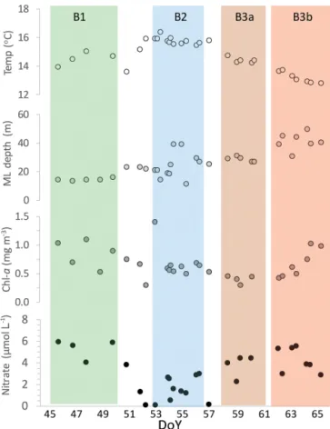
which mixed layer depth and associated nutrients increased. Consequently, stations before and after the storm were physi-cally and biogeochemiphysi-cally disparate. B3a stations exhibited similar sea surface temperature to B1, but with a deeper sur-face mixed layer and a Chlahalf that of B1, whereas B3b sta-tions were significantly cooler (at 13◦C) and deeper (41 m) than B1 (see Fig. 7), with higher silicate concentration due to enhanced vertical mixing. Subsequent stabilization of the surface mixed layer by light winds combined with elevated
nutrients stimulated Chla, diatom and coccolithophore abun-dance in the final B3b stations (see Figs. 6 and 7).
4 SOAP work programmes and observations
A number of parameters were measured (see Table 2) in three interlinked work programmes during the SOAP voyage, as indicated in Fig. 8 and detailed below.
4.1 The distribution and composition of aerosols, precursors and trace gases in the MBL
Aerosol number concentration, size distribution, compo-sition, water uptake and CCN concentration were mea-sured semicontinuously during SOAP to address the over-all paucity of aerosol observations and the apparent rarity of nucleation events over the remote ocean. These were
char-Table 2.Parameters sampled during the SOAP voyage. Key: C – continuous; D – discrete; W – workboat; *indicates instrument sampling on common aerosol inlet.
Measurement Mode Instrument
WP1 Atmospheric
Organic nuclei production C* Ultrafine organic tandem differential mobility analyzer (UFO-TDMA)
Aerosol water uptake and volatility C* Volatility humidity differential mobility analyzer (VH-TDMA)
Nucleation/Aitken mode size spectra C* Scanning mobility particle sizer (SMPS)
Condensation nuclei counts C* Condensation particle counter (CPC)
Accumulation mode aerosol number C Passive cavity aerosol spectrometer probe (PCASP)
Cloud condensation nuclei C* CCN spectrometer
Aerosol filter chemistry – major ions C Hi-vol, cascade, ion chromatograph
Black carbon C* Aetholometer
PM10aerosol filters C Organic functional groups by FTIR and inorganic composition
by ion beam analysis
Column aerosol D Sun photometer (Microtops II)
Nascent sea spray composition via bubble burst of seawater samples
D Chamber experiments
DMS C MesoCIMS (chemical ionization mass spectrometry)
CO2and methane C Picarro CRDS
Halocarbons, iodine and halogen oxides C µ-Dirac electron capture detector–gas chromatograph and multi-axis differential optical absorption spectroscopy (Max-DOAS)
VOCs (acetone, DMS, acetonitrile, methanol, methanethiol, isoprene, monoterpenes, acetaldehyde)
C Proton transfer reaction mass spectrometer (PTR-MS)
VOCs C5to C15 D Pre-concentration and TD-GC-FID/MS
Aldehydes, ketones (incl. dicarbonyls), C2to C8 D Derivatization and HPLC
WP2 physics
DMS flux C MesoCIMS (chemical ionization mass spectrometry)
CO2EC flux C LI-COR infrared gas analyser (IRGA), sonic anemometer
mo-tion sensors
DMS gradient flux D Catamaran, SCD-GC
Near-surface T and S D Conductivity–temperature–depth (CTD)
Near-surface stratification C Spar buoy – temperature array, microcats
Near-surface turbulence C Vector, FastCat
Sea state C NOAA Wavewatch III
Whitecap coverage D Campbell Scientific 5-megapixel Camera
Meteorological conditions C Automatic weather station (AWS)
Bulk fluxes C Eppley radiometers, rain gage; Eppley Precision Spectral
Pyranometer (PSP)
MBL height and stability D Radiosonde
WP3 ocean biogeochemistry
Chlorophylla C, D, W Ecotriplet
Backscatter andβ660backscatter C Ecotriplet
pCO2 C IRGA
pH C, D, W Spectrophotometer
Dissolved inorganic carbon (DIC) D
Nutrients D, W Colorimetric autoanalyzer
Dissolved organic carbon (DOC) D, W High-temperature catalytic oxidation (HTCO)
CDOM D, W Spectrophotometer
Particulate organic and total carbon and nitrogen and isotopes (POC/PON/PC/PN/13C/15N)
D Mass spectrometer
Fatty acids and alkanes D, W
Dissolved DMS C, MiniCIMS (chemical ionization mass spectrometry)
Dissolved DMS D, W SCD/FPD (flame photometric detector)
DMSP and processes D, W SCD
Pigments D HPLC
Microbial community abundance D, W Flow cytometry
Phytoplankton identification/counts D, W Optical microscopy
Figure 6.Meteorological and hydrodynamic variables during the SOAP voyage, including(a)wind speed (W.s., ms−1);(b)direction (Dir., ◦); wind (blue) and wave (cyan);(c)temperature (Temp.,◦C); air (black) and surface water (green);(d)irradiance (Irrad., W m−2)and
(e)significant wave height (Hs, m). Bloom occupation periods are indicated by the red horizontal bars and bloom labels in the upper panel.
acterized by a suite of instruments covering a particle size range of 0.01 to 10 µm (see Fig. 9 and Table 2), which enabled the determination of the size-dependent contribu-tion of PMA and nssSO4 to aerosol and CCN
concentra-tions. Aerosol characterization identified variable Aitken and consistent submicron-sized accumulation and coarse modes, with the submicron aerosol mass dominated by secondary aerosol with ammonium sulfate/bisulfate under light winds and with an increase in sea salt proportion as local winds increased. Ongoing data analysis is examining whether sig-nificant nucleation events occurred.
The operational mode for underway aerosol measurement was to slowly steam at 1–2 kn into the prevailing wind, across an area of high biological productivity or a signifi-cant air–sea gas gradient, generally between noon and 14:00 when solar irradiance was maximal. The common aerosol in-let developed during PreSOAP allowed uncontaminated air from above the bridge to be sampled when the wind was on the bow, thus minimizing interference from ship stack emissions. Contamination events were screened out using a real-time clean-sector sampling “baseline” flag and switch (Harvey et al., 2017), enabling the clean collection of in-tegrated samples. Although the vessel exhaust was the pri-mary contaminant, other potential sources included the
work-boat and recirculation of polluted air around the ship, and longer-range terrestrial influences were also assessed. Mea-surements of black carbon using an aethalometer and CO2by
high-precision cavity ring-down laser spectroscopy (CRDS) provided two independent variables for detecting contami-nation events, and some VOCs, measured by proton trans-fer reaction mass spectrometer (PTR-MS; see Table 2), were also used as indicators of diesel combustion. The vessel was orientated into the wind as often as possible, which resulted in a high frequency (∼75 %) of baseline sector conditions during the SOAP voyage. Clean marine air periods were defined post-voyage, using the baseline wind sector (225– 135◦relative to bow and wind speed greater than 3 m s−1), black carbon concentrations (less than 50 ng m−3)and back trajectories, and indicated minimal terrestrial impact (peri-ods when the minimum number of hours over land in 72 h back trajectory is zero), with periods of workboat opera-tions removed. An ensemble of Hybrid Single-Particle La-grangian Integrated Trajectory (HYSPLIT) model back tra-jectories (Draxler and Rolph, 2013) was run for each hour of the voyage, and NAME back trajectories were calculated for every 3 h (Fig. 5; Jones et al., 2007). Figure 10 shows particle number and CCN concentrations compared to the number of hours the 72 h back trajectory spent over land
cal-Figure 7.Surface water properties (2–10 m) recorded at each sta-tion during the SOAP voyage: temperature (Temp,◦C), mixed layer depth (ML depth, m), chlorophylla (Chl-a, mg m−3)and nitrate concentration (µmol L−1)plotted against day of year (DoY), with the occupation period for each bloom indicated by the vertical shaded bars and bloom labels at the top of the figure.
culated from HYSPLIT trajectories. Particle concentrations were generally higher during periods of terrestrial influence (see DoY 52 and 60; Fig. 10), with average particle number concentrations of 1122±1482 cm−3, double that observed for clean marine air. Ion beam analysis also revealed the pres-ence of silicate and aluminium on ambient submicron filter samples, suggesting a terrestrial source and supporting the back-trajectory modeling of continental outflow.
During the initial occupation of B1 under light winds, the particulate matter (PM10) total ion mass was 9.5 µg m−3
compared to subsequent samples under higher winds in the range 20–50 µg m−3. The dominant components of the
inor-ganic mass fraction were sea salt ions and nssSO4, although
a measurable organic fraction was also present (see below). The NaCl mass in light winds during B1 was 6.6 µg m−3with >95 % being>3 µm in diameter, relative to 32.5 µg m−3 un-der stronger winds during B3b. Although 72 % was>3 µm, the largest difference in mass occurred in the 1.5 to 3 µm size range. In contrast, the mass of nssSO4 was predominantly
submicron sized; B1 exhibited the largest nssSO4 mass at
2.0 µg m−3with 85 % in sizes<1 µm, whereas in B3b, the nssSO4mass was much lower at 0.6 µg m−3with 76 % with
sizes <1 µm. These results confirm the influence of both physical and biogeochemical processes on aerosol compo-sition.
Voyage particle number concentrations during clean ma-rine periods averaged 534±338 cm−3, with CCN concen-trations of 178±87 cm−3 (±1 sd) at 0.5 % supersatura-tion and an average particle fracsupersatura-tion activated into CCN of 0.4±0.2. Bloom average particle number concentrations ranged from a minimum of 385±96 cm−3in B3b to a max-imum 830±255 cm−3at the start of B2 (Fig. 10). B1 dis-played the highest CCN activation ratio, of 0.5±0.2, po-tentially due to the combination of low wind speeds, large biogeochemical signals and SMA fluxes. Comparison of the inorganic ion mass, determined from high-volume sampler filters, between the different blooms does not support the conclusion that the B1 activation ratio was higher simply because particles were larger. As the median particle di-ameters during clean marine periods were consistent be-tween the three blooms, this suggests that particle com-position, secondary organics or coagulation may have im-pacted CCN activation at B1. These findings are supported by preliminary results from an application of the ACCESS-UKCA model (M. Woodhouse, personal communication, 2017), which simulated the additional impact of emissions of marine secondary organic carbon under the conditions de-termined during SOAP. In contrast, the average CCN acti-vation ratio for B3a was lower at 0.13±0.06. Nucleation mode particles (10 and 15 nm) were measured by ultrafine organic tandem differential mobility analyzer (UFO-TDMA; Vaattovaara et al., 2005) and Aitken mode particles (50 nm) by UFO-TDMA and a volatility and hygroscopicity tandem differential mobility analyzer (VH-TDMA; Johnson et al., 2004; Villani et al., 2008). This analysis typically identi-fied a significant (up to 50 % volume fraction) secondary organic component during sunny conditions in bloom re-gions, particularly during B1. The TDMA results provided further evidence for secondary organic aerosol processing of the dominant secondary nssSO4mode during B1.
Deliques-cence measurements (VH-TDMA) indicate that the Aitken mode population is largely comprised of neutralized nssSO4,
i.e., ammonium sulfate. Small and sporadic contributions to the Aitken mode from a nonhygroscopic component (num-ber fraction up to 0.4) and a highly hygroscopic component (number fraction up to 0.3) were observed in addition to the secondary nssSO4mode (number fraction of 0.6–1). The
wa-ter uptake and volatility of the sporadic highly hygroscopic mode indicates that this may be composed of PMA.
The in situ aerosol size, number and composition measure-ments in the MBL were complemented by in vitro chamber measurements of nascent SSA to determine the PMA organic volume fraction and water uptake properties. Nascent SSA filter samples were analyzed using Fourier transform infrared spectroscopy (FTIR) for organic functional groups (Russell
Figure 8.Conceptual figure of the parameters, processes and vertical range measured during SOAP, with the integrated work programmes (WP) indicated on the left of the figure. CN: condensation nuclei. NSS: non sea salt.
Coarse mode Accumulation
mode Aitken
mode Nucleation
PCASP Hi-vol
SMPS
VH-TDMA (volatility-humidity) CCN (0.5 %)
Grimm
UFO-TDMA (ultrafine organic)
0.01 0.1 1 10
Diameter (µm)
CPC 3772/3007/3010
Figure 9. Aerosol characterization during SOAP, indicating size spectral (red) and total count (black) range for each instrument, rel-ative to aerosol size and mode. Ambient RH measurement was used for RH correction of the PCASP, Hi Vol and SMPS, and diffusion driers (Silica Gel) were used on the inlet of the UFO-TDMA and VH-TDMA.
et al., 2011) and ion beam analysis for inorganic concentra-tions (Cohen et al., 2004). Measurements of the hygroscopic growth factor and the volatile fraction up to 450◦C for 50– 150 nm particles using the VH-TDMA were compared with those of reference inorganic samples (e.g., sea salt, ammo-nium sulfate) to determine their organic volume fractions (Modini et al., 2010). Complementing the VH-TDMA, the UFO-TDMA provided further information on the organic
content of particles of 50 nm and down to 10 nm. The bub-ble chamber observations indicated that the PMA contained a substantial primary organic fraction. VH-TDMA results in-dicate that the Aitken mode PMA was primarily nonvolatile (78–93 %), with an average organic volume fraction of 51 % (ranging from 39 to 68 %), and the UFO-TDMA results show an organic volume fraction (OVF) ranging from 35 to 45 %. These results are consistent with observations in the North Pacific and Atlantic, for which an Aitken mode volatile frac-tion of the order of 15 % and OVF of 0.4–0.8 have been ob-served (Quinn et al., 2014). FTIR analysis indicated that the POA aerosol in the chamber experiments was largely com-posed of hydroxyl functional groups, with minor contribu-tions from alkanes, amines and carboxylic acid groups, con-sistent with previous observations (Russell et al., 2011).
Although DMS was a primary focus of measurements dur-ing SOAP, a wide variety of other VOCs that potentially contribute to secondary organic aerosol formation were also measured. Halogens and halogen oxides were measured us-ing multi-axis differential optical absorption spectroscopy (Max-DOAS) and electron capture detector–gas chromatog-raphy (ECD-GC). Iodine has been identified as a poten-tially important precursor of nucleation in coastal regions (Sellegri et al., 2005), and SOAP provided an opportunity to relate the presence of halogen oxides to phytoplankton biomass and composition in the surface ocean and nucle-ation events in the MBL. A high-sensitivity PTR-MS carried out measurements continuously in H3O+mode in the range